of their algorithm was later published by Berger and ... dimensional Berger-Colella AMR hierarchy is an ..... [10] Michael L. Norman, John M. Shalf, Stuart.
High-quality Volume Rendering of Adaptive Mesh Refinement Data Gunther H. Weber1,2,3 , Oliver Kreylos1,3 , Terry J. Ligocki3 , John M. Shalf 3,4 Hans Hagen2 , Bernd Hamann1,3 , Kenneth I. Joy1 and Kwan-Liu Ma1
2
1 CIPIC, Department of Computer Science, University of California, Davis, USA AG Computergraphik, Department of Computer Science, University of Kaiserslautern, Germany 3 NERSC, Lawrence Berkeley National Laboratory, Berkeley, USA 4 NCSA, University of Illinois, Urbana-Champaign, USA
Abstract Adaptive mesh refinement (AMR) is a numerical simulation technique used in computational fluid dynamics (CFD). By using a set of nested grids of different resolutions, AMR combines the simplicity of structured rectilinear grids with the ability to adapt to local changes in complexity in the domain. Without proper interpolation on the boundaries of grids of different levels of a hierarchy, discontinuities can arise. Treating locations of data values given at cell centers of AMR grids as vertices of a dual grid creates gaps between hierarchy levels. Using an index-based tessellation approach that fills these gaps with “stitch cells” we define an interpolation scheme that avoids discontinuities at level boundaries. We use the resulting interpolation scheme to generate volume-rendered images. Modifying transfer functions on a per-level basis allows us to emphasize (or de-emphasize) a specific level and gain a better understanding of the underlying hierarchical structure.
1
Introduction
AMR was introduced to computational physics by Berger and Oliger [2] in 1984. A modified version of their algorithm was later published by Berger and Colella [1]. AMR has become increasingly popular especially in the computational physics community. Today, it is used in a variety of applications. For example, Bryan [3] has used the technique to simulate astrophysical phenomena using a hybrid approach of AMR and particle simulations. Figure 1 shows a simple two-dimensional (2D) AMR hierarchy produced by the Berger–Colella method. The basic building block of a d– VMV 2001
Figure 1: AMR hierarchy consisting of four grids in three levels. Grid boundaries are drawn as bold lines. Locations at which dependent variables are given are indicated by solid discs. dimensional Berger-Colella AMR hierarchy is an axis-aligned, structured rectilinear grid. Each grid g consists of hexahedral cells and is positioned by specifying its local origin og . AMR typically uses a cell-centered data format, i.e., dependent function values are associated with cell centers. Since location and connectivity can be inferred from the regular grid structure, it suffices to store dependent data values in arrays. An AMR hierarchy consists of several levels Λl comprising one or multiple grids. All grids in the same level have the same cell size. A hierarchy’s root level Λ0 is the coarsest level. Each level Λl may be refined by a finer level Λl+1 . A grid of a refined level is referred to as a coarse grid and a grid of a refining level as a fine grid. A refinement ratio r specifies how many fine grid cells fit into a coarse grid cell, considering all axial directions. Stuttgart, Germany, November 21–23, 2001
data sets. To avoid discontinuities and re-sampling problems they introduce an approach based on dual grids: By interpreting the locations of cell-centered data values as vertices of a new dual grid they avoid the need for re-sampling. The use of a dual grids produces gaps between hierarchy levels. Using a scheme related to that used by Gross et al. [5], Weber et al. fill these gaps via a generic stitching scheme using deformed hexahedra, triangular prisms, pyramids and tetrahedra. Direct volume rendering is, besides the extraction of isosurfaces and slice-based methods, the most common visualization method for scalar volume data. Using so-called transfer functions, scalar values are “mapped” to illumination and color properties. Regions in the volume are associated with color/illumination properties that a transfer function assigns to scalar values. Direct volume rendering methods can be differentiated by their underlying illumination models (i.e., by the “optical properties” of transfer functions) and whether they operate in image space or object space. Image-space-based algorithms, e.g., ray casting [11], operate on pixels in screen space as “computational units,” i.e., they perform computations on a per-pixel basis. Objectspace-based methods, like cell-projection [7], operate on cells as computational units, i.e., they perform computations on a per-cell basis. Max [9] surveys various optical models used for volume rendering. Weber et al. [12] present two volume rendering schemes for AMR data. One scheme is a hardware-accelerated renderer for previewing, the other scheme is based on cell projection and allows the progressive rendering of AMR hierarchies. It is possible to render an AMR hierarchy starting with a coarse representation and refining it by subsequently integrating the results from rendering finer grids.
This value is always a positive integer. A refining grid refines an entire level Λl , i.e., it is completely contained in the region covered by that level but not necessarily in the region covered by a single grid of that level. Each refining grid can only refine complete grid cells of the parent level, i.e., it must start and end at the boundaries of grid cells of the parent level. The Berger-Colella scheme [1] requires a layer with a width of at least one grid cell between a refining grid and the boundary of the refined level. We generate volume-rendered images from AMR data using a cell-projection approach. For interpolation purposes, dependent data values should be associated with a cell’s vertices rather than its center. To avoid a re-sampling step, we interpret the locations of the samples as vertices of a new grid and use this dual grid for interpolation. The use of dual grids creates gaps between grids of different hierarchy level. We fill those gaps in an index-based stitching step. The resulting stitch mesh can be used to define an interpolation scheme for the whole domain of a data set. We use this interpolation scheme for progressive volume rendering of AMR hierarchies, i.e., we start with an image obtained by rendering a coarse level and refine this image by incorporating the results produced by rendering finer levels. In addition, we introduce a method that allows a user to emphasize or de-emphasize certain levels by modifying the transfer functions used for volume rendering on a per-level basis. For each level, an opacity weight and a saturation weight are specified. A base transfer function is multiplied with these weights to obtain a level transfer function.
2
Related Work
Little research has been done to date regarding the visualization of AMR data. Published work has mainly focused on converting AMR data into suitable conventional representations and visualizing these, see Norman et al. [10], while preserving the original hierarchical structure as much as possible. Ma [6] describes a parallel rendering approach for AMR data. Even though he re-samples the data to vertex-centered data, he still uses the hierarchy and contrasts this approach to re-sampling the data to the finest available resolution. Max [8] describes a sorting scheme for cells for volume rendering and uses AMR data as one application of his method. Weber et al. [13] extract isosurfaces from AMR
3
Dual Grids and Grid Stitching
Most interpolation techniques expect dependent data values to be located at a cell’s vertices, while grids in an AMR hierarchy typically use a cellcentered format. By using the dual grid, i.e., the grid defined by the locations of the function values at the cell centers, it is possible to avoid a resampling step and use the original data values for interpolation purposes. 122
y v’1 (z)
v3
v0
x v’3 (z)
v4
z
v1
y v3
v’0 (y)
1
z
v1
v2
v’1 (x)
y
Figure 2 shows the dual grids for the first two levels of the AMR hierarchy shown in Figure 1. We note that the dual grids have “shrunk” by one cell in each axial direction when compared to the original grid. The result is a gap between the coarse grid and the embedded fine grids. In order to interpolate values in these gaps, we use a tessellation scheme that “stitches” grids of two different hierarchy levels. The resulting stitch mesh is constrained by the boundaries of the coarse and the fine grids and can be used to merge levels seamlessly. This stitch mesh must not subdivide any boundary elements of the existing grids, only existing faces, edges and vertices can be used and may not be subdivided. In Weber et al. [13], an index-based scheme is used to generate stitch cells. Boundary faces, edges and vertices of a fine grid must be connected to a coarse level. In the simple case of a single fine grid that is embedded in a coarse grid, the rectangles comprising a fine-grid boundary face must be connected to a coarse-grid vertex, edge or rectangle. The cell types resulting from these connections are pyramids, deformed triangle prisms and deformed hexahedral cells. A fine-grid edge must either be connected to two perpendicular edges (resulting in two tetrahedral cells) or two quadrilaterals (resulting in two deformed triangular prism cells) of the coarse grid. Each fine-grid vertex is connected to three quadrilaterals of the coarse grid via pyramid cells. When a coarse grid is refined by more than one fine grid, each coarse-grid point must be checked
x
(ii) Standard triangular prism
v4
v’1 (y)
v’0 (x)
p v3
1
v5
(i) Unit cube
Figure 2: Dual grids of the three AMR grids comprising the first two hierarchy levels shown in Figure 1. The original AMR grids are drawn in dashed lines and the dual grids in solid lines.
v5
v6 p
v0
v’0 (z) 1
v’3 (x)
v4 v’2 (z)
v7
z
y
v2
v1
v’3 (y)
p v0
v3 v2
p x
v0 1
v’2 (y)
(iii) Standard pyramid
z
v2
x
v1
(iv) Standard tetrahedron
Figure 3: Base elements for interpolation. for refinement. If a fine-grid boundary edge is adjacent to a boundary edge of another fine grid, this edge must be “upgraded” to the quadrilateral case by connecting it to the adjacent edge. Vertices can be upgraded to edges, or even quadrilaterals when several grids meet at a given location. All possible refinement configurations of coarse-grid points result in a large number of possible cases that needs to be considered when a fine grid is connected to a coarse level. Weber et al. [13] describe in detail how to deal with these cases.
4
Interpolation
We use the standard elements shown in Figure 3 for interpolation by mapping all cells generated in the stitching process to the appropriate standard element. All cells generated in our stitching approach have either triangular or quadrilateral faces. On boundary faces we have to ensure that interpolation yields consistent results, regardless of element type. We use bilinear interpolation for quadrilateral faces and linear interpolation (based on the barycentric coordinates of the interpolated point) for triangular boundary faces. 123
s out
Scan conversion tin
Front−facing part Single grid cell
s in
s out
t out t t in
1 p s in
Ray−segment queues Screen
Screen
Figure 4: Cell projection.
1
x
Figure 5: The transformation between a stitch cell and its standard element is linear. Line ray segments in the stitch cell are mapped to line segments in the standard element.
Values in the unit cube 3(i) are interpolated using standard trilinear interpolation which corresponds to bilinear interpolation when restricted to the boundary faces. In the case of a triangular prism cell, see Figure 3(ii), we first compute the values at the vertices of the triangle containing the point p (i.e., the triangle that is obtained by intersecting the prism with a plane being parallel to its two triangular end faces and containing p) by linear interpolation in x–direction. The value at p is obtained by linear interpolation within this triangle. Interpolation in pyramid cells, see Figure 3(iii), is done by a combination of bilinear and linear interpolation. To obtain a function value for a point p, we first interpolate linearly along the four side edges emanating from the point (0, 1, 0): This step interpolates the values at the vertices of a square in the y = constant plane containing p. Subsequently we interpolate bilinearly in the y = constant plane. Linear interpolation is used for tetrahedral cells. p is expressed in term of its barycentric coordinates and these are used as interpolation weights.
5
y
t
t out
t
cing par
Back−fa
and a back-facing part (faces with normals directed away from the viewer). First, the front-facing part is scan-converted into a buffer. For each pixel influenced by a cell, this buffer holds a depth corresponding to an entry parameter, called tin , along the ray and an interpolated scalar value at that position. Subsequently, the back-facing part is scanconverted. For each generated pixel, the depth corresponding to the exit parameter, called tout , along the ray and an interpolated scalar value are computed. The entry parameter value tin and the corresponding scalar value are read from the buffer, and the ray segment from tin to tout is constructed. This ray segment is inserted into the ray-segment queue of the corresponding pixel. If the ray segment is adjacent to existing ray segments in the ray-segment queue, it is merged with them. Two ray segments are adjacent when the union of their parameter intervals along the ray, given by the intervals ([t0,in , t0,out ] and [t1,in , t1,out ]) is “continuous,” i.e., when either t0,in = t1,out or t0,out = t1,in holds. When all cells are processed, each ray segment buffer contains only one ray segment corresponding to the complete ray originating from the pixel. To create ray segments, interpolated values must be computed along these segments. As mentioned in Section 4, this is done by mapping each cell to its corresponding standard/unit element and using the interpolation function for that element. Mapping a cell to its associated standard element can be integrated into cell projection. For each vertex, we store its physical coordinates and corresponding coordinates in its standard element. When cell faces are scan-converted using physical coordinates, the standard-element coordinates are linearly interpolated on the face and stored along with depth val-
Cell Projection
Cell projection [7] is an object-space-based method for volume rendering. It is similar to ray casting, a widely used image-space approach. Both methods trace rays through the volume, accumulating light along each ray. Ray casting does this on a perpixel basis. Cell projection methods construct ray segments passing through the individual cells and merge them. We maintain a priority queue for each pixel that collects all ray segments contributing to that pixel. Figure 4 shows the fundamental idea of our implementation of cell projection. Boundary faces of cells are divided into two parts, a front-facing part (faces with normals directed toward the viewer) 124
ues. Thus, points sin and sout are known for a ray segment in standard-element space along with its entry and exit parameter values tin and tout . All cells generated by our stitching approach, and the specific AMR meshes that we are dealing with, can be mapped to standard elements by a linear mapping: Line segments within a cell are mapped to line segments within a standard element. Thus, it is possible to obtain values along a ray segment by linearly interpolating the position in the standard element between sin and sout and using the standardelement interpolation function for this position, see Figure 5. We use the absorption and emission light model described by Max [9]. We specify emission by three components (red, green and blue) and absorption by one achromatic component, which implies that this component has the same effect on all color components. During cell projection, we compute transparency and emission for parts of ray segments that intersect a cell. The transparency function for a cell is given by �s (1) TC (s) = exp − τ (x)dx ,
layer of material of unit thickness having an extinction coefficient τ (s).) We define this opacity value α(s) as � � α(s) = 1 − exp −τ (s) , (5) If we approximate the integrals in Equations 1 and 2 numerically by the Riemann sum using equidistant samples si with a constant spacing ∆x between consecutive samples we obtain approximations for a cell’s transparency TC,approx (s) =
EC,approx (s) = n i=0
with
6 (2)
i−1 ��
�∆x 1 − α(si ) , (7)
j=0
�∆x o(si ) = 1 − 1 − α(si )
(8)
Progressive Cell Projection of AMR Data
We render an AMR hierarchy by subsequently cellprojecting its constituent levels. Two schemes are possible: Bottom-up rendering which first renders the finer levels and proceeds with filling gaps by rendering the corresponding portions of the coarser levels. In a top-down approach, a coarse level is rendered first. The result can be displayed and used as an intermediate visualization. An image is refined by proceeding to the finer levels and replacing portions of an already rendered image with versions at higher resolution. A bottom-up rendering scheme starts with cellprojecting the grids of the finest level. Grids of the coarser levels are cell-projected subsequently. While rendering coarser grids, cells overlapped by a finer grid must be skipped. Ray segments for the regions covered by these cells are already computed using a representation at a higher resolution. This is
The two values TC and EC are stored for each ray segment. Two adjacent ray segments S1 and S2 with transparencies TS1 and TS2 and emission contributions ES1 and ES2 , respectively, are merged into a larger segment with combined transparency (3)
and combined emission ,
C(si )o(si )
This is equivalent to compositing the samples, see [14]. To approximate ray segments within a cell, we use Equations 6 and 7 with a fixed number of samples (usually two samples per cell).
tin
Ecombined = ES1 + TS1 ES2
(6)
and emission contribution
where τ (x) denotes the extinction coefficient. The transparency of a cell is computed as TC = TC (tmax ), and its emission contribution as
Tcombined = TS1 TS2
�∆x 1 − α(si )
i=0
tin
tout � EC = C(s)τ (s)TC (s)ds.
n � �
(4)
where we assume that S1 is the ray segment closer to the screen. Instead of specifying the extinction coefficient τ in the transfer function, we specify and use an opacity value α(s). (Opacity specifies the percentage of light that remains after a ray has passed through a 125
ginning of the first level (p1 ), one that is contained within the first level (from p1 to p2 ) and one after the exit point from the first level (from p2 to p3 ). The region from v to p0 is “empty” and contains no cells. No ray segments are created for this region. Using an approach of partitioning rays into segments that are affected by finer grids and those that are not, it is straightforward to refine an already rendered image by rendering a finer level. Before a finer level is rendered, all ray segments affected by the finer level are erased from the ray-segment queues. When the level grid is rendered, the gaps in the ray segments resulting from this step are filled with more accurate ray segments, resulting in an overall improved image.
L0
p3
L1
p2
L2
p1
p0 v
Figure 6: Progressive rendering of AMR hierarchy.
7
done by using an intersection map. The intersection map contains an entry for each cell of the original AMR grid that specifies the index of the grid that overlaps it, should such a grid exist. In Weber et al. [12], the original grid is used to calculate interpolated values. Thus, for each cell, there exits a unique finer grid that refines it. Each cell of the dual grid used in our current approach is defined by eight vertices. Each of these vertices corresponds to a cell of the original AMR grid and can be refined by a different grid. It is no longer possible to specify a single grid that refines a given cell. However, it is still possible to specify, for each cell, whether it is refined by finer levels. If at least one of the original AMR cells corresponding to one of the vertices of a cell is refined, then that cell must be skipped. Unfortunately, this prevents us from performing refinement on the basis of single AMR grids. In our new approach, we must use complete levels when generating a refined image.
Level-dependent tions
Transfer
Func-
When rendering a hierarchical data set it is often desirable to emphasize or de-emphasize certain levels. For example, it is possible that a coarser level is used to specify only the “context” within which a finer level resides, but otherwise this coarser level might be of little interest. In this case, the coarse level should not hide relevant information present in the finer level. One way to achieve this is to deemphasize the coarse level and render it with lower opacity, i.e., to scale the opacity portion of the transfer function by a level-specific constant. By specifying a constant for each level, and modifying the transfer function for that level accordingly, it is possible to specify how much a level influences the final image. Another possibility to de-emphasize a level is to scale its color saturation. This can be done by converting RGB color values from the transfer function into HLS or HSV color space and scale the saturation by a second, level-dependent color map. Decreasing the saturation of a level does not prevent it from hiding details of a finer level, but this method adds the possibility to distinguish levels and illustrate their presence in a final image.
The top-down approach is modified in a similar way. The supplemental information added to each ray segment specifies the level in which a segment was created and the level that affects it (either the next finer level or no level) rather than specifying grid indices. Ray segments are merged only when they are adjacent, were created in the same level and are affected by the same level. Figure 6 shows a ray traced from a specific viewpoint. After rendering the root level L0 , the ray-segment queue corresponding to this ray contains three ray segments: one spanning from the entry point in p0 to the be-
8
Results
Figures 7 and 8 show results from rendering the “bubble” data set. This data set is the result from a simulation of a shock wave passing through an 126
cell between a refining grid and the boundary of a refined level. Even though Bryan [3] abandons this requirement, we still require it to be satisfied. This is necessary, because this requirement ensures that only transitions between a coarse level and the next finer level occur in an AMR hierarchy. Allowing transitions between arbitrary levels would result in the need to consider too many cases during the stitching process. (The number of cases would be limited only by the number of levels in an AMR hierarchy, since within this hierarchy transitions between arbitrary levels are possible.) These requirements are equivalent to the requirements described in [5] that also prevent transitions between arbitrary levels. Unfortunately, this requirement prevents us from handling the full range of AMR data sets generated, e.g., those produced by the methods of Bryan [3]. To handle the full range of AMR grid structures, our whole grid-stitching approach must be extended. Any lookup-table approach has inherent problems since the number of possible level transitions is bounded only by the number of levels in the hierarchy. The generation of ray segments during cell projection can be improved as well. More advanced lighting models and numerical integration schemes can be used. Furthermore, alternative interpolation functions for pyramid cells could be explored. We also plan to support refinement on a per-grid basis instead of a per-level basis. Our cell projection scheme is completely implemented in software and does not utilize special purpose graphics hardware. Even though this results in longer computation time this fact will allow us to parallelize our approach.
Argon–bubble surrounded by another gas. The visualized scalar field is gas density. The simulation result is stored in AMR format with a 80 × 32 × 32 root-grid resolution. In the initial time step, this grid is refined by 204 grids in a three-level hierarchy. Rendering all levels of the initial time step takes about two minutes and 23 seconds. Figures 7(ii), 7(iii) and 7(iv) show the results from rendering one time step near the end of the simulation. This time step consists of three hierarchy levels containing 682 grids in total. Rendering the root level required approximately 57 seconds, rendering the first level one minute and 42 seconds and rendering the second level three minutes and 41 seconds. The improvement in image quality by using the finer levels is clearly visible. Figure 8 shows another time step form the same data set. Rendering time was 40 seconds for the root level, one minute and 32 seconds for the first level and two minutes and 48 seconds for the second level. This time step consisted of 525 grids in total. Rendering times were one minute and 23 seconds for the root level, one minute and 55 seconds for the first level and four minutes for the second level. The quality improvement from using finer representations is clearly visible. (All time measurements were done on a 700 MHz Pentium III processor and using a Linux system.) Figure 9 show images generated from an astrophysical simulation of a star cluster. Figures 9(i), 9(ii) and 9(iii) show images resulting from rendering one, two and three levels. Here, the quality improvement is not so obvious, because features of the coarse root level hide details from the finer levels. In Figure 9(iii), the opacity of the root level is scaled by a factor of 0.6 and the opacity of the first level by a factor of 0.8. Details of the finer level are clearly visible while retaining features from the coarse levels as orientation aid. In Figure 9(iv), the saturations of root and first level are scaled by a factor of 0.2 in addition to the opacity weights. This further de-emphasizes these levels and allows us to clearly distinguish between the details in the third level and the “context” provided by the first two levels.
9
10
Acknowledgments
This work was supported by the Directory, Office of Science, Office of Basic Energy Sciences, of the U.S. Department of Energy under Contract No. DE-AC03-76SF00098; the Lawrence Berkeley National Laboratory; the National Science Foundation under contracts ACI 9624034 and ACI 9983641 (CAREER Awards), through the Large Scientific and Software Data Set Visualization (LSSDSV) program under contract ACI 9982251, and through the National Partnership for Advanced Computational Infrastructure (NPACI); the Office of Naval Research under contract N00014-97-1-0222; the Army Research Office under contract ARO 36598-MA-RIP; the NASA Ames Research Center through an NRA award under contract NAG2-1216; the Lawrence Livermore National Laboratory under ASCI ASAP Level2 Memorandum Agreement B347878 and under Memorandum Agreement B503159; and the North Atlantic Treaty Organization (NATO) under contract CRG.971628 awarded to the University of California, Davis. We also acknowledge the support of ALSTOM Schilling Robotics and SGI. We thank the members of the NERSC/LBNL Visualization Group; the LBNL Applied Numerical Algorithms Group; the Visualization and Graphics Research Group at the Center for Image Processing and Integrated Computing (CIPIC) at the University of California, Davis, and the AG Graphische Datenverarbeitung und Computergeometrie at the University of Kaiserslautern, Germany.
Future Work
Several extensions to our approach are possible. The original AMR scheme by Berger and Colella [1] requires a layer with a width of at least one grid 127
References [1] Marsha Berger and Phillip Colella. Local adaptive mesh refinement for shock hydrodynamics. Journal of Computational Physics, 82:64–84, May 1989. Lawrence Livermore National Laboratory, Technical Report No. UCRL-97196. [2] Marsha Berger and Joseph Oliger. Adaptive mesh refinement for hyperbolic partial differential equations. Journal of Computational Physics, 53:484–512, March 1984. [3] Greg L. Bryan. Fluids in the universe: Adaptive mesh refinement in cosmology. Computing in Science and Engineering, 1(2):46–53, March/April 1999. [4] Center for Computational Sciences and Engineering (CCSE). WWW site: http:// seesar.lbl.gov/ccse/. [5] Markus H. Gross, Oliver G. Staadt, and Roger Gatti. Efficient triangular surface approximations using wavelets and quadtree data structures. IEEE Transactions on Visualization and Computer Graphics, 2(2):130–143, June 1996. [6] Kwan-Liu Ma. Parallel rendering of 3D AMR data on the SGI/Cray T3E. In: Proceedings of Frontiers ’99 the Seventh Symposium on the Frontiers of Massively Parallel Computation, pages 138–145, IEEE Computer Society Press, Los Alamitos, California, February 1999. [7] Kwan-Liu Ma and Thomas W. Crockett. A scalable parallel cell-projection volume rendering algorithm for three-dimensional unstructured data. In: James Painter, Gordon Stoll, and Kwan-Liu Ma, editors, IEEE Parallel Rendering Symposium, pages 95–104, IEEE Computer Society Press, Los Alamitos, California, November 1997. [8] Nelson L. Max. Sorting for polyhedron compositing. In: Hans Hagen, Heinrich M¨uller, and Gregory M. Nielson, editors, Focus on Scientific Visualization, pages 259– 268. Springer-Verlag, New York, New York, 1993. [9] Nelson L. Max. Optical models for volume rendering. IEEE Transactions on Computer Graphics, 1(2):99–108, 1995. [10] Michael L. Norman, John M. Shalf, Stuart
[11]
[12]
[13]
[14]
Levy, and Greg Daues. Diving deep: Data management and visualization strategies for adaptive mesh refinement simulations. Computing in Science and Engineering, 1(4):36– 47, July/August 1999. Paolo Sabella. A rendering algorithm for visualizing 3D scalar fields. In: John Dill, editor, Computer Graphics (SIGGRAPH ’88 Proceedings), volume 22(4), pages 51–58, 1988. Gunther H. Weber, Hans Hagen, Bernd Hamann, Kenneth I. Joy, Terry J. Ligocki, Kwan-Liu Ma, and John M. Shalf. Visualization of adaptive mesh refinement data. In: Robert F. Erbacher, Philip C. Chen, Jonathan C. Roberts, Craig M. Wittenbrink, and Matti Groehn, editors, Proceedings of the SPIE (Visual Data Exploration and Analysis VIII, San Jose, CA, USA, Jan 22–23), volume 4302, SPIE – The International Society for Optical Engineering, Bellingham, WA, January 2001. Gunther H. Weber, Oliver Kreylos, Terry J. Ligocki, John M. Shalf, Hans Hagen, Bernd Hamann, and Kenneth I. Joy. Extraction of crack-free isosurfaces from adaptive mesh refinement data. In: David Ebert, Jean M. Favre, and Ronny Peikert, editors, Proceedings of the Joint EUROGRAPHICS and IEEE TCVG Symposium on Visualization, Ascona, Switzerland, May 28–31, 2001, Springer Verlag, Wien, Austria, May 2001. Craig M. Wittenbrink, Thomas Malzbender, and Michael E. Goss. Opacity-weighted color interpolation for volume sampling. In: William Lorensen and Roni Yagel, editors, Proceedings of the 1998 Symposium on Volume Visualization (VOLVIS-98), pages 135– 142, 177, ACM Press, New York, New York, October 19–20 1998.
522
128
G.H. Weber et al.: High-Quality Volume Rendering of Adaptive Mesh Refinement Data (p. 121)
(i)
(ii)
(iii)
(iv)
Figure 7: Images generated from “Bubble” data set (data set courtesy of Center for Computational Sciences and Engineering (CCSE) [4], Ernest Orlando Lawrence Berkeley National Lab, Berkeley, California). (i) Initial time step at full resolution. (ii) Time step near end of simulation using only coarsest level of hierarchy. (iii) Time step near end of simulation using two levels of hierarchy. (iv) Time step near end of simulation using all levels of hierarchy.
(i)
(ii)
(iii)
Figure 8: Different view of the “bubble” data set (data set courtesy of Center for Computational Sciences and Engineering (CCSE) [4], Ernest Orlando Lawrence Berkeley National Laboratory, Berkeley, California). (i) Coarsest level only (ii) Two levels (iii) Entire AMR hierarchy
(i)
(ii)
(iii)
(iv)
Figure 9: Images generated from cosmology simulation (data set courtesy of Greg Bryan, Massachusetts Institute of Technology, Theoretical Cosmology Group, Cambridge, Massachusetts). (i) Coarsest level only. (ii) Three levels. (iii) Three levels using opacity weights 0.6, 0.8 and 1 for levels 0, 1 and 2, respectively. (iv) Three levels using same opacity weights as in Figure 9(iii) and a saturation weight of value 0.2 for levels 0 and 1.
522