The cyclotron maser instability (CMI) was recently favoured again by Melrose (1994a) rather than plasma radiation to explain flare star radio bursts with extreme.
Astron. Astrophys. 321, 841–849 (1997)
ASTRONOMY AND ASTROPHYSICS
High resolution dynamic spectrum of a spectacular radio burst from the flare star AD Leonis M. Abada-Simon1 , A. Lecacheux1 , M. Aubier1,2 , and J.A. Bookbinder3 1 2 3
ARPEGES-CNRS URA 1757, Observatoire de Paris, France Universit´e Versailles Saint-Quentin-en-Yvelines, France Smithsonian Astrophysical Observatory, Cambridge, MA, USA
Received 19 February 1996 / Accepted 31 October 1996
Abstract. We present an intense, highly polarised, burst recorded on 13 February 1993 from the dMe flare star AD Leonis with the Arecibo1 radio telescope at 1.4 GHz. The whole event lasts about 7 minutes, exhibits positive and negative drifts of the emission frequency with time, and narrow-band spikes reaching up to 350 mJy in 20 ms, some of which exhibit rapid positive drifts. Similar spikes are observed from the solar corona and from the auroral zones of the magnetized planets, most of which are attributed to an electron-cyclotron maser instability. However, plasma waves are plausible to explain some of the stellar burst characteristics. We present estimates of the source’s properties using realistic models of AD Leo’s atmosphere. Key words: stars: AD Leo – stars: flare – radio continuum: stars
1. Introduction Flare stars, also called UV Ceti-type stars, are main sequence stars of spectral type M, exhibiting hydrogen and ionised calcium emission lines. They are very active stars characterized by sudden increases of their luminosity, with flare energy releases reaching up to 103 times those of solar flares in the visible and radio domains (Haisch 1989). Their high activity is related to the particularity that dMe flare star surfaces are covered by strong magnetic fields revealed e.g. by infrared line measurements. Such observations on AD Leonis lead to a photospheric magnetic field of ∼ 3.8 kG and a filling factor of ∼ 75%, and strongly suggest the existence of magnetic loops in dMe’s corona (Saar & Linsky 1985; Saar 1988). Their similarities with the Sun has led to study their radio radiation, which originates from their corona. Radio observations of flare stars started in 1958, at metric wavelengths (Lovell et al. 1963), and were continued in the de1
The Arecibo Observatory is part of the National Astronomy and Ionosphere Center, which is operated by Cornell University under a cooperative agreement with the National Science Foundation
Table 1. Main characteristics of the dMe flare star AD Leonis α1950 δ1950 Distance (pc) Spectral type Magnitude V Radius (in solar radius) Prot (days)
10 h 16 m 53.90 s +20◦ 070 19.200 4.9 M 3.5–4.5 Ve 9.43 0.50 2.7+/-0.05
cametric (e.g. Jackson et al. 1990) and the microwave domains (see review by Bastian 1990). There are two main kinds of radio emission from flare stars: quiescence, with a flux density of a few milli-Janskys, detected for some of them (e.g. Kundu, White and Jackson 1986), and bursts, sometimes superimposed on quiescent emission. The high brightness temperatures and other characteristics of most dMe’s bursts detected at frequencies ≤ a few GHz can be attributed to a non thermal, coherent mechanism: plasma radiation or electron-cyclotron maser emission are both plausible in the decimetric range since the ratio ωp Ωe is not known (ωp = 2πfp where fp is the local plasma frequency, and Ωe = 2πfe where fe is the electron gyrofrequency). Even for the strongest burst of AD Leo detected at 21 cm, which reached 940 mJy, Bastian et al. (1990) could not discriminate between these two mechanisms, partly because the burst’s bandwidth was relatively large (≥ 3%). Here we present a structured radio burst emitted by AD Leo. AD Leo is one of the most active single dMe flare stars known, and it is one of the most extensively monitored, at all wavelengths. Its main characteristics are recalled in Table 1. In Sect. 2 we briefly describe the observational technique used; in Sect. 3 we describe the observed burst; in Sect. 4 we interpret this event, and in Sect. 5 we summarize our results and conclude. 2. Observational technique We used the 305 m Arecibo radio telescope to observe simultaneously the star (“ON”) and another direction in the sky (“OFF”) at 1.4 GHz, both in the two senses of circular polarization, in
842
M. Abada-Simon et al.: High resolution dynamic spectrum of a spectacular radio burst from the flare star AD Leonis
Fig. 1. Dynamic spectra of 10 min observations of the 50 MHz band recorded in RCP while observing AD Leo on 13 February 1993. Each pixel represents 1 s of time and one channel of 0.5 MHz bandwidth. The frequency ranges from 1365 MHz to 1415 MHz. Time is in UT. Intensity is represented in grey levels. White to black represents an increase of 166 mJy (RCP ON), 121 mJy (LCP ON). The black vertical stripe visible on the dynamic spectra at the beginning of the scan is the calibration signal. (The dark zones appearing at the beginning and the end of the dynamic spectra are due to data processing, not to real emission, and must be ignored.)
Fig. 2. Zoom of 100 seconds extracted from the dynamic spectrum of Fig. 1’s upper panel, but shown with the 20 ms time resolution. The thin vertical black ”stripes” clearly show the individual spikes superimposed on the “zero-signal” in white. Small black ”points” correspond to noise.
M. Abada-Simon et al.: High resolution dynamic spectrum of a spectacular radio burst from the flare star AD Leonis
843
order to discriminate between flares of stellar origin and artificial radiofrequency interference. An acousto-optical spectrograph (AOS) was recording every δt = 20 ms the four spectra of 50 MHz bandwidth, and the frequency resolution was about 1 MHz. The noise per frequency bin (0.5 MHz) per integration time (20 ms) is ∼ 65 mJy. The observational technique used during that campaign is described in detail in Abada–Simon et al. (1994). 3. Observational results The event of 13 February 1993 is the most interesting of the dozen bursts detected from AD Leo during the campaign mentioned above, because it is the most intense and it presents several structures in frequency and time on different timescales. Figure 1 shows the dynamic spectra of 10 minute observations of the 50 MHz “ON” band recorded in right circular polarization (RCP). They are plotted with an integration time of 1 s and a frequency resolution of 0.5 MHz. Intensity is represented in grey levels. The event has an overall duration of ∼ 7 minutes. It is 100% RCP. In the first, main part of the burst – which lasts for ∼ 100 s in Fig. 1’s upper panel – one can see that the central emission frequency varies with time at several instants. In particular, between about UT 04:13:35 and 04:14:09 appears an analog to solar N-type bursts, i.e. a negative drift of the emission frequency is followed by a positive drift and then again by a negative drift. One “arch” is covered in ∼ 20 s. The positive and negative drift rates are of the order of 1-5 MHz/s. Unfortunately, because of the limited observing bandwidth (50 MHz), one cannot see to which frequencies this event actually extends during the whole sequence. Figure 2 shows a zoom of 2 minutes extracted from the dynamic spectrum of Fig. 1’s upper panel, but plotted with the 20 ms time resolution: it is clear that the whole burst consists of individual spikes centered at various frequencies with a bandwidth < 50 MHz. The slow drifts of Fig. 1’s upper panel are composed of individual spikes whose central frequency slowly varies with time. Figure 3 shows a histogram of the intensities in this part of the data. The spikes’ contribution enlarges the histogram on the right side of the noise distribution function, thus confirming that the spikes are not noise. Figure 4a shows the time variations of four 10 MHz integrated bands over 5 s taken in one of the most intense part of the burst, and plotted with the 20 ms time resolution: one can clearly see the numerous spikes present in the burst, where the flux density reaches up to 350 mJy in 20 ms from a quasi-zero level; this suggests that, maybe, a higher flux density could have been measured with a shorter time resolution. The measured duration of the shortest spikes is ∆t ≤ δt = 20 ms. Fig. 4b shows the full resolution dynamic spectrum of four seconds simultaneous with Fig. 4a: the black vertical rectangles surrounded by two pale grey ones show again that a high flux density is reached in no more than 20 ms from a weak level. Figure 5a shows the full time resolution dynamic spectrum of another set of spikes. It confirms the spikes charac-
Fig. 3. Histogram of the intensities in this part of the data. The spikes’ contribution enlarges the histogram on the right side of the noise distribution fuction, thus confirming that the spikes are not noise.
teristics described above. Fig. 5b presents the same spikes as those of Fig. 5a, but in Fig. 5b only the spikes with flux density ≥ 100 mJy are kept, in order to show that they represent a substantial fraction of all the spikes. Fig. 6 presents the histogram of the spikes with flux density ≥ 100 mJy: they are about 1500, and among them, ∼ 0.5% reach flux densities ≥ 300 mJy. The radiated energy in one spike is therefore ∼ 3 × 10¹⁴ J. For the first 100 Sect. of the burst, the total energy radiated is ∼ 4 × 10¹⁷ J (using an average flux of 35 mJy for the 1 sec. integration data), which is in agreement with our finding that this burst is composed of about 1500 spikes with flux density ≥ 100 mJy. Figures 4b and 5 also show that the instantaneous bandwidth of each spike is ∆f ' 10–20 MHz, which corresponds to a relative bandwidth ∆f f ' 1%. Fig. 7 confirms these estimates: it shows a histogram of all the spike instantaneous bandwidths. The spikes average bandwidth has also been obtained from a statistical analysis of the data after removing the lowest spikes (which are close to the noise level) and the very intense spikes. The bandwidth estimates are obtained after correcting for the telescope response function (TRF): indeed, if the stellar burst initial spectrum is relatively flat, it must reproduce the Gaussian TRF in order to prove that it is a burst of stellar origin which reached the primary lobe of the antenna (see Bastian et al. 1990). The limited observational bandwidth (50 MHz) prevents us from measuring the bandwidth of some spikes which appear at the lowest or highest frequencies, but we may suspect that their relative bandwidth is ∼ 1%, i.e. equal to that of the spikes present near the center of the observing band. Figures 4b and 5 also show that some of the spikes exhibit a rapid positive drift of their central emission frequency with time: this drift appears as a few adjacent spikes (of 20 ms duration) whose central frequency increases rapidly. It is confirmed by the visualisation of several consecutive spike spectra which show that when the central frequency drifts, it is systematically
844
M. Abada-Simon et al.: High resolution dynamic spectrum of a spectacular radio burst from the flare star AD Leonis
Fig. 4. a (top): Five seconds of data for the most intense part of the burst, plotted with the 20 ms time resolution. The RCP data have been plotted as four subbands of bandwidth 10 MHz with center frequencies of 1380, 1390, 1400 and 1410 MHz, respectively from top to bottom. The numerous peaks present are real spikes and must not be confused with noise, which is: 1 σ ' 0.002 ' 15 mJy. The flux is in arbitrary units (0.01 represents ∼ 80 mJy). The strongest spike reaches ∼ 350 mJy in 20 ms from a quasi-zero level. b (bottom) shows the full resolution RCP dynamic spectrum of four seconds simultaneous with the data plotted in a. The black vertical rectangles surrounded by two pale grey ones show again that a high flux density is reached in no more than 20 ms from a zero level.
M. Abada-Simon et al.: High resolution dynamic spectrum of a spectacular radio burst from the flare star AD Leonis
845
Fig. 5. a (top): Same as Fig. 4a but for another set of spikes. b (bottom): Same as a, but only the spikes with flux density ≥ 100 mJy are kept, in order to show that they represent a substantial fraction of all the spikes.
toward higher frequencies: this tendency, added to the fact that the consecutive spectra exhibit a bandwidth of the same order, confirm that the rapid positive drifts are real, and not caused by noise (which is of lower amplitude and of narrower band−1 ±100 MHz. width. Their rate is df dt ' 250 − 1000 MHz.s The uncertainty on the drift rate measurements is due to three reasons: it is difficult to estimate the exact centre (or maximum) of the consecutive spikes’ bandwidth because the spike spectra are noisy and because some of the drifts start or end at the limits of the observing band; the insufficient time resolution also prevents from making precise measurements. The highest measurable drift rate with the frequency and time resolutions of the Hz ' 1250 MHz/s. data is: 50M 2δt Figure 8 shows that 60% of the spikes present a time spacing Ps ' 40 − 100 ms. This quasi-periodicity is already suggested by Fig. 4a. 4. Interpretation 4.1. Introduction Since we observe spectral flux densities reaching up to ∼ 350 mJy in δt ≤ 20 ms, the source size is Rs ≤
cδt = 6000 km. We deduce, in the Rayleigh-Jeans approximation, a brightness temperature: Tb ≥ 1015 K. This high value can only be explained by a coherent emission process. According to Kuijpers (1991 and references therein), solar bursts with such characteristics (very high brightness temperature, high degree of circular polarisation, fine structures in the frequencytime plane) can be attributed to one of the following kinds of wave modes supported by a magnetized plasma: i) Langmuir waves from various types of instabilities (electron beams in the case of type III bursts, loss-cone, etc.); several other types of waves generated by the instability of a loss-cone anisotropy: ii) high frequency electromagnetic waves generated by a cyclotron maser instability (spikes), iii) upper hybrid waves (type IV bursts and zebra fine structures), iv) whistler waves and MHD waves (type IV with fiber fine structure). Note that any mechanism depending on Langmuir waves or whistlers is a twostage mechanism requiring a conversion of the relevant wave mode to electromagnetic waves. In fact the two last emission processes (iii) and iv)) explain fine structures of solar bursts whose characteristics are not all identical to those of AD Leo’s spikes. We will therefore investigate only the two first possibilities.
846
M. Abada-Simon et al.: High resolution dynamic spectrum of a spectacular radio burst from the flare star AD Leonis
Fig. 6. Histogram of the spikes with flux density ≥ 100 mJy: among them, 0.5% reach flux densities ≥ 300 mJy.
Fig. 8. Histogram of the spike time spacings.
According to the time profile of most of AD Leo’s spikes, and since Aschwanden (1987) says that “the variability of the pulse period is presumed to be much larger for coherent emission mechanisms than for others”, his analysis strongly suggests that the spikes’ origin is among cyclic selforganizing systems, i.e. either wave-wave interactions – e.g. Langmuir waves (Zaitsev 1971) – or wave-particle interactions – e.g. a loss-cone driven electron-cyclotron maser in coronal loops (Aschwanden and Benz 1988). 4.2. Langmuir waves
Fig. 7. Histogram of all the spike instantaneous bandwidths. The first peak of the histogram showing a big amount of intense emissions with bandwidth of 1±1 MHz represents the noise and interference emissions, easily distinguishable from the spikes on the dynamic spectra.
Aschwanden (1987) classifies the possible origins of solar radio pulsations in three main types of driver mechanisms: i) magnetic flux tube oscillations, ii) cyclic self-organising systems of plasma instabilities, and iii) modulation of acceleration. The slow variations of the emission frequency with time can be interpreted as variations of the electron number density in the case of plasma radiation, or to variations of the magnetic field in the case of cyclotron maser: they could be caused by magnetic loop oscillations which slowly modify the local density and magnetic field.
If AD Leo’s burst can be attributed to plasma radiation, the following law gives √ the electron number density Ne in the source: fp ' 9000 Ne , where fp is in Hz and Ne is in cm−3 . Assuming an emission at the fundamental frequency s = 1, our observations at f ' 1390 MHz imply Ne ' 2.4 × 1010 cm−3 . This is of the order of the upper limit found at the base of AD Leo’s corona thanks to X-ray observations (Katsova, Badalyan and Livshits 1987). AD Leo spike fast drifts correspond to density variations: df dNe −8 dt ' 2.5 × 10 f dt . Assuming that the density varies with the distance r from the star’s center according to the law Ne (r) ' No ×(r/R∗ )−6.6 , which is valid for the solar corona (from McLean 1985), and assuming that the photospheric density is No ' 2.5 × 10¹⁶ − 1017 m−3 , we can express the source’s position: r ' R∗ × (8.1 × 10⁷ × No /f 2 )1/6.6 ' 1.007R∗ − 1.243R∗ . The source is ∼ 2.4 × 10³ − 8.5 × 10⁴ km above the star’s photosphere. We then find that the spike’s instantaneous bandwidth of ∼ 15 MHz corresponds to a source vertical dimension: r ∆f 3 ∆r ' 3.3 f ' 1.3 × 10 km,
M. Abada-Simon et al.: High resolution dynamic spectrum of a spectacular radio burst from the flare star AD Leonis
which is of the order of the source size inferred from the spike rise times. The fast drift average value (625 MHz/s) correspond to a motion of velocity: df r 4 4 v ' dr dt ' 3.3f dt ' 4.8 × 10 − 5.9 × 10 km/s. It is satisfying to find that this value is larger than the electrons’ thermal velocity, derived from X-ray observations, in AD 6 Leo’s corona of temperature Tc ' 7×10 q K for the cold plasma
2kTc 4 (Swank and Johnson 1982): vth ' me ' 1.4×10 km/s (k is the Boltzman constant and me the electron mass). On the other hand, v is lower than e.g., the electron beam velocities (∼ 0.1c − 0.3c) of solar type III bursts, and AD Leo’s spike characteristics are actually different from those of solar type III bursts (emission frequency, degree of polarisation, bandwidth, drift sign). AD Leo’s burst could be caused by another type of instability than electron beams, e.g. by a loss-cone. This type of instability will be studied now, but in the frame of the cyclotron maser.
at harmonics of the gyrofrequency. However, Aschwanden and Benz (1988) suggest that the bandwidth may be increased if the maser operates in an inhomogeneous magnetic field. Therefore, we cannot exclude an emission at s ≥ 2. Aschwanden and Benz (1988) have also shown that cyclotron maser can operate in the solar corona for various values ω of Ωpe : at s = 1, the most intense emission is in the X-mode for ωp ωp Ωe < 0.3, or in the O-mode for 0.3 < Ωe < 1; at s = 2, it is in ωp ω the X-mode for 1 < Ωe < 1.4. Hence, Ωpe is a key parameter to know in which of the above cases AD Leo’s burst was emitted. Since the cyclotron maser requires a rather stable magnetic field configuration, we suggest to use the density values of a non flaring loop, i.e. Ne ' 109 -1010 cm−3 at the base of a dMe star corona (Katsova, Badalyan and Livshits 1987). These valω ues imply: 0.2 ≤ Ωpe ≤ 0.6. We then restrict our calculations to an emission at s = 1. 4.3.2. Estimation of the masing source properties in the frame of a parabolic law
4.3. Cyclotron maser 4.3.1. Introduction This process has been rewieved by Wu & Lee (1979), Melrose & Dulk (1982), Wu (1985), and Le Qu´eau (1988), to account for strongly polarised, intense, and narrow band spikes emitted from a quasi-zero level in the magnetized planets auroral regions, and in the solar corona. The cyclotron maser instability (CMI) was recently favoured again by Melrose (1994a) rather than plasma radiation to explain flare star radio bursts with extreme characteristics, although he underlined that with the cyclotron maser mechanism it is still difficult to explain how the radiation can escape through the second harmonic absorption layer. Aschwanden and Benz (1988) show that, assuming a quasistationary loss-cone particle distribution, an electron cyclotron masing source, in the case of weak diffusion, can account for the observed solar decimetric continuum and quasi-periodic pulsating emissions. One of us has applied these calculations to the case of decametric solar spikes (Barrow et al. 1994). In the case of cyclotron maser emission, the emission occurs at harmonics s of the gyrofrequency fe : the observing frequency is f ' sfe ' 2.8 sB, where f and fe are in MHz and B, the magnetic field at the source, is in Gauss. In our observations: f ' 1390 ± 25 MHz, which leads, for an emission at the fundamental frequency (s = 1), to B ' 496±10 G (and for s = 2: B ' 248 G). Note that the bandwidth of 50 MHz corresponds to a field variation of ∼ 20 G, which is very small compared to the strong photospheric field of ∼ 3.8 kG. Is the observed emission at s=1 or at s ≥ 2? Whereas in the planetary case it is established that the emission is in the X-mode at s=1, the emission mode and the harmonic number are not known in the case of dMe stars. The spikes bandwidth of ∼ 1% suggests an emission at the fundamental (s = 1) since this is an expected characteristic of the cyclotron maser instability (CMI) occurring in a homogeneous medium: Melrose and Dulk (1982) predict a relative bandwidth ∆f f < 1% for an emission at the fundamental frequency, and
847
∆f f