High-Resolution Feature Evaluation Benchmark

High-Resolution Feature Evaluation Benchmark Kai Cordes, Bodo Rosenhahn, and J¨orn Ostermann Institut f¨ur Informationsverarbeitung (TNT) {cordes,rosenhahn,ostermann}@tnt.uni-hannover.de

Abstract. Benchmark data sets consisting of image pairs and ground truth homographies are used for evaluating fundamental computer vision challenges, such as the detection of image features. The mostly used benchmark provides data with only low resolution images. This paper presents an evaluation benchmark consisting of high resolution images of up to 8 megapixels and highly accurate homographies. State of the art feature detection approaches are evaluated using the new benchmark data. It is shown that existing approaches perform differently on the high resolution data compared to the same images with lower resolution.

1 Introduction The detection of features is a fundamental step in many computer vision applications. Standing at the beginning of a processing pipeline, the accuracy of such an application is often determined by the accuracy of the detected features. Thus, the development and the evaluation of feature detectors is of high interest in the computer vision community. The evaluations of feature detectors and descriptors [1,2,3,4,5,6,7] are based on image pairs showing planar scenes and corresponding homographies which determine the mapping between an image pair. This data serves as ground truth for the accuracy evaluation. The mostly used reference data set is proposed by Mikolajczyk et al. [3]. In this set, a sequence consists of 6 images showing the same scene undergoing different types of distortion, such as scale or viewpoint change, illumination, or coding artefacts. The evaluation criterion for feature detectors is the repeatability. The evaluation protocol counts the number of correctly detected feature pairs. A correctly detected feature pair is determined by using a threshold for the overlap error [3]. The threshold controls the demanded accuracy of the evaluation. The evaluation benchmark [3] has some deficiencies regarding the images as well as the homographies. The image resolution is only 0.5 megapixels. Many images of the data set are not restricted to a plane which is a violation of the homography assumption as shown in Figure 1. For some images, scene content moves between the capturing process (leaves in the Trees sequence). It appears that radial distortion is not considered for the benchmark generation which is another violation of the mapping assumption. For the computation of the ground truth homographies, features are used1 . This is not desirable because the data is used for the evaluation of feature detectors. Finally, the authors concede that the homographies are not perfect [8]. However, the data set is used 1

www.robots.ox.ac.uk/˜vgg/research/affine/det eval files/ DataREADME

R. Wilson et al. (Eds.): CAIP 2013, Part I, LNCS 8047, pp. 327–334, 2013. © Springer-Verlag Berlin Heidelberg 2013

328

K. Cordes, B. Rosenhahn, and J. Ostermann

(a) Graffiti image 3

(b) Mapped image 1

(c) Differences between (a) and (b)

(d) Trees image 3

(e) Mapped image 1

(f) Differences between (d) and (e)

Fig. 1. Part of the mapped images 1 and image 3 of the Graffiti sequence (top row) and the Trees sequence (bottom row). For the mapping of image 1, the ground truth homographies are used. Large errors occur due to the car in the foreground (Graffiti) and the moving leaves because of wind (Trees). The bottom part of the Graffiti wall indicates a violation of the homography assumption. The error is shown in the images 1(c) and 1(f) (cf. equation (6)).

as ground truth for high-accuracy evaluations, sometimes using very small overlap error thresholds [3,8,9]. Apart from feature evaluation there are applications [10] which use a dense representation of the images. In this case, the mapping errors would spoil the evaluation significantly. Hence, the data set is useless for applications with dense image representations. Nowadays, consumer cameras provide image resolutions of 8 megapixels or more. The question arises, if feature detector evaluations based on data with 0.5 megapixels are valid for high resolution images. In [3], the evaluated detectors provide scale invariant properties. On the other hand, the localization accuracy of a scale invariant feature may be dependent on the detected scale [11], because its position error in a certain pyramid layer is mapped to the ground plane of the scale space pyramid. In high resolution data, more features are expected to be detected in higher scales of the image pyramid. Thus, a small localization error of a detector may become significant in high resolution image data. An improved homography benchmark is provided in [12] with image resolutions of 1.5 megapixels per image. In addition, the accuracy of the Mikolajczyk benchmark is slightly increased using a dense image representation instead of image features. We use the RAW camera data from the images of the data set [12]. The proposed technique exploits the ground truth data from [12] for initializing an evolutionary optimization for the computation of ground truth homographies between image pairs with

High-Resolution Feature Evaluation Benchmark

329

resolutions of up to 8 megapixels. This technique is called homography upscaling. The data is validated using the evaluation protocol invented by [3]. For the comparison between low-resolution and high-resolution benchmark data, the same detectors [3] are evaluated: MSER [13], Hessian-Affine [1], Harris-Affine [8], intensity extrema-based regions (IBR) [14], and edge-based regions (EBR) [15]. The main motivation of this paper is the question if the well known results for the accuracy of feature detectors are still valid for high resolution data. Furthermore, the newly generated high resolution ground truth data set will be provided to the computer vision community for feature detector evaluation or for applications using a dense representation of the images, such as [10]. In the following Section 2, the computation of the new high resolution benchmark is explained. Section 3 shows the accuracy results of the benchmark compared to [12] and the feature evaluation using the repeatability criterion. In Section 4, the paper is concluded.

2 Homography Upscaling We make use of the RAW image data from [12]. In [12], the benchmark is created using subsampled images of size 1536 × 1024 (1.5 megapixels). We use the images with the same scene content at higher resolution. The radial distortion is removed in a preprocessing step. Our objective is to create ground truth homographies with image resolutions of up to 3456 × 2304 (8 megapixels), which is the maximum resolution of the utilized Canon EOS 350D camera. Since the homography for the image pair at resolution R1 is approximately known, it can be used for a reasonable initialization for the optimization at resolution R2 as shown in Section 2.1. The optimization is based on a cost function which computes the mapping error of the homography HR2 at resolution R2 . The minimization of the cost function is explained in Section 2.2. 2.1 Upscaling a Homography Analytically Let the homography between two images at resolution R1 = MR1 × NR1 be given as HR1 . Then, a point pR1 of the first image can be identified in the second image with coordinates pR1 by pR1 = HR1 · pR1 (1) The pixel coordinates of a corresponding image point pair pR1 ↔ pR1 in homogeneous coordinates [16] are normalized to the resolution R0 = [−1; 1] × [−1; 1]. This mapping in the left and right image is determined by:

with the matrix AR1

pR1 = AR1 · xR0 and pR1 = AR1 · xR0 ⎛ ⎞ MR1 −1 MR1 −1 0 2 2 ⎜ NR1 −1 NR1 −1 ⎟ =⎝ 0 ⎠. 2 2 0 0 1

(2)

330

K. Cordes, B. Rosenhahn, and J. Ostermann

From equations (1) and (2), it follows: AR1 · xR0 = HR1 · AR1 · xR0

(3)

The desired homography at image resolution R2 = MR2 × NR2 is HR2 . If all image positions from resolutions R1 and R2 are normalized to R0 , their coordinates xR0 are identical (cf. equations (2)): −1   xR0 = A−1 R2 · pR2 and xR0 = AR2 · pR2

By exchanging xR0 and

xR0

(4)

in equation (3) with equations (4), it follows:

−1 pR2 = AR2 · A−1 R1 · HR1 · AR1 · AR2 ·pR2 



(5)

HR 2

Hence, the homography HR2 can be computed by a matrix multiplication consisting of the known matrix HR1 and the resolutions MR1 × NR1 and MR2 × NR2 of the left and right image, which build the matrices AR1 and AR2 . 2.2 Optimization Using Differential Evolution The approximate homography at resolution R2 is computed from the homography at resolution R1 as explained in Section 2.1. Due to inaccuracies in HR1 , the matrix HR2 has to be refined by minimizing a cost function. In the following, we denote the homography in the desired resolution with H := HR2 . Then, the cost function E(H) is [12]: E(H) =

J 1 dRGB (H · pj , pj ) , J j=1

(6)

using the RGB values of the left and the right image I1 , I2 . The homography H maps a pixel pj , j ∈ [1; J] from the left image I1 to the corresponding pixel pj in right image I2 . If the homography is accurate, the color distance dRGB (·) is small. The color distance dRGB (·) is determined as: 1 · (|r(pi ) − r(pj )| + |g(pi ) − g(pj )| + |b(pi ) − b(pj )|) (7) 3 using the RGB values (r(pi ), g(pi ), b(pi )) of an image point pi . For the extraction of the color values, a bilinear interpolation is used. If a mapped point pj falls outside the image boundaries, it is neglected. Due to lighting and perspective changes between the images, the cost function is likely to have several local minima. Hence, a Differential Evolution (DE) optimizer is used for the minimization of E(H) with respect to H in the cost function (6). Evolutionary optimization methods have proved impressive performance for parameter estimation challenges finding the global optimum in a parameter space with many local optima. Nevertheless, limiting the parameter space with upper and lower boundaries, increases the performance of these optimization algorithms significantly. For setting the search space boundaries, the approximately known solutions for the homographies at lower resolution are used. With equation (5), the search space centers are computed. Then, a Differential Evolution (DE) optimizer is performed using common parameter settings [17]. dRGB (pi , pj ) =

High-Resolution Feature Evaluation Benchmark

331

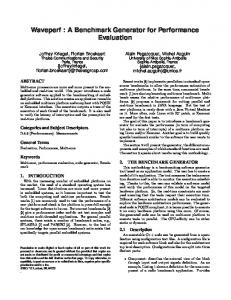
3 Experimental Results For the benchmark generation, 5 sequences are used. Each of the sequences contains 6 images like in the reference benchmark [3]. In Section 3.1, the resulting cost function values of different resolutions are compared. In Section 3.2 the evaluation protocol [3] is performed on the new data.

(a) Colors (b) Grace (c) Posters (d) There (e) Underground Fig. 2. First images of the input image sequences. The resolution is up to 3456 × 2304.

3.1 High-Resolution Benchmark Generation The resulting cost function values E(H) for the resolutions R1 = 1536 × 1024 and R2 = 3456 × 2304 are shown in Table 1. Two example sequences are selected, Grace and Underground. Due to the high accuracy of the computed homographies at resolution R2 , E(H) increases only slightly compared to resolution R1 . The generally larger error for the Underground sequence is due to the higher amount of light reflection from the surface of the wall. Nevertheless, the accuracies of the new homographies are high. Table 1. Comparison of cost function values E(H) for the homographies for image resolutions 1536×1024 (cf. [12] for Grace) and the new data set with resolution 3456×2304. The resulting cost function values for each image pair are approximately the same.

E(H) 1.5 megapixels 8.0 megapixels

Grace Underground 1-2 1-3 1-4 1-5 1-6 1-2 1-3 1-4 1-5 1-6 3.44 4.62 6.02 8.21 9.99 7.23 8.31 12.52 19.07 28.64 3.93 5.20 6.60 8.73 10.46 7.46 8.63 12.67 19.20 28.73

3.2 Repeatability Comparison To validate the usability of the new data set, the benchmark protocol provided in [3] is used. Like in Section 3.1, we compare results for resolution R1 = 1536 × 1024 with R2 = 3456 × 2304 for the sequences Grace (Figure 4) and Underground (Figure 3). Like in the majority of evaluation papers, the overlap error threshold is set to 40 %. The evaluated feature detectors are chosen from the reference paper [3]. Regarding the Underground sequence, the results for R2 are consistent with the results obtained for the smaller resolution R1 . MSER performs best followed by HessianAffine and IBR, very similar to the evaluation in [3] for the viewpoint change scenario. But, each of the detectors loose between 1 % and 9 % in repeatability. For the Grace sequence, the results are different for each detector. While HarrisAffine and Hessian-Affine perform like in the Underground sequence, MSER and IBR

K. Cordes, B. Rosenhahn, and J. Ostermann 90

90

80

80

70

70

60

60 repeatability %

repeatability %

332

50 40 30

Harris−Affine Hessian−Affine MSER IBR EBR

20 10 0 15

20

25

30

35 40 45 viewpoint angle

50 40

20 10

50

55

60

0 15

65

(a) Repeatability (1.5 megapixels)

20

25

30

35 40 45 viewpoint angle

50

55

60

65

(b) Repeatabality (8.0 megapixels)

5500

7000

5000

Harris−Affine Hessian−Affine MSER IBR EBR

4000

Harris−Affine Hessian−Affine MSER IBR EBR

6000

5000 nb of correspondences

4500

nb of correspondences

Harris−Affine Hessian−Affine MSER IBR EBR

30

3500 3000 2500 2000

4000

3000

2000

1500 1000

1000 500 0 15

20

25

30

35 40 45 viewpoint angle

50

55

60

65

(c) Correspondences (1.5 megapixels)

0 15

20

25

30

35 40 45 viewpoint angle

50

55

60

65

(d) Correspondences (8.0 megapixels)

Fig. 3. Repeatability results (top row) and the number of correctly detected points (bottom row) for the Underground sequence with different resolutions

significantly loose repeatability score. The repeatability rate of IBR decreases between 12 % and 15 % and MSER looses up to 25 % for large viewpoint changes. Interestingly, the EBR gains about 4 % for small viewpoint changes, but looses about 5 % for large viewpoint changes. Generally, none of the detectors can really improve their performance using high resolution images.

4 Conclusions In this paper, high-resolution image data of up to 8 megapixels is presented together with highly accurate homographies. This data can be used as a benchmark for computer vision tasks, such as feature detection. In contrast to the mainly used benchmark, our data provides high-resolution, fully planar scenes with removed radial distortion and a feature independent computation of the homographies. They are determined by the global optimization of a cost function using a dense representation of the images. The optimization is initialized with values inferred from the solution of lower resolution images. The evaluation shows that none of the standard feature detection approaches can improve in repeatability on higher resolution images. On the contrary, their performance

90

90

80

80

70

70

60

60 repeatability %

repeatability %

High-Resolution Feature Evaluation Benchmark

50 40 Harris−Affine Hessian−Affine MSER IBR EBR

30 20

Harris−Affine Hessian−Affine MSER IBR EBR

50 40 30 20

10

10

0 15

20

25

30

35 40 45 viewpoint angle

50

55

60

0 15

65

(a) Repeatability (1.5 megapixels)

20

25

30

35 40 45 viewpoint angle

50

55

60

65

(b) Repeatability (8.0 megapixels)

2000

3500 Harris−Affine Hessian−Affine MSER IBR EBR

1800 1600 1400

Harris−Affine Hessian−Affine MSER IBR EBR

3000

2500 nb of correspondences

nb of correspondences

333

1200 1000 800 600

2000

1500

1000

400 500 200 0 15

20

25

30

35 40 45 viewpoint angle

50

55

60

65

(c) Correspondences (1.5 megapixels)

0 15

20

25

30

35 40 45 viewpoint angle

50

55

60

65

(d) Correspondences (8.0 megapixels)

Fig. 4. Repeatability results (top row) and the number of correctly detected points (bottom row) for the Grace sequence with different resolutions

decreases. Dependent on the approach, the repeatability looses up to 25 %, but gains only 4 % in maximum. It follows, that feature detectors should be evaluated using high resolution images. The presented benchmark provides the necessary data to do this. The data set resulting from this work with all five sequences is available at: http://www.tnt.uni-hannover.de/project/feature_evaluation/ The provided resolutions include versions with 1.5 megapixels, 3 megapixels, 6 megapixels, and 8 megapixels for each sequence.

References 1. Mikolajczyk, K., Schmid, C.: Scale & affine invariant interest point detectors. International Journal of Computer Vision (IJCV) 60, 63–86 (2004) 2. Mikolajczyk, K., Schmid, C.: A performance evaluation of local descriptors. IEEE Transactions on Pattern Analysis and Machine Intelligence (PAMI) 27, 1615–1630 (2005) 3. Mikolajczyk, K., Tuytelaars, T., Schmid, C., Zisserman, A., Matas, J., Schaffalitzky, F., Kadir, T., Gool, L.V.: A comparison of affine region detectors. International Journal of Computer Vision (IJCV) 65, 43–72 (2005) 4. Schmid, C., Mohr, R., Bauckhage, C.: Comparing and evaluating interest points. In: IEEE International Conference on Computer Vision (ICCV), pp. 230–235 (1998)

334

K. Cordes, B. Rosenhahn, and J. Ostermann

5. Schmid, C., Mohr, R., Bauckhage, C.: Evaluation of interest point detectors. International Journal of Computer Vision (IJCV) 37, 151–172 (2000) 6. Haja, A., J¨ahne, B., Abraham, S.: Localization accuracy of region detectors. In: IEEE Conference on Computer Vision and Pattern Recognition (CVPR), pp. 1–8 (2008) 7. Tuytelaars, T., Mikolajczyk, K.: Local invariant feature detectors: a survey. Foundations and Trends in Computer Graphics and Vision, vol. 3 (2008) 8. Mikolajczyk, K., Schmid, C.: An affine invariant interest point detector. In: Heyden, A., Sparr, G., Nielsen, M., Johansen, P. (eds.) ECCV 2002, Part I. LNCS, vol. 2350, pp. 128–142. Springer, Heidelberg (2002) 9. F¨orstner, W., Dickscheid, T., Schindler, F.: Detecting interpretable and accurate scaleinvariant keypoints. In: IEEE International Conference on Computer Vision (ICCV), Kyoto, Japan, pp. 2256–2263 (2009) 10. Mobahi, H., Zitnick, C., Ma, Y.: Seeing through the blur. In: IEEE Conference on Computer Vision and Pattern Recognition (CVPR), pp. 1736–1743 (2012) 11. Brown, M., Lowe, D.G.: Invariant features from interest point groups. In: British Machine Vision Conference (BMVC), pp. 656–665 (2002) 12. Cordes, K., Rosenhahn, B., Ostermann, J.: Increasing the accuracy of feature evaluation benchmarks using differential evolution. In: IEEE Symposium Series on Computational Intelligence (SSCI) - IEEE Symposium on Differential Evolution (SDE). IEEE Computer Society (2011) 13. Matas, J., Chum, O., Urban, M., Pajdla, T.: Robust wide baseline stereo from maximally stable extremal regions. British Machine Vision Conference (BMVC) 1, 384–393 (2002) 14. Tuytelaars, T., Gool, L.V.: Wide baseline stereo matching based on local, affinely invariant regions. In: British Machine Vision Conference (BMVC), pp. 412–425 (2000) 15. Tuytelaars, T., Van Gool, L.: Content-based image retrieval based on local affinely invariant regions. In: Huijsmans, D.P., Smeulders, A.W.M. (eds.) VISUAL 1999. LNCS, vol. 1614, pp. 493–500. Springer, Heidelberg (1999) 16. Hartley, R.I., Zisserman, A.: Multiple View Geometry, 2nd edn. Cambridge University Press (2003) 17. Price, K.V., Storn, R., Lampinen, J.A.: Differential Evolution - A Practical Approach to Global Optimization. Natural Computing Series. Springer, Berlin (2005)