High-resolution measurements of the spatial and temporal scalar ...

Experiments in Fluids 31 (2001) 90±102 Ó Springer-Verlag 2001

High-resolution measurements of the spatial and temporal scalar structure of a turbulent plume J. P. Crimaldi, J. R. Koseff

90

sources, we need to determine the type of information that is conveyed to the animal by the temporal and spatial character of the odorant signal. An understanding of these processes might lead to an automated approach to locating the source of chemical signatures in the environment. The primary purpose of this paper is to describe two complementary experimental techniques for making highresolution measurements of the spatial and temporal structure of the scalar ®eld in turbulent ¯ows. We demonstrate the effectiveness of these techniques by measuring the structure of a scalar plume released from a low-momentum, bed-level, ¯ush source in a turbulent boundary layer. The results demonstrate that the techniques are capable of accurately measuring the spatial and temporal scalar structure over a wide range of scales in a complex turbulent ¯ow. 1 Both techniques described in this paper use a Introduction ¯uorescent dye as the scalar quantity, and they both rely Turbulent ¯ows continuously stir and mix embedded scalar quantities into complex and fascinating structures. on laser-induced ¯uorescence (LIF) to quantify the local dye concentration. The ®rst technique uses planar laserA detailed understanding of the physical processes that produce turbulent scalar diffusion relies on a description induced ¯uorescence (PLIF) to quantify the spatial scalar structure over a distributed region of the ¯ow. This techof the spatial and temporal structure of the scalar ®eld. nique produces highly resolved, 12-bit information about This has motivated the need for developing a variety of techniques for measuring scalar ®elds in the laboratory. A spatial structures, but data transfer rate and storage space second motivation for studying the spatial and temporal limitations preclude operating the PLIF technique fast structure of scalar ®elds (especially those in plumes) is to enough to fully resolve the temporal structure. The second understand what information the local structure conveys technique uses LIF to quantify the temporal scalar structure at a single point at kHz rates, trading off the spatial about the location of the scalar source itself. This originated in the area of olfaction, where a variety of aquatic coverage for high temporal resolution. Fluorescent dyes absorb excitation light over one range animals use chemoreception to locate the source of odors of wavelengths and then re-emit light over a second range emanating from food, predators, and potential mates of (longer) wavelengths. Under appropriate experimental (Weissburg and Zimmer-Faust 1993; Atema 1995). In conditions, the intensity of the ¯uoresced light, F, is order to be able to learn how the animals locate odor proportional to the local intensity of the excitation source, I, and the local concentration of the dye, C. The local Received: 8 May 2000/Accepted: 15 November 2000 excitation intensity can be reduced by attenuation (also called absorption, or quenching) of light by dye along the excitation path (Koochesfahani 1984; Walker 1987; Ferrier J. P. Crimaldi1 (&), J. R. Koseff Department of Civil and Environmental Engineering et al. 1993), and the local effective dye concentration can Stanford University, Stanford, CA 94305-4020, USA be reduced by bleaching of the dye by the excitation source (Saylor 1995; Crimaldi 1997). If the dye concenPresent address: trations are kept low enough, the absorption error is 1 Department of Civil, Environmental and minimized, and certain dyes (e.g., Rhodamine 6G) are Architectural Engineering, 428 UCB resistant to photobleaching; in this case, the local University of Colorado Boulder, CO 80309-0428, USA ¯uorescence is simply

Abstract Two techniques are described for measuring the scalar structure of turbulent ¯ows. A planar laser-induced ¯uorescence technique is used to make highly resolved measurements of scalar spatial structure, and a single-point laser-induced ¯uorescence probe is used to make highly resolved measurements of scalar temporal structure. The techniques are used to measure the spatial and temporal structure of an odor plume released from a low-momentum, bed-level source in a turbulent boundary layer. For the experimental setup used in this study, a spatial resolution of 150 lm and a temporal resolution of 1,000 Hz are obtained. The results show a wide range of turbulent structures in rich detail; the nature of the structure varies signi®cantly in different regions of the plume.

This work was supported by the Of®ce of Naval Research's F ˆ aIC …1† Chemical Plume Tracing Program, under Grants N00014-97-10706, N00014-98-1-0785 (Koseff) and N00014-00-1-0794 (Crimaldi). The authors would like to thank Megan Wiley for her where a is a spatially varying constant that can be deterexpert assistance with the data collection. mined empirically.

The PLIF experiments reported in the current study implement a unique calibration scheme that reduces or eliminates common sources of noise and errors and is simpler than existing approaches. The technique makes use of background dye in the image area to provide information to correct errors resulting from spatial variations in the pixel gain and dark response, laser scan nonuniformities, attenuation from background dye, lens vignette, and linear temporal trends in laser output, ¯ume temperature, and pH. Recent PLIF studies that used related techniques include Koochesfahani and Dimotakis (1985), Dahm et al. (1991), Brungart et al. (1991), Houcineet al. (1996), and Ferrieret al. (1993); the calibration and error correction approach used in these studies, however, differs from the approach presented here. A second technique used in the current study, a single-point LIF probe, enables a stock laser-Doppler anemometer (LDA) (common to many ¯uid mechanics laboratories) to be modi®ed in order to make high-resolution measurements of temporal scalar structure. Related approaches have been described by Durst and Schmitt (1984), Walker (1987), and Lemoine et al. (1999). We use the techniques presented in this paper to investigate the scalar structure of a neutrally buoyant plume in a turbulent boundary layer. The plume source emanates from a 1-cm circular region that is ¯ush with the bed, and the momentum associated with the scalar release velocity is extremely low. The source geometry is designed to mimic a diffusive odorant release from a source that is buried below a smooth substrate. To our knowledge, the structure of plumes resulting from this type of source geometry have not been previously reported in the literature. There are, however, a number of existing studies involving plume structure from a variety of different source types. Two studies involving neutrally buoyant plumes released from ground-level sources into turbulent boundary layers are particularly relevant to the current study. Fackrell and Robins (1982) used a ¯ame ionization system to study plumes released from various heights in a wind tunnel. A 1.5-cm-diameter horizontal tube released the odorant iso-kinetically (jet velocity matched the local ¯ow velocity) into the ¯ow at one of two vertical locations (one of which was just above the bed). Bara et al. (1992) used a conductivity probe to study plumes over rough surfaces in a water ¯ume. A 0.536-cm-diameter horizontal tube placed on the bed released the odorant. In both of these studies, the source release involves a signi®cant amount of (horizontal) momentum, and the release is distributed over a large (relative to the inner boundary layer scales) vertical distance. Shlien and Corrsin (1976) performed a study with a thermal release from a long, thin, heated wire located at the wall (and other locations), but presents only mean temperature results. Several analytical and numerical studies are also relevant to the current study: Robins (1978), El Tahry et al. (1981), and Hanna (1984) all discuss the statistics of scalar dispersal in turbulent boundary layers. The layout of the remainder of this paper is as follows. The PLIF and LIF techniques themselves are described in Sect. 2. An application of the techniques to measure the scalar structure of odor plumes with ¯ush-mounted,

low-momentum sources is described in Sect. 3, with some sample results presented in Sect. 4. Finally, a discussion of scale and resolution issues is given in Sect. 5. The paper concludes in Sect. 6 with a summary of our ®ndings.

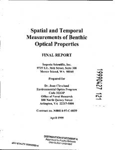
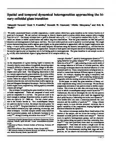
2 Description of the techniques 2.1 Spatial measurements 2.1.1 Imaging apparatus The imaging apparatus consisted of an argon-ion laser, optics for focusing and scanning the laser beam across the image area, and a digital camera. An image was acquired using the following sequence: (1) the camera began exposing the CCD chip, (2) an optical scanner scanned the focused laser beam across the image area in a single, unidirectional pass, (3) the camera stopped exposing the CCD chip, and (4) the optical scanner returned the laser beam to the original location (just beyond the edge of the image area). A delay was introduced between steps (3) and (4) to allow suf®cient time for the camera to shift the image off the chip without exposure contamination from the returning laser beam. All of the steps in the sequence were controlled by analog and digital signals generated by a computer running a LabView program. The laser used was a Coherent Innova 90, operated in a single-line mode at k ˆ 514.5 nm (green) at 1.3 W in a closed-loop light-regulated mode. The laser beam exits the laser head with a diameter (measured at the e)2 intensity location) of dexit ˆ 1.5 mm. Rhodamine 6G was used as the ¯uorescent dye (the ``odorant''). In water, Rhodamine 6G has a central excitation (absorption) wavelength of kex ˆ 524 nm, and a central emission (¯uorescence) wavelength of kem ˆ 555 nm (Penzkofer and Leupacher 1987). Both the excitation and emission spectral peaks have bandwidths of approximately 40 nm. The 514.5 nm line of an argon-ion laser is, therefore, an effective excitation source for the dye. Barrett (1989) reports that Rhodamine 6G has a Schmidt number of 1,250. Figure 1 shows the con®guration of the optics used to focus and scan the laser beam. The con®guration shown is for a horizontal laser scan (parallel to the bed); the laser enters the water through the side wall of the ¯ume. Vertical laser scans were also used; for these scans the laser entered the water through a thin glass plate placed on the free surface of the water. In order to increase the spatial resolution in the direction normal to the laser scan, the laser beam was focused using a Melles Griot 6´ beam expander in conjunction with a f ˆ 2,000 mm focusing lens as shown in Fig. 1. A conservative estimate for the focused beam waist diameter, d, is given by the formula dˆ

2:44kf dexit

…2†

The focused beam waist diameter for our optical setup, calculated using Eq. (2), is thus 0.28 mm. The focused beam waist has a ®nite depth-of ®eld; however, for a

91

tensity measured at a plane normal to the beam is IB ˆ 4P/ pd2. The intensity measured in a plane that is at an angle h to the normal is IBcosh. The CCD chip on the camera integrates the laser intensity at a point over the time interval of the exposure, T. The optical scanner was programmed such that the transit time for a single laser beam scan (from )hS/2 to hS/2) is equal to the camera exposure integration time, T. A given pixel on the CCD chip is exposed to darkness during the majority of the exposure period; the actual exposure occurs during the relatively short time period when the laser beam transits the pixel location.1 The time-averaged intensity of the laser beam (over the duration of a single scan) at any location depends on the scan rate oh/ot. Along a straight line located at y ˆ D (refer to Fig. 2), the average intensity of the scanned beam is

92

IE …h† ˆ IB Fig. 1. Optical arrangement for scanning a focused laser beam across the image area (horizontal scan con®guration shown)

d cos2 h D T oh ot

…3†

The total exposure seen by the camera at any location h along the line y ˆ D is then IE(h)T. It is desirable to typical 15-cm image size, the beam diameter at the edge of minimize the variation in IE(h)T across all of the pixel locations; as the light sheet becomes more uniform, the the image is estimated still to be less than 0.5 mm. The focused laser beam was scanned across the image correction algorithm becomes less sensitive to errors rearea using a moving-magnet optical scanner (Cambridge sulting from changes in image alignment. For a constant angular rate (oh/ot ˆ constant), the exposure along the Technology model 6800HP). The scanner consists of a line y ˆ D (corresponding to a line of pixels on the CCD square 5-mm mirror actuated by a closed-loop galvachip) varies as cos2h. Because the optical scanner used in nometer; the manufacturer reports an angular step-response time of 0.3 ms and an angular positioning accuracy these experiments is not constrained to move at a constant angular rate, we removed the non-uniform exposure along of 20 lrad. 2 Figure 2 contains a sketch of the geometry of the laser the line y ˆ D by setting oh/ot ˆ (1/T)cos h. The resulting beam as it is scanned across the image area by the optical command signal to the mirror is then based on   scanner (labeled ``OS''). A focused cylindrical laser beam hS 2t T arctan …4† with power P and diameter d is shown exiting the mirror at h…t† ˆ p=4 T an angle de®ned as h. For a stationary laser beam, the inAlthough there is still a 1/D dependence in the exposure along lines x ˆ constant, there is no way to correct out this variation with the mirror command. However, this exposure variation is removed during the image processing, as described in Sect. 2.1.2. The camera is manufactured by Silicon Mountain Design (model SMD-1M15). This scienti®c-grade camera is based on a 1,024 ´ 1,024 pixel CCD chip with true 12-bit gray scale intensity resolution. The ability to measure a large number of intensity scales (4,096 for this camera) is important for imaging instantaneous odor plume structures due to the high dynamic range of the scalar intensity ¯uctuations present in each image. A ¯at-®eld lens (MicroNikkor, f ˆ 55 mm) was used, and the lens was ®tted with a narrow bandpass optical ®lter (center wavelength ˆ 557 nm, bandwidth ˆ 45 nm).

2.1.2 Image acquisition and processing For a given image location and ¯ow condition, a time series of images An …i; j† are acquired from the camera. 1 The duration of the single-pixel exposure time is the quotient of the projected beam width d/cos h and the x-direction beam 2 Fig. 2. Schematic of the laser beam geometry as translated by the translation velocity D oh ot sec h, where D and h are as de®ned in optical scanner Fig. 2.

Typically, 8,000 images are acquired (1 £ n £ 8,000), and each image is a 1,024 ´ 1,024 array of numbers (1 £ i £ 1,024, and 1 £ j £ 1,024). The information content in these images is a linear superposition of ¯uoresced light from the odorant structures, ¯uoresced light from the background concentration of odorant in the ¯ume, and the dark-response of the camera. The content associated with ¯uoresced light is linearly related to the total odorant concentration and laser intensity at each point. The content in the nth image can be expressed symbolically as

An …i; j† ˆ an …i; j†In …i; j†A0n …i; j† ‡ In …i; j†bn ‡ D…i; j† …5† where an(i,j) is the spatial distribution of the ¯uorescence constant of proportionality, In(i,j) is the spatial distribution of the average laser intensity in the image area during the laser scan, A0n …i; j† is the spatial distribution of the odorant intensity (not including the background odorant), D…i; j† is the spatial distribution of the darkresponse of the camera, and bn is the value of the background concentration. The background concentration results from initial dye in the ¯ume, plus the continual addition of dye from the plume source. The water in the test section (along with the embedded dye structures) empties into a downstream mixing reservoir before being recirculated back into the ¯ow. The mixing in the reservoir ensures that the background concentration is spatially uniform but, because of the recirculation, the background concentration levels increase with time. For the plume dose rates and experiment durations used in these studies, the background concentration growth is highly linear in time. Associated with each image An …i; j† is a background image Bn …i; j† acquired from the camera under identical conditions except for the absence of the odor plume. As described below, the associated background images at any time during the experiment are interpolated from two background images taken before and after the experiment. The content in the nth background image can be expressed symbolically as

Bn …i; j† ˆ an …i; j†In …i; j†bn ‡ D…i; j†

…6†

Equations (5) and (6) contain the term an(i,j), which relates the measured ¯uorescence intensity to the excitation intensity. The value of an(i,j) is unknown; it depends on temporal and spatial ¯uctuations in pH, temperature, CCD response, optical transmission, and other factors. Combining Eqs. (5) and (6), and solving for A0n …i; j† gives

A0n …i; j† ˆ bn

An …i; j† Bn …i; j†

Bn …i; j† ; Dn …i; j†

…7†

which eliminates any explicit reference to an(i,j) in the formulation. Equation (7) represents the core of the algorithm that is implemented to process the images from the camera. The algorithm removes the background ¯uorescence and the dark response, and then corrects for variations in the light sheet intensity and an(i,j). The spatial calibration of the images is accomplished by using an image of a graduated scale placed in the image plane prior to each experiment.

In practice, only two background images are acquired for each experiment: one image is taken at the beginning of the experiment (before image A1 ), and one is taken at the end of the experiment (after image A8000 ). A ¯uorometer is used to record the background concentration in the test section during each individual image acquisition. Flume water is extracted upstream of the test section and passed through a ¯ow-through cell in the ¯uorometer. The residence time in the ¯uorometer bypass plumbing is designed to match the residence time of the associated ¯ow through the test section, ensuring that the ¯uorometer is measuring ¯uid that is representative of the ¯ow currently in the test section. An RS-232 connection enables the ¯uorometer to be sampled every time an image is acquired. The ¯uorometer data are also strongly linear in time; the data are used to obtain a series of virtual images Bn …i; j† from the two real background images using interpolation. This practice enables the dye source to be run continuously during the acquisition of the images An …i; j†. A single dark-response image is acquired after each experiment. So as not to rely on the ¯uorometer calibration for the image calibration, the processed images are re-calibrated using a mean odorant concentration value obtained from the LIF probe (see Sect. 2.2) for a single pixel location within each image area for each experiment. This LIF data point serves to set the slope of a two-point calibration (where the two background images serve to set the zero point of the calibration). Then, Eq. (7) takes care of the pixel-to-pixel variations in the calibration process. Note that such a two-point calibration approach is feasible due to the high linearity of the camera response and the ¯uorescence physics for the chosen conditions. The processed instantaneous images, A0n …i; j†, can be used to calculate statistical information about the spatial structure of the concentration ®eld. In Sect. 4, we present the spatial distributions of the mean concentration, root mean square (rms) concentration ¯uctuation intensity, and concentration intermittency.

2.1.3 Error sources and corrections Errors in the image acquisition system stem from spatial and temporal variations in the excitation laser scan intensity [In(i,j)], dye ¯uorescence capability [an(i,j)], and camera response [also carried in an(i,j)]. Many of these errors can be corrected by the algorithm given in Eq. (7). However, because of our choice to acquire only two background images per experiment (and to obtain virtual background images by interpolation for the correction algorithm, based on continuous ¯uorometer data), only spatial variations that are constant in time during the experiment are completely corrected. Some slowly varying spatial variations are also corrected, depending on their effect on the system, but our approach was to minimize temporal variations directly whenever possible (the biggest exception being the background concentration growth, which is directly corrected through the algorithm). Spatial variations in the excitation laser scan intensity result primarily from the nature of the laser scan generation, as discussed previously. The variation in the

93

94

streamwise direction was removed directly through the choice of the command signal sent to the optical scanner, but it is not possible to remove the cross-stream variation. Fortunately, the scan intensity varies smoothly in space, and is constant in time, so Eq. (7) successfully corrects for this variation, so long as the camera alignment is maintained during the course of the image acquisition sequence. The presence of dye in the test section also alters the scan intensity across the light sheet through an attenuation process (Koochesfahani 1984; Walker 1987; Hannoun and List 1988; Ferrier et al. 1993). Since the background dye is well mixed in the test section (and this dye is the source for the measurements used for the background image interpolation), the attenuation from background dye is completely corrected for by Eq. (7). However, the presence of higher concentration structured dye in the plume is a potential cause for concern. Koochesfahani (1984) describes a correction algorithm for attenuation due to rapidly varying dye structures; this approach is based on the well-known Beer±Lambert law given by

0

I…r; h† ˆ exp@ e I0

Zr

1

C…r; h†dr0 A

…8†

r0

where I(r,h) is the local beam intensity (the coordinate r is measured radially from the scanning mirror), I0 is the beam intensity at the location where the beam enters the dyed ¯uid (at r ˆ r0), C(r,h) is the local instantaneous dye concentration, and e is the extinction coef®cient for the dye. However, the Beer±Lambert attenuation correction approach is numerically expensive for 2-D image data produced with a radial-scan light sheet; a simpler approach is to minimize the dye concentrations so that the magnitude of the error is acceptable. The magnitude of the attenuation error depends on the scale and intensity of concentration ®laments. The worst attenuation in our experimental setup occurs close to the source, where concentration peaks can be large (often several orders of magnitude higher than the local mean concentration). At x ˆ 40 cm (the closest location to the source at which data are reported in this paper), the highest concentration peak recorded in a 30-min record for the 10 cm/s ¯ow speed was C/C0 ˆ 0.068, or, dimensionally 1.36 ppm. Using the extinction coef®cient 23 (ppm m))1 reported by Ferrier et al. (1993) for Rhodamine 6G, this results in a 3.7% error due to the attenuation in the determination of the magnitude of this single peak. More typical peaks (occurring 100 times in 30 min) had concentrations of C/C0 ˆ 0.02, with an associated attenuation error of 1.1%. However, these errors apply only to the determination of the magnitude of the individual peaks themselves. If the Beer±Lambert law is used to manually attenuate the entire recorded concentration history at x ˆ 40 cm, the mean concentration changes by only 0.23%, the rms ¯uctuation changes by only 0.86%, and the effect on the measured intermittency is negligible. Furthermore, the magnitude of the concentration peaks at other reported locations, and for the higher ¯ow speed, are far lower, with associated attenuation errors that are also far lower. Due to

the minimal effect of attenuation on the concentration statistics, we chose not to perform the Beer±Lambert correction associated with Eq. (8) in order to reduce processing time. Temporal variations in the laser output power would also cause measurement error. The laser was operated in a closed-loop light regulation mode in order to minimize this source of error. The rms noise level of the laser output is 0.2%, and the long-term stability of the laser output is rated at 0.5%. Even if the laser output power does drift during the course of an experiment, the linear trend component of the drift would be removed by Eq. (7). Changes in the propensity of the dye to ¯uoresce under a given excitation level are another potential source of error. The ¯uorescence of Rhodamine 6G, like most dyes, is pH and temperature-dependent. Care was therefore taken to hold these quantities constant during an experiment. Additional ¯uorescence is obtained with time due to growth of background dye concentration in the recirculating ¯ume. This effect is corrected by Eq. (7). Another ¯uorescencerelated concern is the process of photobleaching, whereby the dye loses some of its ability to ¯uoresce under strong excitation (Sugarman and Prud'homme 1987; RieÁka 1987; Saylor 1995; Crimaldi 1997). Rhodamine 6G was chosen for this study because it has been shown by Crimaldi (1997) to be resistant to photobleaching. Like attenuation, photobleaching would manifest itself as an asymmetry in the odor statistics, which was not observed. The ®nal sources of error are associated with the camera itself. Optical effects such as lens vignette or variations in optical transmission by the ¯ume walls can change the measured ¯uorescence. The same is true for spatial (pixelto-pixel) variations in the response of the CCD chip. The CCD chip also has a dark response which must be removed. All of these error sources are presumed to be constant in time, and hence completely corrected by Eq. (7). The potential error sources and corrective actions taken are summarized in Table 1. Table 1. Summary of error sources and corrections Error source

Correction Eq. (7)a

Laser scan intensity pattern Attenuation (background dye) Attenuation (plume dye) Laser power Flume pH Flume temperature Background ¯uorescence Photobleaching Optics (lens vignette, ¯ume walls) CCD pixel variation CCD dark response a

´ ´ ´ ´ ´ ´ ´ ´

None

´b ´c

´d

Equation (7) corrects only steady or slowly varying spatial variations in the listed error sources due to the use of the interpolated background image b Mitigated through minimizing concentrations; symmetry of results indicates that error was not signi®cant c Laser operated in closed-loop light regulation mode d Eliminated through choice of dye

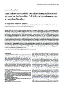
2.2 Temporal measurements A second measurement technique, a laser-induced ¯uorescence (LIF) probe, was used to independently measure concentration time-histories at selected points in the odor plume. Although the LIF probe can only record concentration information at a single point, the probe can resolve temporal ¯uctuations in the concentration history up to 1000 Hz. The LIF probe is a custom addition to a stock Dantec 2-D laser-Doppler anemometer (LDA) system. The complete system is capable of making simultaneous measurements of concentration and velocities (see Crimaldi 1997, 1998 for additional information). The LIF probe measures dye ¯uorescence at the intersection of three 514.5-nm laser beams that are focused to a point by the LDA optics, as shown in Fig. 3. The resulting measurement volume is approximately 0.1 mm in the streamwise (x) and vertical (z) directions, and 1 mm in the cross-channel (y) direction. Dye passing through the LIF measurement volume ¯uoresces with an intensity that is proportional to its concentration; the ¯uoresced light is gathered by a set of back-scatter optics and the intensity is measured using a photomultiplier tube (PMT). A closed-loop high-voltage power supply is used to provide a stable voltage to the PMT. The PMT current is converted to a voltage using an ideal currentto-voltage converter, and the resulting voltage is recorded by an A/D card in a PC. The LIF probe is calibrated by ¯ooding the LIF measuring volume with a known concentration of dye. This calibration is done in-place in the ¯ume test section, with the appropriate background concentration levels in the ¯ume. A horizontal 1-cm stainless steel tube is place directly upstream of the LIF measuring volume, and a know concentration of dye is pumped (iso-kinetically) through it. The LIF measuring volume is placed close enough to

Fig. 3. Schematic of the LIF probe system used to measure the temporal structure of the odor plume at a point

the tube exit such that the measuring volume remains in the potential core of the jet ¯ow. A 0.15 PPM concentration calibration solution was used (this exceeded the mean concentration of the local plume structure to be determined with the probe). The path length through the calibration concentration solution is only 0.5 cm, which results in a raw calibration error of 1.1%; this error can be corrected using the Beer±Lambert law as described earlier.

3 Application of the techniques We created a laboratory-scale odor plume within a turbulent boundary layer along the bed of a recirculating ¯ume. A ¯uorescent dye was used as the scalar odorant; it was released from a low-momentum source ¯ush with the bed at the upstream edge of the ¯ume test section. The full-®eld PLIF technique and the single-point LIF techniques were used to quantify the spatial and temporal structure of the resulting plume. 3.1 Flow facility We used the two techniques described above to measure the spatial and temporal structure of a laboratory scale odor plume. The experiments were conducted in an open-channel recirculating ¯ume with a test section that is 3 m long and 0.6 m wide. The ¯ume is driven by a digitally controlled pump that ®lls a 4-m-high constanthead tank; this arrangement allows for constant and repeatable ¯ow conditions in the test section. Water from the constant-head tank enters the ¯ume and passes through a diffuser, three homogenizing screens, and a two-dimensional contraction before entering a rectangular channel section. A 3-mm-diameter rod spans the ¯ume ¯oor at the start of the channel, serving as a boundary layer trip. The boundary layer develops over a 2.2 m distance before encountering the plume source in the test section. The bed of the ¯ume is Plexiglas, with no roughness elements. The ¯ow depth in the test section is approximately 0.25 m, and the d99 thickness of the momentum boundary layer is approximately 0.10 m, depending on the ¯ow condition. The turbulence levels are approximately 2%, and the test section is free from arti®cial secondary ¯ows due to the entrance section, residual pump vorticity, etc. A more detailed description of the ¯ow facility is given by O'Riordan et al. (1993) and Crimaldi (1998). The walls of the test section are made of glass to improve optical clarity. The ¯oor is made of Plexiglas that has been painted black to minimize laser re¯ections. A small glass window can be placed on the free surface of the ¯ow to enable optical access for the laser sheet in the vertical con®guration; this window does not alter the ¯ow in the image area. A sketch of the ¯ume test section is shown in Fig. 4. Results are presented for two ¯ow conditions; the mean freestream velocities for the two ¯ow conditions are U1 ˆ 10 cm/s and U1 ˆ 30 cm/s, respectively. Hydrodynamics details of these ¯ow conditions can be found in Table 2 and in Crimaldi (1998).

95

bed in the ¯oor of the ¯ume. The hole is ®lled with a porous foam that is designed to provide a uniform ¯ow across the source exit; the foam is mounted ¯ush with the bed of the ¯ume. A small gear pump is used to pump the dye solution through the odor source at a volumetric rate of 3 ml/min, resulting in a vertical exit velocity of Ws ˆ 0.063 cm/s. The electronic gear pump provides an accurate dose rate with no measurable pulsing.

96 Fig. 4. Side view of the ¯ume test section showing the odorant source location and coordinate system (vertical laser scan con®guration shown) Table 2. Experimental ¯ow conditionsa U1 [cm/s]

us [cm/s]

d [cm]

Reh

10 30

0.488 1.18

9 9

540 1.79 ´ 103

a

All values were measured on the ¯ume centerline at x = 170 cm

3.2 Odor source design The odor source is designed to mimic a diffusive-type (i.e., low-momentum) release of a scalar from a ¯ush, bed-level source in a turbulent boundary layer. The odor source is located on the ¯ume centerline, near the upstream edge of the test section (2.2 m downstream of the boundary layer trip). The odor source location is designated x ˆ 0. A 20 ppm aqueous solution of the laser ¯uorescent dye Rhodamine 6G is used as the scalar odorant. The dye solution is pumped slowly through the odor source, which is a 1-cm-diameter circular hole drilled perpendicular to the

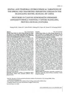
4 Results A sample image showing the instantaneous spatial structure of an odor plume is shown in Fig. 5. The image shows a vertical slice in the x±z plane on the plume centerline (y ˆ 0), in the vicinity of x ˆ 100 cm. The concentrations are normalized by the source concentration, C0, and a falsecolor scheme is applied to the image. The image clearly shows some of the well-known structural features of a turbulent momentum boundary layer: the viscous sublayer (VSL) is made visible because of its propensity to trap dye; turbulent burst structures are then visible because they take dye-laden ¯uid from the VSL into the overlaying ¯ow; sweep structures, on average, tend to contain less dye. The image also illustrates some of the structural features of the scalar boundary layer: the dye is stirred into highly ®lamentous structures by the boundary layer vorticity; this stirring action places thin ®laments of high-concentration structures very close to regions of near-zero concentration ¯uid and mixing ensues. Another feature is odorant intermittency: the mean concentration results from very strong odorant structures that occur, on average, very infrequently. Note that the instantaneous red odorant structure near x ˆ 108 cm, z ˆ 6 cm has a concentration that is over 500 times the mean concentration at that location. A long series of images such as that shown in Fig. 5 can be ensemble-averaged to calculate odorant statistics. Instantaneous concentrations, C, are decomposed into the  and the ¯uctuating sum of the mean concentration, C,

Fig. 5. Instantaneous concentration ®eld in a vertical slice through the plume centerline (y ˆ 0). Concentrations are normalized by the source concentration C0

Fig. 6. Mean concentration ®eld in a horizontal slice at z ˆ 2 cm. Concentrations are normalized by the source concentration C0. The image is a mosaic of ®ve separate sub-images

concentration, c. The mean concentration ®eld in a horizontal slice at z ˆ 2 cm is shown in Fig. 6. The image is actually a mosaic of the mean image from ®ve series of images at different streamwise locations. Because the slice is taken above the bed, the mean concentration at x ˆ 0 is zero. The mean concentration reaches a peak near x ˆ 65 cm and decays downstream from there. Normalized mean lateral concentration pro®les at several streamwise and vertical locations and for both the U¥ ˆ 10 cm/s and U¥ ˆ 30 cm/s ¯ow cases are shown in Fig. 7. The values of Cm and ry are obtained from a twoparameter least-squares ®t to the equation

C y2 ˆ exp 2r2y Cm

!

…9†

Figure 7 also contains a plot of Eq. (9), although it is dif®cult to see amongst the symbols. The mean lateral concentration pro®les are clearly Gaussian and self-similar, in agreement with previous plume studies by Fackrell and Robins (1982) and Bara et al. (1992). The symmetry and Gaussian shape of the data are indicative of the accuracy of the technique, and of the ability of the image processing method (as described in Sect. 2) to ensure uniform results over the entire ®eld of view of the image. Furthermore, the near-zero mean concentration values far from the plume centerline demonstrate the absence of any mean zero-level bias in the technique.

97 The strength of concentration ¯uctuations can be quanti®ed by the rms value
of the ¯uctuations, c¢, or the 1=2 variance, c2 , where c0 ˆ c2 . Figure 8 contains an image of the normalized rms concentration ¯uctuation strength c¢ in a horizontal slice at z ˆ 2 cm near x ˆ 100 cm. Note that the fuzziness in the image is not noise. Even with 8,000 images used to calculate this statistic, the result is not fully statistically converged; individual structures that contributed to the rms strength are still visible in the image, producing the fuzzy texture. It is possible to view structures near the edges of the plume that occurred only once at a given location during the entire sampling period. For the horizontal slice shown, c¢ has reached a maximum upstream of the image, and is decaying in the downstream direction. Normalized lateral pro®les of c¢ at several streamwise and vertical locations for both ¯ow cases are shown in Fig. 9. The values for c0m and ry were obtained by ®tting c0 =c0m to the right-hand side of Eq. (9); once again, Eq. (9) is included in the ®gure, but it is dif®cult to discern. The lateral pro®les of concentration c¢ shown in the ®gure are strongly Gaussian, with no evidence of off-axis bipolar maxima. Some previous boundary-layer plume studies (Fackrell and Robins 1982; Bara et al. 1992) did report offaxis variance peaks, but the source conditions for those studies differ substantially from those in the current study (the previous studies used iso-kinetic jet sources rather than ¯ush, low-momentum sources). Hanna (1984) suggests that the concentration variance may have a single centerline peak for certain plume types, in agreement with the results presented here. The near-zero values of c¢ far from the plume centerline are indicative of the extremely low intrinsic noise level that the technique described in this paper is capable of producing. Another statistical measure of the plume structure is the odorant intermittency, c, de®ned herein as

c ˆ prob‰C > CT Š

Fig. 7. Normalized lateral pro®les of mean concentration. Units in the legend are in terms of cm. The solid line is the Gaussian  m ˆ exp… y2 =2r2 † C=C y

…10†

where CT is a concentration threshold value; the choice of this parameter involves some arbitrariness, as discussed in detail by Chatwin and Sullivan (1989). For the results presented here, we have chosen CT ˆ 0.0002C0. Figure 10 contains an image of the concentration intermittency in a horizontal slice at z ˆ 2 cm near x ˆ 100 cm (the same location as shown in Fig. 8). The intermittency is growing slowly in the streamwise direction as the turbulent mixing process breaks down sharp odor ®lament gradients into

98

Fig. 8. Rms concentration ¯uctuation strength in a horizontal slice at z ˆ 2 cm near x ˆ 100 cm. The ¯uctuation strengths are normalized by the source concentration C0

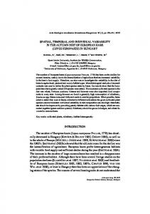
A single-point LIF probe, as discussed earlier, was used to measure the temporal structure of the plume. Figure 12 shows a 20-s record of the odorant concentration for the U1 ˆ 10 cm/s ¯ow condition at x ˆ 40 cm, z ˆ 2 cm. The intermittent nature of the odorant signal is clearly visible. The temporal structure of the odorant signal is characterized by odorant bursts with fast rise times and of short duration. The time history shows the extremely fast temporal response of the LIF probe, and the ¯at zero-concentration periods between odorant bursts are indicative of the low noise level and lack of zero-level bias associated with the technique. The concentration spectra of much longer records for the U1 ˆ 10 cm/s and U1 ˆ 30 cm/s ¯ow conditions at this same location are shown in Fig. 13. The LIF probe resolves nearly six decades of concentration ¯uctuations, Fig. 9. Normalized lateral pro®les of rms concentration ¯uctuawith frequency contents above 1000 Hz. tion strength. Units in the legend are in terms of cm. The solid line is the Gaussian c=c0m ˆ exp… y2 =2r2y †

5 Scales and resolution For the measurement of an odor plume, three scales must be addressed: the spatial, temporal, and odor intensity scales of the instantaneous odor structure. An accurate quanti®cation of the odor structure relies on adequate resolution of all three of these scales. The smallest spatial scales of motion in the ¯ow are set by the Kolmogorov scale, which can be estimated in the log-law region of the boundary layer as  3 14  3 14 m jzm gK ˆ  …11† e u3s

more diffuse structures. Near the centerline of the plume, odorant concentrations above CT are present nearly 50% of the time. Normalized lateral pro®les of c at x ˆ 100 cm for three vertical locations for both ¯ow cases are shown in Fig. 11. The values for cm and ry are obtained by ®tting c/cm to the right-hand side of Eq. (9). Equation (9) is included in the ®gure as a solid line. Also shown in the legend of the ®gure is the value of cm associated with each intermittency curve. In general, the lateral pro®les of concentration intermittency are not Gaussian. The deviation away from the Gaussian shape becomes more extreme in ¯ow locations and conditions where cm ® 1; these locations also have an For weakly diffusive scalars (Sc ˆ m=D  1), concentraassociated clipped concentration pdf. tion ¯uctuations can exist on scales smaller than the

99

Fig. 10. Concentration intermittency in a horizontal slice at z ˆ 2 cm near x ˆ 100 cm. The threshold used to calculate the intermittency is 0.0002C0

Fig. 11. Normalized lateral pro®les of concentration intermittency at x ˆ 100 cm. The solid line is the Gaussian c=cm ˆ … y2 =2r2y †

Kolmogorov scale. The smallest scalar ¯uctuations are set by the Batchelor scale, given by Batchelor (1959) as

gB ˆ gK Sc

1=2

…12† +

For the U¥ ˆ 10 cm/s ¯ow case at z ˆ 0.7 cm (z ˆ 30), Eqs. (11) and (12) give gK ˆ 0.4 mm and (for Sc ˆ 1,250) gB ˆ 0.01 mm. Of course, there are smaller odor ¯uctuation scales very close to the wall, but this estimate of gB is representative of the typical small odor scale for most of the data reported here. The spatial resolution of the PLIF imaging system is set primarily by the quotient of the image dimension and the array size of the CCD chip in the camera. The (square) image dimensions used for this study were approximately

Fig. 12. Normalized concentration time-history output from the LIF probe for the U¥ ˆ 10 cm/s ¯ow case at x ˆ 40 cm, z ˆ 2 cm

15 cm for the images in the vertical plane and 30 cm for horizontal images; for the 1,024 ´ 1,024 pixel array, this results in a spatial resolution range of 0.15±0.29 mm in the plane of the laser scan. The spatial resolution normal to the plane of the laser scan depends on the out-of-plane width of the laser scan; the high resolution produced from a small image dimension and large pixel array size can be corrupted by the spatial integration of structure through a thick laser sheet. For our setup, a conservative estimate for the out-of-plane spatial resolution in the central region of the sheet was calculated to be 0.28 mm. Thus, for a 15 cm image dimension, a single-pixel integration volume has dimensions of 0.15 mm on a side (about 0.4gK or 13gB) in the plane of the laser scan, and a dimension of 0.28 mm normal to the laser scan. Thus, it would be necessary (and possible) to reduce the total image size in order to capture

100

Fig. 13. Concentration spectra calculated from LIF data for two different ¯ow conditions at x ˆ 40 cm, z ˆ 2 cm

the smallest odorant scales. However, we chose the image size based on a compromise between capturing the smallest scales while still being able to record the largescale odorant structure. Errors can be introduced into the measured values of odor concentration statistics if the integration volume is overly large. The mean concentration is generally the statistic that is the least susceptible to resolution-based errors. If the measurement volume dimension in the xi direction is denoted by di, then resolution-based errors in the mean concentration can be avoided by ensuring that

 C di   …13† oC=oxi  varies reasonably slowly for most parts of the Because C plume, this criterion is generally easy to meet. Even though there may be instantaneous concentration structures that are substantially smaller than the pixel scale, the camera pixel performs a spatial and temporal integration on the small moving structure with no introduced error on the resulting mean concentration. The integration volume size becomes more critical for higher-order statistics such as concentration variance (or rms concentration) or intermittency. If di  gB , then the measured variance will be arti®cially low due to spatial smearing of sub-pixel-scale structures (although the effect may be minimal since the majority of the variance is contained in the larger integral length scale eddies). Conversely, the measured intermittency will be arti®cially high when di  gB , although the degree of error depends on the characteristics of the instantaneous concentration structure and on the true value of the intermittency itself (as ctrue ® 1, the resolution-based intermittency error disappears). In general, resolution-based errors will be largest where there is a prevalence of high-concentration, smallscale features in the concentration ®eld, e.g., close to the source but not close to the bed. In these regions, the turbulence has stirred the odorant into ®ne-scale structures, but the odorant structures are still distinct and relatively unmixed. Further downstream and/or close to the bed, the

turbulence has stirred the odorant to such small scales that molecular diffusion has eradicated much of the small-scale structure, thus relaxing the integration volume dimension criterion. The spatial resolution of the imaging system is also governed by temporal considerations. The spatial resolution of a moving odor structure can be corrupted by temporal integration during the exposure sequence. The single-scan laser imaging system used in this study was designed to minimize distortion and smearing due to temporal averaging. The duration of a laser scan across the entire image area ranged from 8 ms to 250 ms (depending on the ¯ow condition and image location), with a typical scan having a duration of 50 ms. For a typical advective ¯ow speed of 10 cm/s, the odor structures illuminated at the end of the scan (at one edge of the image) would have moved, on average, 0.5 cm from where they were located when neighboring odor structures at the beginning of the scan were being illuminated (15 cm away at the opposite edge of the image). This results in a potential 3% spatial distortion from one edge of the image to the other. However, the largest odor structure scales are typically much smaller than the image size, so this potential distortion is unlikely to affect coherent structures. Much more important is the spatial resolution at pixel-level scales. In a traditional continuous light sheet (made with a cylindrical lens or multiple scans of a rotating mirror), a given pixel integrates odorant over the entire exposure period (which is necessarily long since the available laser power is spread out over a large area). This results in a spatial smearing of pixel-scale odor structures if the distance that they advect during the exposure time is comparable to or larger than the single-pixel image dimension. For the single-scan laser system used for this study, a given pixel is exposed for a time approximately equal to 1/1,024 of the total scan time across all of the pixels. This small pixel exposure time provides suf®cient exposure, since all of the available laser power is concentrated in a pixel-scale region at any given point in time. For a 50 ms scan, an individual pixel is exposed for less than 50 ls, during which time a 10 cm/s ¯ow advects only 5 lm (which is much smaller than the single-pixel image dimension of 146 lm for a 15-cm image dimension). Thus, there is no time-based spatial distortion or smearing of pixel-scale odor structures with this system. Because of the high information content of the 1,024 ´ 1,024, 12-bit images (1.5 Mb per image) and the associated dif®culty of streaming and storing the data, the sample rate for successive images was typically only 2 Hz. Thus, even though the spatial resolution for a given image was very high (as discussed above), the temporal resolution between images was very low compared with the timescales of the ¯ow. However, 8,000 images were typically acquired (at 2 Hz) for each location and for each ¯ow condition. Thus, the image data taken for this study are useful for calculating details of the spatial structure of the odor ¯uctuations, but not for the temporal structure of the ¯uctuations. This shortcoming was overcome by including the complimentary use of the high-speed LIF probe to measure the temporal structure of the plume.

The shortest time scales for concentration ¯uctuations in the ¯ow are given by

m12 sB ˆ Sc e

1=2

 12 jzm  Sc u3s

1=2

…14†

For the U¥ ˆ 10 cm/s ¯ow case at z ˆ 0.7 cm, sB ˆ 0.0008, corresponding to a frequency of 1,300 Hz. Again, there are shorter time scales closer to the wall. The single-point LIF probe is capable of acquiring data at rates of over 5 kHz. However, the true temporal resolution of the LIF probe is ultimately limited by spatial integration within the ®nite size of the measurement volume. For a 10 cm/s ¯ow advecting a concentration structure through the 0.1 mm measurement volume, the resulting limit of the temporal resolution is about 1,000 Hz. Thus, the single-point LIF probe captures the majority of the temporal concentration ¯uctuations. The temporal resolution could be easily enhanced (with no detrimental effects) simply by changing the LDA front-end optics to a shorter focal-length lens, thus reducing the size of the measurement volume.

6 Summary In this paper, we detailed two techniques for quantifying the scalar structure of turbulent ¯ows. The full-®eld PLIF image technique was capable of making highly resolved measurements of spatial structure, and the single-point LIF probe resolved the temporal structure. The sample results presented for each technique demonstrate the resolution, accuracy, and low noise levels obtainable using these techniques. The main features of the two techniques are summarized below. Spatial measurements (PLIF) ± High spatial resolution: 0.2 mm resolution for the current con®guration. This resolution can be increased by reducing the image size or increasing the pixel array size (along with an accompanying decrease in the outof-plane laser scan thickness). ± Laser beam is expanded and then focused to match the single-pixel resolution, providing a near-cubic measuring volume at each pixel location. ± Single-pass laser scan provides high temporal resolution of small-scale odorant structures within an image. ± Non-linear scan pro®le minimizes the spatial excitation intensity variation across the scan. ± High accuracy and low noise achieved through a postprocessing scheme that eliminates or mitigates common sources of error (see Table 1). Temporal measurements (single-point LIF) ± Probe based on an off-the-shelf LDA system. ± High temporal resolution: 1,000 Hz resolution for the current con®guration. This resolution can be increased by decreasing the size of the measurement volume with a shorter focal-length LDA lens. ± Velocities can be measured simultaneously, allowing for the computation of scalar ¯uxes (see Crimaldi 1998).

References

Atema J (1995) Chemical signals in the marine environment: Dispersal, detection and temporal analysis. In: Chemical ecology: the chemistry of biotic interaction. Academic Press, New York, pp 147±159 Bara B; Wilson D; Zelt B (1992) Concentration ¯uctutation pro®les from a water channel simulation of a ground-level release. Atmos Environ 26A: 1053±1062 Barrett TK (1989) Nonintrusive optical measurements of turbulence and mixing in a stably-strati®ed ¯uid. PhD Thesis, University of California, San Diego Batchelor G (1959) Small-scale variation of convected quantities like temperature in turbulent ¯uid. J Fluid Mech 5: 113±133 Brungart T; Petrie H; Harbison W; Merkle C (1991) A ¯uorescence technique for measurement of slot injected ¯uid concentration pro®les in a turbulent boundary layer. Exp Fluids 11: 9±16 Chatwin P; Sullivan P (1989) The intermittency factor of scalars in turbulence. Phys Fluids A 4: 761±763 Crimaldi J (1997) The effect of photobleaching and velocity ¯uctuations on single-point LIF measurements. Exp Fluids 23: 325±330 Crimaldi J (1998) Turbulence structure of velocity and scalar ®elds over a bed of model bivalves. PhD Thesis, Stanford University Dahm WJ; Southerland KB; Buch KA (1991) Direct, high resolution, four-dimensional measurements of the ®ne scale structure of Sc  1 Molecular mixing in turbulent ¯ows. Phys Fluids A 3: 1115±1127 Durst F; Schmitt F (1984) Joint laser-Doppler/laser-induced ¯uorescence measurements in a turbulent jet. In: Proceedings of the 2nd Symposium on Applications of Laser Anemometry to Fluid Mechanics, Lisbon, Portugal, pp 8.5.1±8.5.7 El Tahry S; Gosman A; Launder B (1981) The two- and threedimensional dispersal of a passive scalar in a turbulent boundary layer. Int J Heat Mass Transfer 24: 35±46 Fackrell J; Robins A (1982) Concentration ¯uctuations and ¯uxes in plumes from point sources in a turbulent boundary layer. J Fluid Mech 117: 1±26 Ferrier A; Funk D; Roberts P (1993) Application of optical techniques to the study of plumes in strati®ed ¯uids. Dyn Atmos Oceans 20: 155±183 Hanna S (1984) Concentration ¯uctuations in a smoke plume. Atmos Environ 18: 1091±1106 Hannoun I; List E (1988) Turbulent mixing at a shear-free density interface. J Fluid Mech 189: 211±234 Houcine I; Vivier H; Plasari E; Villermaux J (1996) Planar laser induced ¯uorescence technique for measurements of concentration in continuous stirred tank reactors. Exp Fluids 22: 95±102 Koochesfahani M (1984) Experiments on turbulent mixing and chemical reactions in a liquid mixing layer. PhD Thesis, California Institute of Technology Koochesfahani MM; Dimotakis PE (1985) Laser-induced ¯uorescence measurements of mixed ¯uid concentration in a liquid plane shear layer. AIAA J 23: 1700±1707 Lemoine F; Antoine Y; Wolff M; Lebouche M (1999) Simultaneous temperature and 2D velocity measurements in a turbulent heated jet using combined laser-induced ¯uorescence and LDA. Exp Fluids 26: 315±323 O'Riordan C; Monismith S; Koseff J (1993) A study of concentration boundary-layer formation over a bed of model bivalves. Limnol Oceanogr 38: 1712±1729 Penzkofer A; Leupacher W (1987) Fluorescence behaviour of highly concentrated rhodamine 6g solutions. J Lumin 37: 61±72 RieÁka J (1987) Photobleaching velocimetry. Exp Fluids 5: 381±384

101

Robins A (1978) Plume dispersion from ground level sources in Sugarman J; Prud'homme R (1987) Effect of photobleaching on the output of an on-column laser ¯uorescence detector. Ind simulated atmospheric boundary layers. Atmos Environ 12: Eng Chem Res 26: 1449±1454 1033±1044 Saylor J (1995) Photobleaching of disodium ¯uorescein in water. Walker D (1987) A ¯uorescence technique for measurement of concentration in mixing liquids. J Phys E 20: 217±224 Exp Fluids 18: 445±447 Weissburg MJ; Zimmer-Faust RK (1993) Life and death in Shlien D; Corrsin S (1976) Dispersion measurements in a moving ¯uids: hydrodynamic effects on chemosensory-mediturbulent boundary layer. Int J Heat Mass Transfer 19: 285±295 ated predation. Ecology 74: 1428±1443

102