Tar Roof(1). Cedarlite dg Composite. 10yr Red Composite vblk Composite. Some roads and roofs are quite distinct (Red tile). Composite shingle and asphalt ...
High Spectral And Spatial Resolution Sensor Images for Mapping Urban Areas • •
Dar A. Roberts: UCSB Geography Martin Herold: University of Jena
Outline • Introduction – Why urban, why imaging spectrometry?
• Urban spectroscopy • Example Analysis – Classification • Spectral separability • Spectral and spatial tradeoffs
– Matched filters – Pavement Quality – Multiple Endmember Spectral Mixture Analysis
• Summary
Why is Urban remote sensing important? • Urban areas are where a majority of humans live – > 50% urban population and rising
• Urban areas are centers of human activity – Major sinks for raw and fabricated materials – Major consumers of energy, sources of airborne and waterborne pollutants
• Urban areas are vulnerable to disaster, require planning – Flood management/water quality – Fire danger – Urban infrastructure, transportation • Reduced energy consumption, reduced emissions
Remote Sensing of Urban Environments • Remote Sensing is a Crucial Technology – Urban areas are growing rapidly – Many urban areas are poorly mapped globally – Rapid response and planning require current maps
• Urban Environments are Challenging – The diversity of materials is high – The scale at which surfaces are homogeneous is typically below the spatial resolution of spaceborne and airborne sensors
• New Remote Sensing Technologies have considerable promise – – – –
Hyperspectral: AVIRIS, Hyperion, HYMAP Hyperspatial: IKONOS Panchromatic LIDAR: Fine vertical resolution SAR: Interferometry
Study Site: Santa Barbara, California Oct 11, 1999 low-altitude data - 4 meter pixels
Red 1684 nm Green 1106 nm Blue 675 nm
Considerable data Image sources Field spectra
Complex urban environment
Urban Spectroscopy • What are the spectral properties of typical urban materials? • How many unique spectra are present? • Which spectra are likely to be confused? • Which wavelengths are important for distinguishing materials? • How can spectral and spatial information be used to map roads and roof types and road quality?
Potential for library development is large
Reflectance (500=50%)
Image Sources Each pixel is a spectrum
200 150 Parking Lot
100 50 0 350
850
1350 1850 Wavelength (nm)
2350
500 Re fle ctance (500=50%)
400 300
Roof5 (Vons1)
Roof6 (Vons2)
200 100 0 350
850
1350 1850 Wavelength (nm)
2350
AVIRIS 991011
Red = 1684 nm Green = 1106 nm Blue = 675 nm
Reflectance (500=50%)
200 150 Road2 (CalleReal)
100
Road7 (Fairview)
50 0 350
850
1350
1850
Wavelength (nm)
2350
Field Spectra Collection ASD Full-Range Spectrometer Sample Concrete Spectra
Reflectance (0.5=50%)
0.5 0.4
ppcsmm.001ppcsmm.002-
0.3
ppcsmm.003ppcsmm.004-
0.2
ppcsmm.005ppcsmm.006-
0.1 0 350
850
1350
1850
2350
Wavelength (nm)
Roberts and Herold, 2004
Field photos were taken & metadata recorded at each field site...
Field Spectra Summary • • •
Over 6,500 urban field spectra were collected throughout Santa Barbara in May & June 2001 Field spectra were averaged in sets of 5 and labeled appropriately in building the urban spectral library The resulting urban spectral library includes: – – – – – – –
499 roof spectra 179 road spectra 66 sidewalk spectra 56 parking lot spectra 40 road paint spectra 37 vegetation spectra 47 non-photosynthetic vegetation spectra (ie. Landscaping bark, dead wood) – 27 tennis court spectra – 88 bare soil and beach spectra – 50 miscellaneous other urban spectra
Transportation Surfaces ParkingLots Lots Parking 0.25
Dry oil
Asphalt Roads Typical Roads
Parking lot1 0.2
Parking lot 2
Parking Lot 3
0.45 0.4 Reflectance
0.35 0.3 0.25
Reflectance
0.5 Fairview Cathedral Oaks
Sealcoat
0.15
0.1
Butte Pembroke
0.05
Brandon
0.2
0 350
0.15
850
0.1 0.05 0 350
1350
1850
2350
Wavelength (um)
Concrete
Age 850
1350
1850
2350
0.7
Wavelength(um)
Reflectance
Hydrocarbon absorption
0.6 0.5
Old Concrete New Concrete Concrete Bridge Red Tinted Constance
Age
0.4 0.3 0.2 0.1
Material compositionand age are critical
0 350
850
1350 Wavelength (um)
1850
2350
Road Surface Modification 0.25
0.4
Dry Oil
0.2
0.35
Wet Oil 0.3
0.15
Cathedral Oaks
Evergreen
Old
Brandon
Sealcoat Reflectance
Reflectance
Tar Patch
Calle Real
0.1
0.25
Butte
Delnorte-avg 0.2 0.15 0.1
0.05
New
0.05
0 350
850
1350
1850
2350
0 350
Wavelength (um)
Transportation surfaces change Asphalt roads generally become lighter as they age Cracking, patching and oil generally darken road surfaces
Age 850
1350 Wavelength (um)
1850
2350
Street Paints Old White
0.8
Fresh White Blue
0.7
Age
Fresh Red
Reflectance
0.6
Yellow
0.5
Fresh Yellow
0.4 0.3 0.2 0.1 0
350
850
1350
1850
Wavelength (um) Pigments
2350 Hydrocarbon Vibrational bands
Composite Shingles Dark Composite Shingle 0.25
Light Composite Shingle 0.5
Dark Grey
Very Black
Light Brown
0.35
Green
Reflectance
Reflectance
Light Grey
0.4
Dark Orange
0.15
Red
0.45
Tan
0.2
Red 10 years
0.1
Very Light Green
0.3
Grey (4)
0.25 0.2 0.15 0.1
0.05
0.05
0 350
0
850
1350 Wavelength (um)
1850
2350
350
850
1350
1850
Wavelength (um)
Generally comprised of asphalt with minerals imbedded in the surface for color Vary depending upon age, mix of materials that provide color Highly variable – these show only a selection of those present in the region
2350
Other Roof Materials Dark Roofs 0.5
Bright Roofs
Uncoated Tile
0.8
Tar (1)
Gravel 2
0.7
Red Gravel
0.6
Cedarlite
0.3
Reflectance
Reflectance
0.4
0.2
0.5
Wood 1 bRed Tile dRed Tile Calshake Green Metal Wood 2
0.4 0.3 0.2
0.1
0.1
0 350
850
1350 Wavelength (um)
1850
2350
0
350
850
1350
1850
2350
Wavelength(um)
Iron oxide Ligno-cellulose
The Challenge of Roads and Roofs Roads and Parking Lots
Roof Materials
0.4 Parking Lot1
Tar Roof(1)
Parking Lot3
Fairview
Cedarlite
Butte
Pembroke
0.3
dg Composite
10yr Red Composite
0.2
0.1
0 350
Uncoated Tile
Tar Patch
Reflectance
Reflectance
0.3
0.4
vblk Composite
0.2
0.1
850
1350
1850
2350
0 350
850
Wavelength (um)
Some roads and roofs are quite distinct (Red tile) Composite shingle and asphalt roofs can be spectrally similar Aging, illumination and condition complicate analysis
1350 Wavelength(um)
1850
2350
Classifying Urban Landscapes Key Questions 1) Which classes are spectrally distinct? 2) What is the optimal spatial resolution? 3) How do hyperspectral and broad band sensors compare? 4) How might LIDAR improve analysis?
From Herold and Roberts, 2006 Int. J. Geoinformatics 2(1) 1-14
Urban Classification Schemes Anderson Classification: Hierarchical classification scheme VIS model: VegetationImpervious-Soil (Ridd, 1995)
Herold et al., 2003
Spectral Separability Measures: Bhattacharrya Distance • Screening of spectral characteristics of urban targets • Separability measures – Bhattacharyya distance:
(µ - mean value | ∑ - Covariance)
• Maximum Likelihood based image classification
Most suitable spectral bands Top 14 selected based on Bhattacharyya -distance
From: Herold M., Roberts D., Gardner M. and P. Dennison 2004. Spectrometry for urban area remote sensing - Development and analysis of a spectral library from 350 to 2400 nm, Remote Sens. Environ, Vol 91 (3-4) 304-319 .
Spectral Separability Matrix
z
All values are B-distance scores: Larger values = more separable
z
Lower left part of matrix: average separability
z
Upper right part of matrix: minimum separability
z
Light grey are moderately separable, dark grey are problems
From: Herold M., Roberts D., Gardner M. and P. Dennison 2004. Spectrometry for urban area remote sensing - Development and analysis of a spectral library from 350 to 2400 nm, Remote Sens. Environ, Vol 91 (3-4) 304-319 .
Land Cover Mapping
Overall Accuracy
z
14 most suitable bands
z
26 land cover classes
z
22 built up classes
z
Inter-class confusion confirms sep. analysis
z
Spectral limitations: z
# and location of bands
z
Narrow vs. broadband
From: Herold M., Gardner M. and Roberts D. 2003. Spectral Resolution Requirements for Mapping Urban Areas, IEEE Transactions on Geoscience and Remote Sensing, 41, 9, pp. 1907-1919
Small-footprint LIDAR
Spatial-spectral tradeoffs Producer’s accuracy Correct/Reference
Spatial resolution
Herold et al., 2006
User’s accuracy Correct/Mapped
Spatial resolution
Matched Filter Analysis
Confusion is minimal between wood shingle and other materials Considerable error occurs between Roads and composite shingle roofs
Roberts and Herold, 2004
Pavement Quality • Two aspects are of interest – How old is a road? – What is its condition? • Cracks, patches
• Data Sources – Field spectra – High spatial resolution imagery
Asphalt Aging Minerals Iron oxide
3)
2)
Hydrocarbon
1)
Surface spectra 1
Surface spectra 2
Surface spectra 3
Herold and Roberts,2005
Age: less than 1 year PCI (Roadware): 99 Structure (Roadware): 100
3 years 86 100
more than 10 years 32 63
Asphalt Condition
Herold and Roberts,2005
VIS2 difference
2120nm 2340nm 490nm
830nm
VIS2 Difference= (830nm-490nm) SWIR Difference = (2120nm-2340nm) Herold and Roberts,2005
SWIR Difference
Band Differences for RS data analysis
HyperSpectir (HSI) data Ultra-fine spatial resolution is needed for mapping road quality 4 m AVIRIS
rSpe e p y H m 0.5
ctir
HWY 101
• • • • • • • •
Goleta, CA www.spectir.com HSI-1 data spatial res. ++ 0.5 m / 40 m swath spectral cal. -Only VIS/VNIR use Improv. sensor now Herold and Roberts,2005
Spatial distribution of VIS2Difference 0
Reflectance [%]
8
Herold and Roberts,2005
HSI signal versus Roadware data
Herold and Roberts,2005
Pavement condition index derived from VIS2 Difference
Herold and Roberts,2005
Mapping Impervious Surfaces and Vegetation Cover in an Urban area using MESMA •
Objective – Identify optimal spectra for discriminating impervious and pervious surfaces – Accurately estimate subpixel vegetation cover with variable backgrounds
•
Approach – Multiple Endmember Spectral Mixture Analysis • Allows number and types of endmembers to vary per pixel • Addresses challenges of spectral diversity in urban areas
•
Data – Field spectral library of over 900 materials – AVIRIS high resolution image – 2000+ spectra for accuracy assessment
Building a Spectral Library
000606, 1650, 830, 645 nm RGB
Wood Shingle Roof
Selecting Impervious and Pervious Spectra Count Based Endmember Selection •
• • •
Objective – Identify spectra that best discriminate pervious and impervious surfaces Spectra sorted by two categories Optimum spectra selected from each category using CoB 51 spectra selected – 20 pervious • • • •
4 GV 4 NPV 5 soils 7 water
– 31 impervious • 21 roofs • 10 roads
Model Selection: Two Endmembers • Legend – Vegetation: Dark purple – Senesced Grass: light purple – Woodshingle roofs: Aquamarine – Parking lots: Dark blue – Roads and Streets; Green
Accuracy Assessment: Unclassified: 156 (100 of water) Overall: 86.3% Pervious: 327/400 (81.8%) 72% Soil, 77% GV, 92% NPV Impervious: 1720/1973 (87.2%)
MESMA Fraction Images
• • •
4 Endmember Model NPV, GV, Soil/Impervious (RGB) Fractions highly accurate – Readily accounts for spectral variability in backgrounds
Summary • Urban environments are challenging due to fine spatial requirements and large spectral heterogeneity • Imaging spectrometry is critical for improving our understanding of urban spectroscopy • Imaging spectrometry provides improved spectral discrimination – Roofs and roads remain difficult to separate – Wood shingle is particularly easy to map • Adding a vertical dimension vastly improves accuracy • New tools, such as MESMA have considerable promise
Questions?