High-Speed Rolling Deflectometer Data Evaluation Peter Andrén Swedish National Road and Transport Research Institute Olaus Magnus väg 37, 581 95 Linköping, Sweden
ABSTRACT The high-speed rolling deflectometer is one of the results of almost twenty years of research in pavement condition using laser technique. The latest research vehicle is the laser Road Deflection Tester, built in the mid-nineties using experiences from a prototype truck from the early nineties. Apart from the laser range finders used for finding the deflection, the truck is also equipped with optical speedometers for both longitudinal and transversal speed, accelerometers and force transducers on the rear wheel axle and a gyro for assessing the deviation. Presently, only the laser range finders are being used as the rest of the sensors hasn’t been calibrated in a satisfying way. During the spring and summer of 1998 a first test program was carried out, and about twenty different roads were studied as a first step towards a more thorough investigation on a road network level. The results from this first major test with the high-speed rolling deflectometer are very promising and, even though many questions remains to be answered, the method has most certainly a strong potential. A general view of some different ways to evaluate the data, as well as a more thorough evaluation of some specific roads, will be presented in this paper. Keywords: laser, high-speed non-destructive testing, road deflection 1. I N T R O D U C T IO N The Swedish National Road Administration (SNRA) and Swedish National Road and Transport Research Institute (Swedish abbreviation VTI) high-speed Rolling Deflection Tester (RDT) was built in order to provide a simple, fast, accurate and reliable way to find the bearing capacity of roads. Much of the laser technique used in the RDT project was, and still is, used in the Road Surface Tester (RST) vehicle, which is presently used to measure the road roughness, rut depth and macro texture, and to detect cracks.1 First, the aim was to build an all-in-one test vehicle (i.e. to integrate the RST and the RDT), but today parallel use of the RDT and the RST is more likely. In the early nineties a prototype RDT was built on a 1964 Volvo Titan truck. This prototype had many of the features of the new RDT, but as the name states it was only a prototype and it wasn’t built for tests on a larger scale. Some of the results from the first tests with the prototype RDT are reported by Arnberg, Holen and Magnusson.2 Starting with a new Scania truck, the new RDT was developed in the mid-nineties using the experiences from the prototype truck. The main differences between the new truck and the prototype is that the new truck is bigger and heavier and, hence, causes a larger deflection, and that some additional equipment has been installed. It’s also a lot more comfortable to use, with a proper working place for the person working with the computers, and some additional seats for other persons. As it’s difficult to keep the laser range finders and the other sensors in exactly the same position from test to test, the laser range finders are often calibrated using three combined methods. The first method consists of using a set of ceramic gage blocks, and so calibrating two laser range finders at the ends of the beam where the lasers are mounted, see Figure 2. When these lasers are correctly calibrated the rest of the lasers are calibrated with a liquid surface (ordinary milk is being used) and scale factors are calculated to put all the readings from the lasers on one line. Probably due to shaking and vibrations when driving the truck, the lasers register deflections even when driving on very stiff foundation, and a dynamic calibration is also performed. This is done simply by driving the truck on a stiff concrete floor and then subtracting the deflections from the floor on all the readings from field tests. This is not completely satisfactory, and a better understanding of the vibrations of the beam carrying the lasers could perhaps explain either why it’s important to do this, or how one can avoid it.
Most of the work presented in this proceeding was done as a part of the requirements for a lie. techn. degree at the Department of Structural Engineering at the Royal Institute of Technology, Stockholm, Sweden. Peter Andrén: e-mail:
[email protected] Part of the SP1E Conference on Nondestructive Evaluation of Aainq A ircraft. Airports and Aerospace Hardware III • Newport Beach. California • March 1999 SPIE Vol. 3586 • 0277-786X/99/$10.00
137
2. A S H O R T D E S C R I P T I O N O F T H E R O L L I N G D E F L E C T I O N T E S T E R The truck consists of a normal, but modified, Scania R143 with two sets of laser sensors that measure the road surface deflections in normal traffic speed (up to approximately 25 m /s). One set of twenty laser range finder sensors is mounted in between the wheel pairs, where the road is considered to be unloaded (and undeflected). The other set is placed right behind the rear wheels where the deflected state is measured. Due to problem with the calibration, the two outer laser range finders on each side (i.e. the ones angled out from the body of the truck) has not been used for other purposes than detecting the start and stop of the test road stretches. See Figure 2 for information on how the lasers are mounted on the beam. Apart from the forty laser sensors, the truck is equipped with optical speedometers to collect the longitudinal and transverse speed of the truck, force transducers and accelerometers on the rear wheel axle to collect the wheel loads and a gyro to track the deviation of the truck. All this data can give a very precise picture of how the truck moves and how the load is applied. As of this writing, parts of the equipment (e.g. the gyro, the optical speedometers and the accelerometers) hasn’t been calibrated in a satisfactory way, and the data from those sensors are presently not being used as a part of the analysis. Though, if suspicion occurs that the vehicle has, for example, bounced heavily, the data from these sensors can be checked, as the changes in magnitude of the data tell a lot, calibrated or not.
Figure 1. Schematic picture of a Laser The laser range finders (Selcom Optocator™ 2008) at position 0, 1, 2, Range Finder 9, 17, 18 and 19, on both the front and the rear beam, have a 180 mm vertical measuring range and the resolution is 0.045 mm. The other lasers have a 128 mm range and a 0.032 mm resolution. The laser range finders work as illustrated in the very schematic Figure 1 , in which the labels A, B and C are supposed to represent three road surfaces at different distances from the laser. The position detector will react on the laser spot on the ground and the distance to the road can be calculated quite easily. The sampling hardware works with a frequency of 32226 Hz, but data is usually collected at only 1 kHz(this can be varied from 16 Hz to 1 kHz). Hence, every sample from the lasers and the otherequipment isactually a mean value of 32 samples, or even more if a lower sampling frequency has been chosen. This averaging process is done in the sampling hardware before saving the result. With a sampling frequency of 1 kHz and a normal traffic speed of 70 km/h (43.5 mph) one sample is collected every 19.4 millimetres (0.764 inches). If the need occurs, it’s possible to save the data in a “raw mode” , i.e. without the averaging process activated. However, this results in a enormous amount of data for everything else than very short road stretches.
Figure 2. Configuration of the Laser Range Finders
138
Figure 3. Schematic picture of the Rolling Deflection Tester. The grey rectangle represents the engine, and the laser range finders can be seen under the body of the truck. For every sample collected the status of the reading is also saved as a number between 0 and 1 with an increment of 1/32. Zero means that all readings were successful and one that no readings were found. The status value is highly dependent on the surface characteristics of the road. Cracks can make the laser spot disappear completely for some time, water will scatter the reflection and make readings difficult (and water also makes the lenses dirty, why the road must be absolutely dry for successful tests) and the very black surface of a new asphalt road has a tendency to absorb to much of the light. Usually, the missed readings occur behind one of the wheels, which might be explained with a different macro texture on the surface or dust from the road. As an example, 89.9 % of samples taken behind the left back wheel from the newly asphalted road at Onnerud (see section 5.2) were not made from all 32 readings. This might sound bad, but usually only one or two of the readings were missing, and this shouldn’t affect the result very much. As a contrast, only 1.52 % of the samples from the older asphalt road at Arlanda (see section 5.1) were made with less than 32 readings. The engine in the Road Deflection Tester has been placed in the rear end of the vehicle in order to create as big difference as possible between the front and rear axle force (Figure 3). Of course, this has a negative effect on the driving comfort, and the truck has a tendency to wander from side to side. In order to minimise this effect, two movable weights of 400 kilograms each has been installed in the truck. When driving between the test sites, these weights are moved (from the drivers cabin) to a position close to the front wheel axle, and, hence, creating a more normal weight distribution. During tests, the loads are moved to their back position resulting in a higher rear axle force. During tests the rear axle force is approximately 112 kN and the front axle 30 kN. Of great importance in tests of this kind is to know from which point on the road certain values has been read. On the RDT the travelled distance in a test is given by measuring the rotation of a wheel. For every rotation a special device attached to the left front wheel sends out 2500 pulses, which makes it very simple to calculate the travelled distance as the radius and hence the circumference of the wheel is known. As mentioned above the truck also has a set of speedometers for measuring both longitudinal and transversal speed, which would make it possible to calculate the travelled distance by numerical integration. 3. E V A L U A T IO N M E T H O D S The general idea behind the high-speed rolling deflectometer goes well in line with many other techniques used to evaluate the condition of a road, namely to cause a deflection in the road and then evaluate the state of the road from this deflection. What’s new with the RDT is that it’s very fast, and perhaps more important more or less continuous. New, as compared with the Falling Weight Deflectometer (FWD), is also the fact that the load applied in the test is exactly the same as the loads for which one wants to control the road. The deflection is measured 50 cm behind the rear axle and compared with measurements from the same points taken from the lasers 250 cm behind the front wheel axle, where the road most likely is uninfluenced by the wheel loads (see Figure 4 for an illustration of this). So, subtracting the front cross profile from the rear one, we get the “difference cross profile” , which of course will be large for weak roads and small for stiff ones. As mentioned above, the hardware computes a mean value of 32 consecutive readings, thus filtering out some of the macro texture. But as the vehicle is known to bounce with a frequency of approximately 1.5 Hz (which clearly can
139
Figure 4. Illustration of the principle behind the RDT. Subtract the almost undeflected cross profile from the front beam from the deflected rear beam to get the “difference cross profile” . be seen when calculating the power spectrum estimate for any of the laser range finders) it’s necessary to calculate a mean value over a much longer stretch to be sure that the effect from the somewhat bouncing movement of the truck will be filtered out. Presently, a length of 50 metres is used, which should be fully adequate as the top speed of the truck is 25 metres per second and the bouncing frequency is lower that 2 Hz. It should be noted that a shorter length most likely can be used, as the bouncing movement doesn’t seem to have a large impact on the results. The lowest eigen-frequency of the beams holding the laser range finders has been calculated by Sandberg and Stadler3 to be 26 Hz, but the contribution from these movements appear to be very low, and they are not visible in the power spectrum density. A more careful Fourier transform analysis might show some influence on the result from these vibrations, but they don’t appear to be of any great importance. When testing, every test stretch is indicated with a sleeping pad (yes, that’s a normal sleeping pad commonly used for camping and wildlife) attached to the side of the road, and it can be detected very clearly in the field data, see Figure 6. To allow repeated tests on the same stretch from year to year the sleeping pad will hopefully be substituted for a milled cut or something similar in the future.
Figure 5. The principle behind the bX calculations, here illustrated for the b45 case.
One indicator used indicator of the bearing capacity of the road is the “baseline values” . These values are calculated in the same way as the difference profile (actually, they are a part of the whole difference profile), but they indicate only how stiff the road is in a limited area around the wheel. The advantage of the baseline calculations compared with the whole difference profile is that the result is a single number, whereas the difference profile is a vector. Another advantage is that the baseline calculations conceptually resembles to the falling weight deflectometer, which makes comparisons and correlation easier. The baseline values (b30, b45 and b56) where the number after the ’b’ stands for the length, in centimetres, from the centerline (i.e. the centre of the wheel) out to the laser in question, are calculated as described in Figure 5. The same calculation is performed on both the front and the rear beam, and then subtracted as when calculating the difference profile. One strange thing often observed is that the b45 value usually is bigger that the b56, quite contradictory to what
140
Figure 6. Readings when passing the sleeping pad mark for the start (and/or stop) for the test stretch one would expect (see Figure 7). The reason to this might be found in the behaviour of the elastic wave propagation around the wheel, but so far no calculations has been made to neither verify nor contradict this theory. One other quite peculiar phenomenon that can be observed in some of the results is that the deflection is positive, as in the range 24-27 in Figure 7. The answer to this is probably some heaving of the road at the point where the deflection is taken, and it’ll be rather difficult to get rid of this phenomenon as the beam with the lasers has to be kept in the same place whereas the deflection basin will vary a lot depending on the type of road, speed of the vehicle, temperature in the asphalt, etc. A scanning laser placed behind one of the wheels could be a simple solution to find the shape of the deflection basin, or else numerical simulations might give an answer.
Figure 7. The somewhat strange results from base line calculations, showing that the b45 values are constantly larger than the b56 values. 4. F IE L D T E S T S OF S U M M E R 1998 During the spring and summer of 1998 the first major test program was carried out with the new rolling deflection tester. The roads used in this tests were chosen because of some different criteria, which are briefly described in the comments column in Table 1 . The main idea was to choose road stretches were the result could be expected to be influenced by some, for the different roads, characteristic parameter. Some of the roads were chosen as they have served as observation stretches for VTI for some years, and their behaviour is well-documented from FWD-tests and other tests as well. The road at Arlanda was chosen because of the opportunity to study both a concrete and an asphalt road with the same subgrade, and the roads with clay subgrade was chosen in order to study the speed dependency, which should be more distinguished on a soft subgrade. Two longer stretches were primarily chosen as a first test of the future use of the RDT technique in Pavement Management Systems. The idea is to test these roads, which in their whole covers large parts of the country, annually and to compare the results from year to year and see when they start to deteriorate. This would give the road owner an opportunity to improve and repair the roads before they have deteriorated too much, or the ability to see that a road with low bearing capacity at least doesn’t deteriorate and that improvements are not necessary. The normal procedure wes to test that same stretch three times each for three different speeds, usually 50, 70 and 90 km/h. In some cases this rule wasn’t followed due to the poor quality of the road, which could danger the
141
Table 1. Field tests of summer 1998. Short descriptions of the roads chosen for the first major field test with the new rolling deflectometer, and also an indication of its very high measuring capacity. Place Vännacka-Hajom Torsby-Onnerud Vägsjöfors, riksväg 45 Västra Amtviken, riksväg 45 Vikingstad, länsväg 636 Flygrakan, riksväg 34 Nykil, riksväg 34 Arlanda, väg 465 Arlanda, väg 465 Ljungskile, E-6 Trädet, riksväg 46 Stångån, E-4 Long stretch of E-18 Long stretch of rikväg 45
Approximate length [m]
Date
Comments
5,300 2,600 5,100 2,900 1,300 1,000 1,000 1,600 1,600
98-06-12 98-06-14 98-06-14 98-06-15 98-06-17 98-06-22 98-06-22 98-06-24 98-06-24
Shortly before repair Shortly after repair Very uneven road, only 20 and 30 km/h Intermediately uneven VTI test stretch VTI test stretch VTI test stretch Concrete road Asphalt road
900 400 1,200 75,000 149,000
98-05-25 98-06-26 98-06-26 98-06-13 98-06-13
Clay subgrade VTI test stretch Clay subgrade Only 70 km/h, in both directions Only 70 km/h, in both directions
instruments on the truck. The longer stretches were also tested in only one speed, as three repetitive tests in three speeds simply would take too much time. The RDT technique allows large amounts of road to be tested in a comparably short time, as can be seen in Table 1. Two persons (one driver and one to operate the data equipment) can probably test up to 300 kilometres of centerline in only one day’s (i.e. about eight hours) work. Some working time has to be spent on saving files, measuring the temperature, attaching the sleeping pads to the ground etc., why it’s not possible to get eight hours effective RDT measuring in one day. Today, one problem is that the time for analysing all the data collected in, say, one hours testing widely exceeds one hour. (As of this writing, large amounts of the field data from this summer has still not been analysed in a satisfactory way.) However, this will of course change as soon as a standardised way to evaluate the data has been developed, and when special programs have been written, even real time analysis should be possible.
5. DETAILS FROM TW O FIELD TESTS Here follows a somewhat more thorough analysis of the field data collected at Onnerud, which is a part of the long stretch on “riksvag 45” mentioned in Table 1, and Arlanda on 13 and 24 June, respectively. The x-axes are labelled with “Number of 50-metre stretch” which means that every point on the x-axis is the mean value over a 50 metre stretch, i.e. number one is the mean value between the start of the stretch to the 50 metre point, number two from 50 to 100 metre, etc.
5.1. Arlanda The Arlanda test site is very interesting as it gives an opportunity to study both a concrete and an asphalt road, resting on the same subgrade. The test stretch is somewhat longer than 1650 meters and almost perfectly straight. Both the concrete and the asphalt road was tested three times each at 50, 70 and 90 km/h, resulting in 18 data files altogether. 5.1.1. Repeatability Figure 8 and Figure 9 shows the result of three consecutive tests at 90 km/h (55.9 mph). As can be seen in the figures, the repeatability is rather good, and the reason why it’s not better can probably be related to the difficulties involved with driving on exactly the same line every time. One idea to see if this is a fact would be to use a global
142
b30L
Figure 8. Repeatability test. Three measurements at 90 km/h. Baseline analysis for the the left side.
b30R
Figure 9. Repeatability test. Three measurements at 90 km/h. Baseline analysis for the the right side.
143
Figure 10. Speed dependency on asphalt
Figure 11. Speed dependency on concrete positioning system device and track the position of the RDT at all times, which also could serve as a good tool for mapping the road condition. One thing that is quite obvious is the poor correlation between the right and left baseline analysis, which, of course, could be due to different structural properties of the road on the two sides. A simple way to check this would be to drive the RDT in the same lane twice in opposite directions and to compare the right side from one test with the left from the other one, and vice versa. However, this test has not yet been conducted. The repeatability tends to be better on the concrete road, which most likely is due to the fact that the concrete road is more homogeneous over a cross section than the asphalt road. But, as only three measurements were done on each road, it could also be a mere coincidence. 5.1.2. Speed dependency It’s known that the deflection decreases with speed on bituminous materials as the stiffness of the asphalt increases. Three difference profiles from three different speeds on the asphalt road can be seen in Figure 10 and the result is as one could expect. On the concrete road, see Figure 11, the deflection profiles from 50 km/h and 70 km/h are reversed. This is probably due to the material properties of the concrete, but this has not been investigated yet.
5.2. Onnerud The road at Onnerud was tested shortly after repair on a warm and sunny day, making the asphalt quite warm (about 40 °C) and relatively soft. A length of a little bit less than 2650 metre, resulting in 52 50 metre substretches, was tested three times in both directions with 30, 50 and 70 km/h.
144
Figure 12. Repeatability test. Three measurements at the speed of 50 km/h. Baseline values for the left wheel.
Figure 13. Repeatability test. Three measurements at the speed of 50 km/h. Baseline values for the right wheel.
145
Figure 14. Repeatability test. Three measurements at the speed of 50 km/h. The difference profile from the eighteenth 50 metre substretch. 5.2.1. Repeatability See Figure 12 and Figure 13 for the repeatability of three tests at a speed of 50 km/h, and read section 5.1.1 for a general discussion on how to interpret the results. One thing that differs from the tests at Arlanda is that no heaving was detected here. This is probably due to the higher temperature in the asphalt, which made the deflected asphalt slower to recover. Another way to demonstrate the repeatability is given in Figure 14, where the whole difference profile is shown from the eighteenth substretch, i.e. from 900 to 950 metres. The very good repeatability at substretch 18 can also be seen in Figure 12 and Figure 13, where the lines more or less coincide at point 18. 5.2.2. Speed dependency The speed dependency is given in Figure 15, and because of the soft asphalt the result is almost as good as one could hope for. Another thing worth noticing is the very fine shape of the difference profile, apart from the very small heaving in the center when driving at 30 km/h, the profiles looks more or less like the one from Figure 4.
Figure 15. Speed dependency on asphalt. Notice the fine shape of the deflection profile—almost as in Figure 4
6. DISCUSSION The first results from this new high-speed rolling deflectometer are very promising, even though some work remains to be done on the vehicle, and quite a lot of work is to be done in the data evaluation. The method is likely to work fine for both an overall evaluation of the bearing capacity on a road network level, as well as a more precise picture of specific objects and, of course, airports. A more thorough analysis of the field data, including the result of the not calibrated sensors, in combination with theoretical calculations and numerical simulations must be given a high priority. Theoretical simulations are probably necessary to get a more complete picture of the effects of the rolling wheel on the pavement. Many different approaches and strategies are possible, as described by Lenngren.4 The large amount of data which makes it possible get very detailed results, comes hand in hand with the cumbersome files. When sampling with a frequency of 1 kHz the system saves 180 kbytes per second. These large
146
files has a tendency to slow down the evaluation process a bit. Though, this can most likely be avoided by writing specific RDT data evaluation software. After this first analysis awaits to correlate the RDT data to the falling weight deflectometer, and then relate the RDT data to the bearing capacity. For this purpose, FWD data was collected more or less parallel with the RDT test. It’s also likely that the RDT-FWD correlation will need to use data from axle force and acceleration, and these sensors have not been calibrated as of this writing. REFERENCES 1. P. W. Arnberg, “The laser road surface tester,” tech. rep., Vag- och transportforskningsinstitutet, 1985. Sartryck nr. 102. 2. P. W. Arnberg, A. Holen, and G. Magnusson, “The High-Speed Road Deflection Tester,” in Heavy vehicles and roads, Proceedings of the third symposium on heavy vehicle weights and dimensions, D. Cebon and C. Mitchell, eds., pp. 176-181, Thomas Telford, (London), 1992. 3. B. Sandberg and L. G. Stadler, “Laser RDT — Analys av matbalkarnas stabilitet och styvhet,” tech. rep., Vagoch transportforskningsinstitutet, 1998. In Swedish. 4. C. A. Lenngren, “Rolling deflectometer meter data strategy dos and don’ts,” in Fifth International Conference on the Bearing Capacity of Roads and Airfields, pp. 233-243, 1998.
147
PROCEEDINGS OF SPIE (Ja? SPIE— The International Society for O ptical Engineering
Nondestructive Evaluation of Aging Aircraft, Airports, and Aerospace Hardware III A jit K. M ai Chair/Editor 3-5 March 1999 Newport Beach, California
Volume 3586


![Rolling home [bassen], rolling home [tenoren], 2x rolling home ...](https://m.moam.info/img/260x300/rolling-home-bassen-rolling-home-tenoren-2x-rollin_59fbf3a11723ddfa699442b0.jpg)