Landscape and Urban Planning 125 (2014) 156–165
Contents lists available at ScienceDirect
Landscape and Urban Planning journal homepage: www.elsevier.com/locate/landurbplan
Research Paper
High-throughput computing provides substantial time savings for landscape and conservation planning Paul B. Leonard a,∗ , Robert F. Baldwin a , Edward B. Duffy b , Donald J. Lipscomb a , Adam M. Rose a a b
School of Agricultural, Forest, and Environmental Sciences, Clemson University, Clemson, SC 29634, USA Clemson Computing and Information Technology, Clemson University, Clemson, SC 29634, USA
h i g h l i g h t s • • • •
We suggest high-throughput computing can improve the science of landscape planning. We provide 3 experiments to test the level of speedup. Fine-grain, moderate-grain and large extent problems can be addressed using HTC. HTC allows faster processing and more iterations to solve landscape planning problems.
a r t i c l e
i n f o
Article history: Received 22 January 2014 Received in revised form 11 February 2014 Accepted 13 February 2014 Keywords: GIS High-throughput computing Conservation planning High-performance computing Grain size Scaling
a b s t r a c t The social and ecological complexity of conservation has increased as a function of human transformation of landscapes, requiring robust decision support tools for planning. Remotely sensed data, available at increasingly fine-grain sizes, combined with powerful computing hardware and a plethora of software packages, provide landscape and conservation planners an opportunity to contribute to the design of future landscapes at local-regional extents. A computing limitation that has largely been accepted by the planning community is a sacrifice of grain size with increasing spatial extent. High-throughput and high-performance computing applications (i.e., “grid computing”, “supercomputing”) expand the potential for large-extent analyses with high-resolution data. We provide three landscape and conservation planning experiments that investigate to what degree high-throughput computing expedites spatial analyses at varying grains and extents. The first two distribute tasks to networked GIS computers: (1) detecting small landforms using fine-grained data over a limited spatial extent and (2) coarse-grained protected areas analysis at a continental-extent. The final experiment uses a supercomputer to run standalone software for a multi-step habitat connectivity analysis at moderate resolution and extent. All three experiments demonstrated massive time savings, shifting processing time for intensive landscape analyses from months to hours. We suggest high-throughput computing will improve landscape planning by (1) allowing finer grained analyses at greater extents, (2) reducing time consumed by complex algorithms, and (3) facilitating analyses of model sensitivities. Employing these methods may allow planners to ask and solve more complex ecological and planning questions and more accurately represent pattern and process at multiple scales. © 2014 Elsevier B.V. All rights reserved.
1. Introduction
∗ Corresponding author at: School of Agricultural, Forest, and Environmental Sciences, Clemson University, 259 Lehotsky Hall, Clemson, SC 29634, USA. Tel.: +1 864 656 5329. E-mail addresses:
[email protected],
[email protected] (P.B. Leonard),
[email protected] (R.F. Baldwin),
[email protected] (E.B. Duffy),
[email protected] (D.J. Lipscomb),
[email protected] (A.M. Rose). http://dx.doi.org/10.1016/j.landurbplan.2014.02.016 0169-2046/© 2014 Elsevier B.V. All rights reserved.
Landscape ecology and conservation planning are fields in which grain size and extent of analysis are frequently limited by computing capacity and/or data availability; these issues, in turn have an impact on the results, interpretations and applicability of a given study (Arponen, Lehtomaki, Leppanen, Tomppo, & Moilanen, 2012; Carroll, McRae, & Brookes, 2012; Landguth, Hand, Glassy, Cushman, & Sawaya, 2012; Seo, Thorne, Hannah, & Thuiller, 2009;
P.B. Leonard et al. / Landscape and Urban Planning 125 (2014) 156–165
Woolmer et al., 2008). Several decades ago when spatial computing was first applied to landscape planning analyses were restricted to lower-resolution datasets (e.g., vector data representing location and extent of major features, coarser-grain rasters ranging from 90 m to 10 km) and simpler overlays (Rodrigues et al., 2004; Scott, 1993). As computing and remote sensing technologies have advanced, the basic relationship for spatial analyses (i.e., that larger extent analyses were constrained to larger grains) has changed so that more complex spatial operations can be performed on larger datasets, and with finer grains (e.g., 1–90 m depending on extent) (Urban, 2005). Personal computers have rapidly increased in power over the last 20 years, for example random-access memory (RAM) has increased by roughly 1000 times for a typical desktop machine. Along with increases in graphics processing and storage capacities, such memory improvements have opened large-scale landscape and conservation planning to many GIS users. Many professional planners have begun to achieve faster problem solving through parallel processing. These improvements can result in more accurate representation of landscape pattern and process (Landguth et al., 2012) and/or species distributions (Liu, White, Newell, & Griffioen, 2012) by facilitating more model iterations with varying parameter values and data inputs, resulting in better understanding of model sensitivities (Johnson, 2001) and scaling effects. Conservation planning is a specific application of landscape planning that incorporates foundational conservation biology theory. Primary objectives include the allocation of resources toward conserving targeted areas/parcels and achieving specified biodiversity goals (Moilanen, Wilson, & Possingham, 2009) which may be advanced by increases in both resolution and extent of spatial data. Conservation is increasingly reliant on computer based modeling and informatics (Jørgensen, Chon, & Recknagel, 2009) thus, planners use various methods to speed processing, including building faster PCs, parallel processing, and writing software in languages than can be more easily implemented on supercomputers (Carroll et al., 2012; Landguth et al., 2012; Mcrae, Dickson, Keitt, & Shah, 2008). For example, many new conservation planning software packages are written in the computer language Python (http://www.python.org/). This language can be easily interpreted by Linux (the operating system for most supercomputers), and directs the engine for dominant software packages used in the conservation and planning community (e.g., ArcGIS v.10x). Although data processing capabilities have advanced exponentially, analyzing the large-extent datasets (e.g., regional to national) useful for landscape-scale planning (Trombulak & Baldwin, 2010), remains computationally expensive and beyond the capacities of many individuals and organizations (Moilanen & Ball, 2009): particularly if those datasets are also high-resolution (e.g., ≤10 m DEM) and the process utilizes complex algorithms. Even relatively coarse-resolution datasets (e.g., USGS land use/land cover) become cumbersome in typical software applications (e.g., ArcGIS), when using a single desktop workstation and working at large extent (e.g., greater than one U.S. state) (Graham, Snir, & Patterson, 2004). Due to improvements in remote sensing, there are more datasets available for large-landscape planning at finer grain sizes. At the same time, the algorithms used for reserve selection, estimating changes in natural landscape condition, and mapping habitat connectivity are increasingly complex (Armstrong, Cowles, & Wang, 2005; Moilanen & Ball, 2009; Theobald, 2010; Theobald, Reed, Fields, & Soulé, 2012). New datasets are emerging from high-resolution remote sensing technologies (e.g., Interferometric Synthetic Aperture Radar (IFSAR), Light Detection and Ranging (LiDAR)) that can produce millions of data points over fairly small areas and be used to represent landscape structure (Asner et al., 2008). For example, LiDAR can produce a 1–2 m digital elevation models (DEM) that could be used to detect small landforms (e.g., small, isolated wetlands that have high biodiversity value) (Leonard, Baldwin,
157
Homyack, & Wigley, 2012). Given appropriate processing capabilities, these datasets could be applied to making finer “land facets” or “ecological land units” than the typical grains used in conservation planning (e.g., 10–30 m). Moreover, these data could be utilized across larger geographic extents such as the continental and regional scales employed in recent climate adaptation analyses (Anderson & Ferree, 2010; Beier & Brost, 2010). Diversity of landforms is measured at the resolution of available DEMs and analyzed on a relevant extent for conservation planning and/or that can be reasonably computed. In some topographic settings, LiDAR derived landforms may reveal landscape-level heterogeneity masked by the use of landforms made from >10 m DEMs. (Minor & Lookingbill, 2010). Large-landscape analyses, which at one time were singlecell based projects using simple arithmetic, have now evolved to incorporate neighborhood statistics, multiple grain sizes, and other computational complexities. For example, indices of human landscape transformation (i.e., “naturalness”) have evolved from additive (Woolmer et al., 2008) to statistical (Theobald, 2010; Theobald et al., 2012), with concomitant processing demands. While planning entities and landscape ecology labs may invest in their own cyberinfrastructure to support intensive computing, universities have computing clusters that can be adapted to conservation planning problems (Roberts, Best, Dunn, Treml, & Halpin, 2010). Answers to faster processing include: building a desktop with more processing capability, implementing parallel processing on single workstations or clusters of workstations, accessing an online ‘cloud,’ and accessing institutional ‘supercomputers’ (Fig. 1). There is a range of terms in use for such activities, i.e., high-performance computing (HPC), cloud computing, and high-throughput computing (HTC). In most HPC applications, true parallel processing occurs, in which CPUs from various computers are communicating with each other to solve a problem (i.e., tightly-coupled). Thus, the computers are effectively acting as one machine. Conversely, when using HTC, a job is parceled out to a grid of computers which may solve a subset of the problem and little or no communication is required between machines (i.e., looselycoupled) but the solution may need final aggregation. HTC is less expensive and more accessible, as it commonly uses existing grids such as GIS-enabled university computer labs. While HPC can be executed in local, focused clusters (e.g., an individual’s lab), significant processing gains are realized by using a larger pooled network of resources. HPC is typically carried out on supercomputers, which are powerful processing systems maintained by universities and other entities for which access is controlled but may be available to outside research groups. The options for HTC computing abound in a general sense although not all are easily accessible and options vary in their applicability to landscape-level conservation planning. For those with required resources, large networks of computing resources can be shared (e.g., NSF’s TerraGrid), or rented (e.g., Amazon Elastic Cloud Computing: see Juve, Deelman, Berriman, Berman, & Maechling, 2012), but challenges for landscape planning remain as such systems may not support specialized software packages. Academic systems make up 16% of top 500 supercomputer resources in the world, and 13% of top US supercomputing sites are on college campuses (TOP500.Org, 2014). Both the Open Science Grid and European Grid Infrastructure (EGI), large-scale initiatives to make available distributed computing resources, are partially supported/maintained by universities. However, not all the cyberinfrastructure that is available is broadly used. In the United States, The National Academy of Sciences and The National Research Council have reported that supercomputing resources are underused for projects with social implications including climate modeling, national security, and geophysical exploration, and have recommended an increase in access (Graham et al., 2004). One relatively efficient option for those landscape-level conservation planning
158
P.B. Leonard et al. / Landscape and Urban Planning 125 (2014) 156–165
Fig. 1. Decision tree describing when and for what purpose landscape and conservation planners should consider various computing technologies.
projects, which are limited by geoprocessing demands, is to negotiate with local universities to utilize existing infrastructure. The primary goal of this study was to investigate to what degree high-throughput computing can shorten processing time of
spatial analyses for a range of landscape and conservation planningrelated analyses (Fig. 1). To accomplish that we developed three experiments to illustrate three distinct and relevant planning scenarios. In addition, we provide information on methods and time
P.B. Leonard et al. / Landscape and Urban Planning 125 (2014) 156–165
savings involved for each process. These experiments included: (I) generation of fine-scale landforms to be used in local or county planning, in this case a topographical model for detection of small, isolated wetlands at a local extent, (II) execution of a common analytical tool to assess human impact in and around protected areas over a large extent (zonal statistics for the Human Footprint in North America), and (III) completion of multiple iterations of a habitat connectivity model using Circuitscape for a U.S. State (Shah and McRae, 2008). Our results support the further exploration of computing resources by landscape and conservation planners so that limiting factors such as resolution and extent may be better optimized to capture nature’s complexity (i.e., Moilanen & Ball, 2009). 2. Methods Given that ESRI’s ArcGIS software suite (Redlands, CA, 2010) is the dominant analytical platform for landscape and conservation planning (>40% total worldwide GIS market share (Arc Advisory Group, 2010) while some estimate as high as 70% of GIS users employ ESRI tools), experiments I and II implement native ArcGIS tools within a HTC framework. The third experiment was conducted using the open source software Circuitscape (Shah and McRae, 2008). This software has been developed using Python and operates as a stand-alone package (e.g., does not require accompanying commercial software such as ArcGIS). Because the most accessible form of HTC involves distributing workloads across a grid of workstations (e.g., GIS-enabled lab computers), we used third-party open source grid middleware (Condor) management within the Python programming language (see below). Python is an open source highlevel programming language designed for readability, and it is the preferred language in ArcGIS v.10.x. Because HPC is another means of facilitating the landscape planning modeling process, our third experiment used Clemson University’s Palmetto cluster which is the 81st largest supercomputer in the world (TOP500.Org, 2014). In each experiment, a computationally expensive model was developed for use in a grid computing environment and overall performance was compared to model execution on a similar local workstation. 2.1. Condor and grid middleware Grid middleware is a software application that manages a distributed workload for computationally expensive jobs. This application facilitates dissemination of these jobs to remote machines while allowing the user to control job execution. Although there are a number of capable grid middleware applications, we chose Condor (http://www.cs.wisc.edu/condor/) for this study for two primary reasons. First, Condor is open source and designed to handle complex task scheduling such that might exist when utilizing an academic ArcGIS computer laboratory. Furthermore, scheduling can be the most difficult task in any loosely-coupled grid workflow (Afgan & Bangalore, 2008) where processing cores or workstations do not communicate with one another during execution. Second, Condor has been utilized, supported, and updated for nearly two decades.
159
seasonal pools, ephemeral wetlands, depressional wetlands, temporary ponds) in forested landscapes. These wetlands are receiving increased conservation attention due to their biodiversity functions and for the lack of specific, regulatory protections (Baldwin, Calhoun, & deMaynadier, 2006; Semlitsch & Bodie, 1998; Zedler, 2003). While these ecosystems are routinely omitted from coarsegrain mapping efforts (e.g., The National Wetlands Inventory) they often provide critical habitat for herpetofauna and other hydroperiod sensitive organisms (Calhoun, Walls, Stockwell, & McCollough, 2003; Semlitsch & Bodie, 1998). Further, small urban wetlands provide a suite of ecosystem services which often aid in multiuse and multi-value planning scenarios (Mitsch & Gosselink, 2000). Thus, mapping small wetlands is a critical first step for improving landscape and conservation planning. 2.2.1. Grain, extent, and computation We used high-resolution digital elevation models (DEM) derived from LiDAR points, covering 55,000 hectares at 2 m resolution. To identify the small depressions, we created custom relief models in ArcGIS modelbuilder (a diagrammatic interface that facilitates the workflow of multiple tools which are executed in sequence using automatically generated python code). These models were then divided into 2 km tiles, with 300 m overlap, for further processing. The resulting DEMs contained more than 10 million points which were analyzed with local indicators of spatial association (LISA): a computationally expensive analysis (Armstrong, Pavlik, & Marciano, 1994). We used the LISA output to perform a multitude of vector tasks in order to map topographic depressions in low-relief landscapes. This workflow was output to Python code using modelbuilder’s graphical user interface (i.e., export options) The resulting output Python code was designed for execution on the local machine (e.g., file paths were referenced to the local hard drive). Remote execution of the code (stand-alone) involved pre-requisite steps for proper functioning (e.g., defining data paths for ArcGIS server, and defining remote workspaces for output files (Fig. 2, step 4)). Condor provided native macro functionality to iterate through a sequence of files and/or folders which streamlined the workflow of jobs and eliminated the need for user interaction during remote job execution. The workstations (n = 132) used to support the HTC were housed in multiple student computer laboratories in a homogeneous software environment equipped with ArcGIS Desktop version 10.0 (experiment I) or 9.3 (experiment II). Although these resources were outfitted with heterogeneous hardware, they contained a minimum of Intel Core 2 Duo 2.4 GHz processors with 2 GB RAM. In addition, these workstations interfaced with an ArcGIS Enterprise Server (v.10.0) and a dedicated server containing Condor software, which handled pairing the jobs with available workstations (i.e., matchmaking). Together, these three components (laboratory workstations, ArcGIS server, and Condor matchmaker) provided a high-throughput computing (HTC) environment, which operated without the need for the user or remote machines to interact with a local machine during processing (Fig. 2). In addition, this setup will accommodate a more generic domain without a homogeneous software environment (i.e., ArcGIS libraries installed to different directories) if the Python executable is properly referenced. 2.3. Human Footprint experiment (II)
2.2. Small wetlands experiment (I) In our first experiment, we investigated HTC in the context of a local-scale study to identify small landforms that are important for conservation yet are difficult to detect from the air and too numerous to map using field surveys. This experiment fits within a larger study (see, Leonard et al., 2012) to map and develop conservation plans for small, isolated wetlands (i.e., vernal pools,
In addition to the high-resolution HTC experiment in this study, we have included processing speedup for a coarser-resolution, large-extent experiment. Over the last 15 years, landscape ecologists and planners have produced a multitude of metrics to measure the effects of human influence on the landscape and have recognized that understanding these effects and patterns is paramount to future planning efforts and the Human Footprint is one such
160
P.B. Leonard et al. / Landscape and Urban Planning 125 (2014) 156–165
Fig. 2. Cyberinfrastructure including Condor Pool, ArcGIS geodatabase, and workflow as follows: advertisement of available machines (1) user query of those machines (2) and data transfer (3). Those data are sent to remote workstations for execution (4) and output is returned to geodatabase (5) where the end user retrieves the data (6).
leading metric. Developed by Sanderson et al. (2002), the Human Footprint is a spatially explicit threat assessment to identify the least human effected landscapes. We employed this metric to measure the degree of human alteration in and around North American protected areas. Protected areas are globally recognized for their role in biodiversity conservation (Rodrigues et al., 2004) while also offering opportunities of economic and social growth (NaughtonTreves, Holland, & Brandon, 2005). 2.3.1. Grain, extent, and computation We calculated the x¯ Human Footprint (HF) at a continental-scale for state and federally managed protected areas (1 km resolution). We made HF calculations both inside and outside (buffers) of these areas that ranged in size from 11 million hectares. These calculations involved nearly 200,000 polygons, creating non-trivial processing obstacles. Challenges included multiple zonal statistics problems (see Lipscomb & Baldwin, 2010) which were overcome with custom Visual Basic 6.0 geoprocessing scripts (available upon request from authors) in concert with native ArcGIS v.9.3 tools and designed in the Model Builder framework. Again, we exported code for use with Condor and execution was performed similar to the previous experiment. 2.4. Habitat connectivity experiment (III) In our last experiment, we explore the open source connectivity modeling software Circuitscape. Connectivity conservation is an emerging subdiscipline of landscape ecology and can be used for landscape planning at multiple spatial scales to support biodiversity goals. More specifically, functional connectivity, which models the successful transfer of genetic material, can directly contribute to planning goals. Thus, mapping gene flow is quickly becoming a conservation priority (Crooks & Sanjayan, 2006) and doing so using circuit theory has outperformed some traditional methods of connectivity modeling for multiple landscapes and species of interest (McRae & Beier, 2007). 2.4.1. Grain, extent, and computation Like many other software packages, Circuitscape maintains functionality with ArcGIS files but operates as a stand-alone application. Developed in python and capable of being executed on multiple computing platforms, the software often requires impressive amounts of RAM to process large rasters, making it a prime candidate for supercomputing. Thus, we subjected
a 100 m resolution raster estimating landscape alteration (i.e., “naturalness”, Theobald, 2010) for the state of South Carolina to the second largest publicly owned academic supercomputer in the country (> 397 teraflops) for analysis (i.e., Palmetto cluster: http://top500.org/system/178083). This computer consists of a heterogeneous cluster operating on the CentOS5 platform, a Linux based distribution. We employed Circuitscape on this computer to do a pairwise analysis of potential gene flow, where naturalness served as electrical conductance, between 63 random points (2211 pairs) across the state in a loosely-coupled workflow. 2.5. Workflow In the first step of Condor matchmaking, the pool of computers advertise themselves as available, along with other useful information about their operating system, hardware, and installed software (Fig. 2, step 1). We used computers with Intel architecture, Windows NT operating system 6.1, and ArcGIS v.9.3 or v.10.0 installed. In the second step, the user queries the matchmaker for available machines and minimum requirements to execute a desired job. Using Condor, this is done by submitting a “class advertisement” (class-ad) which consists of a text file that describes jobs, required resources, when the resources are needed, and how many workstations are needed. Again, for a non-homogenous software environment additional information about the ArcGIS version and licensed extensions can be published in class-ads by referencing installed directories and using the “constraint” switch inside Condor. In the third step of the workflow, the user submits all necessary files required to execute the job to a remote ArcGIS database server, including submit file, input files, and executable files. This initiates each matching workstation to start the calculation. The fourth step occurs as each workstation in the pool copies necessary input files and begins executing its portion of the overall job. This entire step is executed in a loosely-coupled fashion. In the fifth step, each workstation transfers its output back to the ArcGIS database. The sixth and final step occurs as all the output files are transferred back to the user’s machine for further analysis and display in a GIS. 2.6. Speedup and efficiency estimates Speedup is a simple measure of how much faster a task can be completed in parallel execution as opposed to sequential execution. For our purposes it is measured where:
P.B. Leonard et al. / Landscape and Urban Planning 125 (2014) 156–165
S=
T1 Tp
where T1 = processing time of sequential execution with one workstation and Tp = processing time in loosely-coupled execution for p processors. Often however, a measure of efficiency is more useful as it describes how well processors are being utilized to solve a problem. Efficiency typically ranges from 0 to 1 (expressed as a percentage) where an ideal linear speedup is equal to the number processors included. In other words, this calculation can be used to describe the scalability of a problem given parallel computing. We measure efficiency where: E=
T1 S = p pTP
where p = number of processors. 3. Results High-throughput computing of both high-resolution and large extent data offered massive wall time (i.e., elapsed clock time) savings over traditional desktop workstation execution (Fig. 3), displaying a near negative exponential relationship with number of workstations. Using our high-resolution ephemeral wetland experiment, a local machine exhausted 205.25 h of processing to analyze the 55,000 ha study area. That same workflow using our grid computing infrastructure consumed only 2.25 h; accounting for a 91× observed speedup. With processing bottlenecks occurring in predictable input/output (I/O) file writing operations and task scheduling, this experiment attained an efficiency of 69.1%. More simply, the scalability of our grid infrastructure decreased with increasing workstations and total overhead accounted for 30.9% of the processing time. Over 4600 previously unknown potential small wetlands resulted from this high-resolution analysis (Leonard et al., 2012).
161
Moreover, this type of implementation is amenable to multiple iterations, which can address pertinent landscape planning questions once the ecosystems are mapped (e.g., filtering to find the deepest and longest hydroperiod wetlands or to describe the aquatic connectivity between wetland sites). Most importantly, these ecosystems were captured in an efficient automated workflow as opposed to researchers/planners spending potentially hundreds of hours examining aerial photography for manual identification. Our large-extent, coarse-resolution human footprint analysis experiment was more computationally expensive, requiring an estimated 864 h of processing wall time. We achieved a 72× speedup with HTC and completed the job in fewer than 12 h. Efficiency was much lower (54.5%) compared to the high-resolution experiment due to additional I/O operations required to calculate HF from multiple underlying spatial data sets. It is worth noting that without HTC, the zonal statistics problems we encountered while calculating HF were insurmountable due to ArcGIS geoprocessing complications (see Lipscomb & Baldwin, 2010). Our methods facilitated a rapid discovery and correction of the error saving hundreds of hours of computation. Moreover, Woolmer et al. (2008) found that the ability to examine HF at multiple resolutions across large spatial extents facilitates more precise and practical local planning while appropriately placing those local ecosystems in a regional context. For our last experiment, the state-extent, moderate-resolution habitat connectivity analysis, we distributed our 2211 point pairs across 201 nodes (i.e., a computer operating as a server) to maximize available memory. To this end, we only executed one calculation on each 8-core (i.e., a processing unit that makes up a CPU) node until eleven sequential calculations were completed. The average calculation required ≈5 GB of RAM. Distributing the workload to provide Circuitscape access to essentially unlimited resources decreased our processing wall time from an estimated 611 h (mean CPU time for randomly selected pairs multiplied by 2211 pairs) to fewer than 5 h, a 125× speedup (62% efficiency). However, simultaneously utilizing 3 cores in each node would
Fig. 3. Processing performance for all three experiments compared to a single desktop workstation and optimal efficiency using that technology. The Wetlands and Human Footprint experiments utilized 132 computing cores while the Connectivity experiment used 201 cores. Ideal performance represents a linear speedup (100% efficiency) and may be near-optimized for a particular infrastructure by observing a diminishing returns threshold with number of cores used to solve the problem. This may be most useful when a planner has a limited number of cores available to solve a problem.
162
P.B. Leonard et al. / Landscape and Urban Planning 125 (2014) 156–165
optimize this effort by using >90% of available RAM on each node (16 GB). Therefore, given a linear processing increase, it is reasonable to expect an optimal speedup on Palmetto approaching 374× (1.6 h). These speedups are extremely important for landscape planning because parcel management is dynamic (e.g., ownership status, protection level) and updated analyses may incorporate these changes or include new, important parcels (e.g., conservation easements). Small changes in the configuration of parcels may drastically change how gene flow is modeled and ultimately how functional connectivity is preserved or restored. 4. Discussion Results from this study demonstrate the potential that HTC holds for landscape and conservation planning in at least two scenarios: (1) using high-resolution spatial data over relatively extensive spatial scales and (2) complex algorithms over large geographic extents. Our wetlands experiment shows that when identifying small landforms over an area equivalent to a moderatesized nature reserve (55,000 ha), HTC can help reduce processing time by almost 100-fold. Achieving similar speedups, our largeextent experiments demonstrate how landscape-scale data can be amenable to iterative modeling. These improvements are timely as conservation planning requires the incorporation of data at multiple grain sizes and extents to properly represent diversity and to incorporate connectivity and resilience in reserve networks (Groves, 2003; Margules & Pressey, 2000). Although ecological phenomena operate at multiple scales, along with policy and regulatory tools which attempt to address the phenomena (Pierce et al., 2005), they are often best analyzed at a specific spatial resolution (Dungan et al., 2002). Perhaps most notably, direct biodiversity estimates are highly dependent upon spatial resolution (Hortal & Lobo, 2005; Legendre, Borcard, & PeresNeto, 2005; Palmer & White, 1994). Examples of typical fine-scale data include point locations for rare species and digital representations of high value local ecosystems (e.g., floodplains) (Anderson, Olivero, Feree, Morse, & Khanna, 2006; Groves, 2003; Trombulak, 2010). Ecological Land Units and Land Facets used in coarse filter conservation planning are macro-scale landforms designed to represent biodiversity in reserve selection and climate corridor applications (Anderson & Ferree, 2010; Beier & Brost, 2010). Geophysical variation is often employed as a biodiversity surrogate, for example, The Nature Conservancy uses ELUs to capture biological diversity at regional scales (Anderson & Ferree, 2010; Anderson, Clark, & Sheldon, 2012). With more extensive LiDAR coverage and advanced computing tools, including HTC, fine scale DEM’s (e.g., ≤2 m) can be leveraged to test modeling assumptions. For example, fine-scale landforms will help to assess whether coarse-scale planning (e.g., ELUs and Land Facets) captures heterogeneity in low-relief (e.g., coastal plain and some deserts) areas as well as it does in high-relief (i.e., mountainous). In addition, connectivity modeling using fine-scale resistance layers and involving multiple pairwise iterations over state and regional extents could become more practical. 4.1. HTC or HPC for planners The landscape planning community is most often concerned with problems that exist within a clear spatiotemporal context (e.g., flooding, erosion, invasive species, urbanization, land use changes). As planners begin to incorporate more area and variables into their models, they will require efficient ways to solve and query possible solutions. If a planner is confronted with a lengthy computational process or requires a dynamic workflow supporting multiple problem solving iterations, they may consider one of the computing
alternatives suggested above (Fig. 1). We suggest high-throughput computing as a viable option for typical GIS users. Ideally, landscape planners will have access to grid resources, such as those available in an academic computer laboratory or other networked GIS configurations. However, a planner does not need a large laboratory of computers to see immediate processing gains, as efficiency is often high with few machines. Because Condor is a stable, mature, open source, free application, it is safe and affordable to implement given IT support already exists. For processing tasks that cannot be split into smaller jobs (e.g., a solution to one problem is used to inform the solution of another in real time), tightly-coupled HPC may be explored. Highperformance computing may use hundreds or thousands of cores to simultaneously solve a problem. However, because ArcGIS v.10.x does not natively utilize multiple processors, and is Microsoft Windows x86 based (i.e., can only access relatively small bits of memory at one time), it has serious limitations in a typical HPC environment. Although there are workarounds to these problems (e.g., Microsoft HPC 2008 or operating system virtualization (see Faria, Pendelberry, & Hawker, 2010)) they are not easily overcome by the typical end user. As of 2012 (TOP500.Org) only 1% of the top 500 supercomputers in the world were using a compatible operating system for ArcGIS. However, if an end-user is more familiar with an open-source GIS (e.g., GRASS GIS, Quantum GIS) they may be able to execute a HPC solution on a Linux operating system (Huang et al., 2011) which are currently running 83% of the top 500 supercomputers. Despite the general software revolution toward open-source projects (Hauge, Ayala, & Conradi, 2010) the GIS user community is arguably still in the ‘early adopters’ phase of software innovation. Meanwhile, many open source applications have been infused into common GIS platforms including the statistical software R project (http://www.r-project.org/), landscape connectivity software such as Corridor Design (http://corridordesign.org/) and Linkage-Mapper (http://code.google.com/p/linkage-mapper/), and city and regional planning software such as CommunityViz (http://placeways.com/communityviz/). Although more technical skill would likely be required to utilize these tools inside of an HPC infrastructure, they provide enhanced utility not natively accessible to an ‘off the shelf’ GIS program. If the current trend of increasing access to ‘cloud’ resources, which are available with any internet connection, continues HPC will be the ‘future’ of high-resolution and/or large extent computational problem solving. Currently however, HPC typically requires technical support from supercomputing administrators to implement various software packages. For now, the average landscape and/or conservation planner will most likely need to rely on HTC until usability of these systems increases (Table 1). 4.2. Limitations In order to maximize use of existing cyberinfrastructure, GISenabled computer laboratories such as those that exist in many universities can be utilized. However, if a user who is physically located in the computer lab engages an idle workstation, Condor will stop processing and reassign the task to the next available workstation restarting the calculation. Condor is able to leverage a heterogeneous assemblage of resources (i.e., servers and personal workstations) and thus, varied computing power will be employed for individual task execution which results in uneven performance. In addition, the workflows are not balanced on remote workstations because each processed tile may contain unequal topographic complexity, varying spatial arrangements and/or number of features to analyze. These problems can be controlled by decomposing spatial domains using a curve-filling algorithm (Wang & Armstrong, 2003; Wang, Cowles, & Armstrong, 2008). This approach will tile the input features based on estimated computational requirements
P.B. Leonard et al. / Landscape and Urban Planning 125 (2014) 156–165
163
Table 1 Considerations and relative comparison of computing technology where a check mark is the highest rating followed by a plus symbol and a minus symbol, respectively.
Desktop Machine
HTC (Condor)
+ + + +
Overall Expense Hardware Limitations
+
Network Limitations User Skill Required Computation Time
-
ArcGIS Compatible Open-source Compatible Large-Extent Problems High-Resolution Problems Large-Extent & High Resolution
-
+ +
-
+
of underlying spatial structure while facilitating dissemination of these tiles to individual processors (Wang & Armstrong, 2009). In our study, strict optimization of hardware and software (see Huang & Yang, 2011) was not desired or necessary due to unrestricted access to the cyberinfrastructure, number of available workstations, and our focus on usability to the end user. Although HTC fills an immediate need of planners to improve their models and planning efforts at multiple spatial scales, it is not the panacea. Significant barriers exist to the implementation of landscape conservation plans (Knight, Cowling, & Campbell, 2006; Knight et al., 2008). The multi-scaled nature of regulation and policy decisions, incorporated within plans, are often implicitly articulated as opposed to explicitly. Biggs et al. (2011) argue that planning implementation gaps occur based on three primary factors (a) communication failures, (b) proper diversity and/or representation of stakeholders and expertise, and (c) lack of idea ownership. While HTC is unlikely to help overcome the first two obstacles, it may facilitate the third in two primary ways: (1) the ability to quickly alter planning scenarios based on stakeholder input can improve participation, curiosity (Tress & Tress, 2003), and ultimately plan ownership (Reed, 2008) and (2) a more thorough set of feedback loops can be incorporated into the planning process because of rapid product development. 5. Conclusions In an era when huge, moderate-resolution global datasets and increasingly, high-resolution datasets at local-regional extents are publically available (e.g., 6 m LiDAR-derived DEM from North Carolina Floodplain Mapping Program: http://www.ncfloodmaps.com/), decreased geoprocessing time can facilitate important advances for landscape and conservation planning. The incorporation of high-resolution data across greater spatial extents can help test assumptions inherent in coarse-filter conservation, land use planning, and macroecology (Brown & Maurer, 1989) in general. Additionally, fast geoprocessing will improve planning by enabling systematic iterative modeling and promoting sensitivity analyses, which enhance our understanding of parameter impacts on model behavior and output. Finally, these methods may help global and regional assessments integrate updated data and apply these data in a timelier manner. Land use planning is just one primary arena for the expansion of HTC because it requires solving exceedingly complex spatial allocation problems due to multi-objective planning and multiple ‘possible’ solutions created by numerous iterations (Janssen, Van Herwijnen, Stewart, & Aerts, 2008). Land use planners have recently borrowed complex genetics-based algorithms to achieve robust decision support systems (Porta et al., 2012; Stewart, Janssen, & van
HPC (Palmetto)
+ -
Herwijnen, 2004), which can provide an interactive engagement with stakeholders. In a dynamic setting, fast computation of these algorithms is necessary even if the preliminary results are less than optimal. While stakeholders begin to visualize preliminary output, the computer can simultaneously converge on optimal solutions. Although other HTC operations have been applied to natural resource modeling problems in the past (e.g., Immanuel, Berry, Gross, Palmer, & Wang, 2005; Mellott, Berry, Comiskey, & Gross, 1999), these applications often deal with existing models and specialized modeling environments. Other popular approaches to introduce end users to HTC include Condor glidein (Sfiligoi, 2008) and Panda (Maeno, 2008) which automate aspects of the workflow (Fig. 2) resulting in a simpler user experience. Our study highlights the flexibility of creating a custom workflow within ArcGIS modelbuilder and then executing these tools with HTC while requiring minimal computer programming knowledge. Applying these and related tools, landscape and conservation planners can now analyze regional-scale high-resolution datasets quickly, efficiently, and cheaply. Basic computing skills are required and more advanced methods may involve IT support and investment in geoprocessing training. In light of the availability of high-resolution data, computer hardware/software, and capability for complex spatial analyses, it would be prudent for the landscape and conservation planning communities to examine assumptions involved in resolution decisions and harness, where possible, advanced computing power. Acknowledgements We thank J. Homyack of Weyerhaeuser NR Company for data access, and insightful manuscript comments. The wetlands-related results reported here were funded by the National Council for Air and Stream Improvement, Inc. and Weyerhaeuser NR Company. We thank T.B. Wigley for support and J. Hawley for manuscript reviews. We thank Clemson University CCIT and School of Agricultural, Forest, and Environmental Sciences for cyberinfrastructure and personnel time. We greatly acknowledge S. Esswein, B. McCrae, and M. Anderson for geoprocessing and software management insight. Many thanks to anonymous reviewers who helped focus and strengthen the manuscript. References Afgan, E., & Bangalore, P. (2008). Embarrassingly parallel jobs are not embarrassingly easy to schedule on the grid. In Workshop on many-task computing on grids and supercomputers, MTAGS IEEE, (pp. 1–10). Anderson, M. G., Clark, M., & Sheldon, O. A. (2012). Resilient sites for terrestrial conservation in the northeast and mid-Atlantic region. The Nature Conservancy, Eastern Division.
164
P.B. Leonard et al. / Landscape and Urban Planning 125 (2014) 156–165
Anderson, M. G., & Ferree, C. E. (2010). Conserving the stage: Climate change and the geophysical underpinnings of species diversity. PLoS One, 5(7), e11554. Anderson, M. G., Olivero, A., Feree, C., Morse, D., & Khanna, S. (2006). Conservation status of the Northeastern U.S, and Maritime Canada. Boston, MA: The Nature Conservancy. Arc Advisory Group. (2010). Esri has 40+% of GIS Marketshare. Retrieved from. http://apb.directionsmag.com/entry/esri-has-40-of-gis-marketshare/215188 Armstrong, M. P., Cowles, M. K., & Wang, S. W. (2005). Using a computational grid for geographic information analysis: A reconnaissance. Professional Geographer, 57(3), 365–375. Armstrong, M. P., Pavlik, C. E., & Marciano, R. (1994). Parallel-processing of spatial statistics. Computers & Geosciences, 20(2), 91–104. Arponen, A., Lehtomaki, J., Leppanen, J., Tomppo, E., & Moilanen, A. (2012). Effects of connectivity and spatial resolution of analyses on conservation prioritization across large extents. Conservation Biology, 26(2), 294–304. Asner, G. P., Hughes, R. F., Vitousek, P. M., Knapp, D. E., Kennedy-Bowdoin, T., Boardman, J., et al. (2008). Invasive plants transform the three-dimensional structure of rain forests. Proceedings of the National Academy of Sciences of the United States of America, 105(11), 4519–4523. Baldwin, R. F., Calhoun, A. J. K., & deMaynadier, P. G. (2006). Conservation planning for amphibian species with complex habitat requirements: A case study using movements and habitat selection of the wood frog Rana sylvatica. Journal of Herpetology, 40, 443–454. Beier, P., & Brost, B. (2010). Use of land facets to plan for climate change: Conserving the arenas, not the actors. Conservation Biology, 24(3), 701–710. Biggs, D., Abel, N., Knight, A. T., Leitch, A., Langston, A., & Ban, N. C. (2011). The implementation crisis in conservation planning: Could “mental models” help? Conservation Letters, 4(3), 169–183. Brown, J. H., & Maurer, B. A. (1989). Macroecology – The division of food and space among species on continents. Science, 243(4895), 1145–1150. Calhoun, A. J. K., Walls, T. E., Stockwell, S. S., & McCollough, M. (2003). Evaluating vernal pools as a basis for conservation strategies: A maine case study. Wetlands, 23(1), 70–81. Carroll, C., McRae, B. H., & Brookes, A. (2012). Use of linkage mapping and centrality analysis across habitat gradients to conserve connectivity of gray wolf populations in western North America. Conservation Biology, 26(1), 78–87. Crooks, K. R., & Sanjayan, M. A. (2006). Connectivity conservation. Cambridge, UK: Cambridge University Press. Dungan, J. L., Perry, J. N., Dale, M. R. T., Legendre, P., Citron-Pousty, S., Fortin, M. J., et al. (2002). A balanced view of scale in spatial statistical analysis. Ecography, 25(5), 626–640. Faria, S., Pendelberry, S., & Hawker, J. S. (2010). ArcGIS in a high performance computing (HPC) virtual environment. In ESRI international user conference proceedings. Unpublished conference proceedings Graham, S. L., Snir, M., & Patterson, C. A. (2004). Getting up to speed. The future of supercomputing. Report of National Research Council of the National Academies Sciences. Groves, C. (2003). Drafting a conservation blueprint. The nature conservancy. Washington, DC: Island Press. Hauge, Ø., Ayala, C., & Conradi, R. (2010). Adoption of open source software in software-intensive organizations – A systematic literature review. Information and Software Technology, 52(11), 1133–1154. Hortal, J., & Lobo, J. M. (2005). An ED-based protocol for optimal sampling of biodiversity. Biodiversity and Conservation, 14(12), 2913–2947. Huang, F., Liu, D., Tan, X., Wang, J., Chen, Y., & He, B. (2011). Explorations of the implementation of a parallel IDW interpolation algorithm in a Linux clusterbased parallel GIS. Computers & Geosciences, 37(4), 426–434. Huang, Q., & Yang, C. (2011). Optimizing grid computing configuration and scheduling for geospatial analysis: An example with interpolating DEM. Computers & Geosciences, 37(2), 165–176. Immanuel, A., Berry, M. W., Gross, L. J., Palmer, M., & Wang, D. (2005). A parallel implementation of ALFISH: Simulating hydrological compartmentalization effects on fish dynamics in the Florida Everglades. Simulation Modelling Practice and Theory, 13(1), 55–76. Janssen, R., Van Herwijnen, M., Stewart, T. J., & Aerts, J. (2008). Multiobjective decision support for land-use planning. Environment and Planning Design, 35(4), 740. Johnson, D. H. (2001). Validating and evaluating models. In T. Shenk, & A. B. Franklin (Eds.), Modeling in natural resources management: Development, interpretation and application (pp. 105–119). Washington, DC: Island Press. Jørgensen, S. E., Chon, T. S., & Recknagel, F. (2009). Handbook of ecological modelling and informatics. Southampton, UK: Wit Press. Juve, G., Deelman, E., Berriman, G. B., Berman, B. P., & Maechling, P. (2012). An evaluation of the cost and performance of scientific workflows on Amazon EC2. Journal of Grid Computing, 10(1), 5–21. Knight, A. T., Cowling, R. M., & Campbell, B. M. (2006). An operational model for implementing conservation action. Conservation Biology, 20(2), 408–419. Knight, A. T., Cowling, R. M., Rouget, M., Balmford, A., Lombard, A. T., & Campbell, B. M. (2008). Knowing but not doing: Selecting priority conservation areas and the research-implementation gap. Conservation Biology, 22(3), 610–617. Landguth, E. L., Hand, B. K., Glassy, J., Cushman, S. A., & Sawaya, M. A. (2012). UNICOR: A species connectivity and corridor network simulator. Ecography, 35(1), 9–14. Legendre, P., Borcard, D., & Peres-Neto, P. R. (2005). Analyzing beta diversity: Partitioning the spatial variation of community composition data. Ecological Monographs, 75(4), 435–450.
Leonard, P. B., Baldwin, R. F., Homyack, J. A., & Wigley, T. B. (2012). Remote detection of small wetlands in the Atlantic coastal plain of North America: Local relief models, ground validation, and high-throughput computing. Forest Ecology and Management, 284, 107–115. Lipscomb, D. J., & Baldwin, R. F. (2010). Geoprocessing solutions developed while calculating the mean Human FootprintTM for federal and state protected areas at the continent scale. Mathematical and Computational Forestry & Natural-Resource Sciences (MCFNS), 2(2), 138–144. Liu, C., White, M., Newell, G., & Griffioen, P. (2012). Species distribution modelling for conservation planning in Victoria, Australia. Ecological Modelling, 249(24), 68–74. Maeno, T. (2008). PanDA: Distributed production and distributed analysis system for ATLAS. Journal of Physics: Conference Series, 119, 062036. Margules, C. R., & Pressey, R. L. (2000). Systematic conservation planning. Nature, 405, 243–253. McRae, B. H., & Beier, P. (2007). Circuit theory predicts gene flow in plant and animal populations. Proceedings of The National Academy of Sciences of the United States of America, 104(50), 19885–19890. Mcrae, B. H., Dickson, B. G., Keitt, T. H., & Shah, V. B. (2008). Using circuit theory to model connectivity in ecology, evolution, and conservation. Ecology, 89(10), 2712–2724. Mellott, L. E., Berry, M. W., Comiskey, E. J., & Gross, L. J. (1999). The design and implementation of an individual-based predator–prey model for a distributed computing environment. Simulation Practice and Theory, 7(1), 47–70. Minor, E. S., & Lookingbill, T. R. (2010). A multiscale network analysis of protectedarea connectivity for mammals in the United States. Conservation Biology, 24(6), 1549–1558. Mitsch, W. J., & Gosselink, J. G. (2000). The value of wetlands: Importance of scale and landscape setting. Ecological Economics, 35(1), 25–33. Moilanen, A., Wilson, K. A., & Possingham, H. P. (2009). Spatial conservation prioritization: Quantitative methods and computational tools. New York: Oxford University Press. Moilanen, A. K., & Ball, I. R. (2009). Heuristic and approximate optimization methods for spatial conservation prioritization. In A. K. Moilanen, K. A. Wilson, & H. P. Possingham (Eds.), Spatial conservation prioritization: Quantitative methods and computational tools (pp. 58–69). Oxford: Oxford University Press. Naughton-Treves, L., Holland, M. B., & Brandon, K. (2005). The role of protected areas in conserving biodiversity and sustaining local livelihoods. Annual Review of Environment and Resources, 30(1), 219–252. Palmer, M. W., & White, P. S. (1994). Scale dependence and the species–area relationship. American Naturalist, 144(5), 717–740. Pierce, S. M., Cowling, R. M., Knight, A. T., Lombard, A. T., Rouget, M., & Wolf, T. (2005). Systematic conservation planning products for land-use planning: Interpretation for implementation. Biological Conservation, 125(4), 441–458. Porta, J., Parapar, J., Doallo, R., Rivera, F. F., Santé, I., & Crecente, R. (2012). High performance genetic algorithm for land use planning. Computers, Environment and Urban Systems, 38, 45–58. Reed, M. S. (2008). Stakeholder participation for environmental management: A literature review. Biological Conservation, 141(10), 2417–2431. Roberts, J. J., Best, B. D., Dunn, D. C., Treml, E. A., & Halpin, P. N. (2010). Marine geospatial ecology tools: An integrated framework for ecological geoprocessing with ArcGIS, Python, R, MATLAB, and C++. Environmental Modelling & Software, 25(10), 1197–1207. Rodrigues, A. S., Andelman, S. J., Bakarr, M. I., Boitani, L., Brooks, T. M., Cowling, R. M., et al. (2004). Effectiveness of the global protected area network in representing species diversity. Nature, 428(6983), 640–643. Sanderson, E. W., Jaiteh, M., Levy, M. A., Redford, K. H., Wannebo, A. V., & Woolmer, G. (2002). The human footprint and the last of the wild. Bioscience, 52(10), 891–904. Scott, J. M. (1993). Gap analysis: A geographic approach to protection of biological diversity. Wildlife Monographs, 57(123), 5–41. Semlitsch, R. D., & Bodie, J. R. (1998). Are small, isolated wetlands expendable? Conservation Biology, 12(5), 1129–1133. Seo, C., Thorne, J. H., Hannah, L., & Thuiller, W. (2009). Scale effects in species distribution models: Implications for conservation planning under climate change. Biology Letters, 5, 39–43. Sfiligoi, I. (2008). glideinWMS – A generic pilot-based workload management system. Journal of Physics: Conference Series, 119, 062044. Shah, V. B., & McRae, B. H. (2008). In G. Varoquaux, T. Vaught, & J. Millman (Eds.), Circuitscape: A tool for landscape ecology Spatial conservation prioritization: Quantitative methods and computational tools, (pp. 62–66). Stewart, T. J., Janssen, R., & van Herwijnen, M. (2004). A genetic algorithm approach to multiobjective land use planning. Computers & Operations Research, 31(14), 2293–2313. Theobald, D. M. (2010). Estimating natural landscape changes from 1992 to 2030 in the conterminous US. Landscape Ecology, 25(7), 999–1011. Theobald, D. M., Reed, S. E., Fields, K., & Soulé, M. (2012). Connecting natural landscapes using a landscape permeability model to prioritize conservation activities in the United States. Conservation Letters, 5(2), 123–133. Top 500 Supercomputer Sites. (2014). Retrieved from http://www.top500.org Tress, B., & Tress, G. (2003). Scenario visualisation for participatory landscape planning – A study from Denmark. Landscape and Urban Planning, 64(3), 161–178.
P.B. Leonard et al. / Landscape and Urban Planning 125 (2014) 156–165 Trombulak, S. C. (2010). Assessing irreplaceability for systematic conservation planning. In S. C. Trombulak, & R. F. Baldwin (Eds.), Landscape-scale conservation planning (pp. 303–324). Dordrecht: Springer. Trombulak, S. C., & Baldwin, R. F. (2010). Creating a context for landscape-scale conservation planning. In S. C. Trombulak, & R. F. Baldwin (Eds.), Landscape-scale conservation planning (pp. 1–16). Dordrecht: Springer. Urban, D. L. (2005). Modeling ecological processes across scales. Ecology, 86(8), 1996–2006. Wang, S., & Armstrong, M. P. (2003). A quadtree approach to domain decomposition for spatial interpolation in Grid computing environments. Parallel Computing, 29(10), 1481–1504.
165
Wang, S., & Armstrong, M. P. (2009). A theoretical approach to the use of cyberinfrastructure in geographical analysis. International Journal of Geographical Information Science, 23(2), 169–193. Wang, S., Cowles, M. K., & Armstrong, M. P. (2008). Grid computing of spatial statistics: Using the TeraGrid for Gi*(d) analysis. Concurrency and Computation: Practice and Experience, 20(14), 1697–1720. Woolmer, G., Trombulak, S. C., Ray, J. C., Doran, P. J., Anderson, M. G., Baldwin, R. F., et al. (2008). Rescaling the Human Footprint: A tool for conservation planning at an ecoregional scale. Landscape and Urban Planning, 87(1), 42–53. Zedler, P. H. (2003). Vernal pools and the concept of “isolated wetlands”. Wetlands, 23, 597–607.