Higher dimensional Numerical Relativity: code comparison Helvi Witek,1, ∗ Hirotada Okawa,2, † Vitor Cardoso,2, 3 Leonardo Gualtieri,4 Carlos Herdeiro,5 Masaru Shibata,6 Ulrich Sperhake,1, 7, 8 and Miguel Zilh˜ao9
arXiv:1406.2703v1 [gr-qc] 10 Jun 2014
1
Department of Applied Mathematics and Theoretical Physics, Centre for Mathematical Sciences, University of Cambridge, Wilberforce Road, Cambridge CB3 0WA, UK 2 CENTRA, Departamento de F´ısica, Instituto Superior T´ecnico, Universidade de Lisboa, Avenida Rovisco Pais 1, 1049 Lisboa, Portugal. 3 Perimeter Institute for Theoretical Physics, Waterloo, Ontario N2L 2Y5, Canada. 4 Dipartimento di Fisica, Universit` a di Roma “Sapienza” & Sezione INFN Roma1, P.A. Moro 5, 00185, Roma, Italy 5 Departamento de F´ısica da Universidade de Aveiro & I3N, Campus de Santiago, 3810-183 Aveiro, Portugal 6 Yukawa Institute for Theoretical Physics, Kyoto University, Kyoto 606-8502, Japan 7 Department of Physics and Astronomy, University of Mississippi, University, Mississippi 38677, USA 8 California Institute of Technology, Pasadena, California 91125, USA 9 Center for Computational Relativity and Gravitation and School of Mathematical Sciences, Rochester Institute of Technology, Rochester, NY 14623, USA The nonlinear behavior of higher dimensional black hole spacetimes is of interest in several contexts, ranging from an understanding of cosmic censorship to black hole production in high-energy collisions. However, nonlinear numerical evolutions of higher dimensional black hole spacetimes are tremendously complex, involving different diagnostic tools and “dimensional reduction methods”. In this work we compare two different successful codes to evolve Einstein’s equations in higher dimensions, and show that the results of such different procedures agree to numerical precision, when applied to the collision from rest of two equal-mass black holes. We calculate the total radiated energy to be Erad /M = (9.0 ± 0.5) × 10−4 in five dimensions and Erad /M = (8.1 ± 0.4) × 10−4 in six dimensions. PACS numbers: 04.25.D-, 04.25.dg, 04.50.-h, 04.50.Gh
I.
INTRODUCTION
Higher-dimensional spacetimes have long played an important role in theoretical physics. Such role has been highlighted in recent decades, either through the realization of braneworld scenarios or in broader contexts of quantum gravity theories, namely string theory. From a conceptual point of view, it is also useful – and instructive – to regard the spacetime dimensionality D as one parameter more in the theory from which to capitalize on to understand and gain intuition on the field equations. The study of D-dimensional spacetimes has subsequently flourished, driven by many analytical or perturbative breakthroughs. A plethora of stationary black hole (BH) phases and their linear stability properties have been studied [1–5]. Simultaneously, exciting connections between dynamical black objects and the dynamics of fluids have been established [6–9]. Full-blown numerical methods are sometimes the only tool to get an accurate, quantitative answer to complex problems. It is a natural step in every exact science that the resort to numerical methods becomes more frequent as the field matures. Numerical Relativity – the task of solving the dynamical gravitational field equations in full generality – has traditionally focused on fourdimensional, asymptotically flat spacetimes. The “Holy
∗ †
[email protected] [email protected]
Grail” of the field was to solve and understand the twobody problem in General Relativity. Such attempts – made successful in 2005 by several groups [10–12] – involve complex numerical techniques and diagnostic tools, which had been developed during decades [13]. The intricacy of such problems and the need to calibrate – and confirm – results obtained with some particular code, highlighted the need to compare different codes and results worldwide. Such efforts have recently materialized for four-dimensional asymptotically flat spacetimes, in the context of binary BHs as gravitational-wave (GW) sources [14, 15].
Some of the numerical relativity results in higher dimensions are truly spectacular, and range from black string fragmentation [16] to BH collisions [17–19] and nonlinear instability growth [20] (for a review see Refs. [13, 21, 22]). These striking results, together with the potential of the field, call for a calibration of the different diagnostic tools and more urgently a comparison of different codes used to evolve higher-dimensional spacetimes. A key purpose of this work is precisely to compare the two codes which have been developed to understand BH collisions and stability in higher dimensional spacetimes, namely the HD-Lean [17, 23] and the SacraND codes [18, 24]. In addition, we extend previous results to six-dimensional spacetimes.
2 II.
NUMERICAL FRAMEWORK
Both codes, SacraND and HD-Lean, are based on finite-differencing, “3+1” evolution schemes where Einstein’s equations are evolved using the BaumgarteShapiro-Shibata-Nakamura (BSSN) formulation [25, 26] combined with the moving puncture method [11, 12]; for details of the respective 3+1 codes see [27, 28]. Higher, D-dimensional spacetimes with a SO(D − 3) [or SO(D − 2) for the special case D = 5] isometry are accommodated in the form of an effective 3+1 dimensional formulation with additional fields that describe the extra dimensions, but the two codes differ in the specific way in which this is achieved as well as in some of the numerical technology and diagnostic tools. SacraND uses the mesh-refinement algorithm described in Ref. [27]. The Arnowitt-Deser-Misner spacetime split [29, 30] is applied to the D-dimensional Einstein’s equations which are translated into a Ddimensional version of the BSSN equations. The spacetime symmetry is then used to cast the equations into a 3+1 form on a three-dimensional computational domain with a modified version [20, 21] of the cartoon method originally introduced in [31]. HD-Lean is based on the Cactus computational toolkit [32, 33], uses mesh refinement by Carpet [34] and AHFinderDirect [35, 36] for the calculation of apparent horizons. In contrast to the SacraND method, a dimensional reduction is applied directly to the D dimensional Einstein equations analogous to Geroch’s [37] decomposition; see also [38, 39]. This results in the 3+1 Einstein equations coupled to a scalar field which is converted into a BSSN system with non-vanishing sources given by the scalar field [23].
The approach of HD-Lean (described in detail in [17]) is based on the fact that far away from the collision, the spacetime approaches a spherically symmetric BH spacetime in higher dimensions i.e., the Tangherlini BH solution [42]. GWs produced in the collision can be treated as perturbations of the Tangherlini solution using the Kodama-Ishibashi (KI) formalism [43, 44], which generalizes the Regge-Wheeler-Zerilli-Moncrief formalism [45– 48] to higher dimensions. In the KI formalism the perturbations are expanded in tensor harmonics on the (D−2)-sphere S D−2 . These harmonics belong to three classes: scalar, vector and tensor harmonics; the metric perturbations associated to the different classes are decoupled in Einstein’s equations. For each of these classes, it is possible to define a (gaugeinvariant) “master variable” encoding the radiative degrees of freedom. Einstein’s equations yield a wave equation for each master variable. As shown in [17], in the case of head-on collisions the only non-vanishing metric perturbations are those associated to scalar harmonics, due to the SO(D − 3) isometry of the spacetime. The corresponding master variable Φl (where l ≥ 2 is the index labelling the harmonic) can be constructed in terms of the metric components, and it carries the GW energy flux [49] dEl 1 D−3 2 2 = k (k − D + 2)(Φl,t )2 dt 32π D − 2 where k 2 = l(l + D − 3). IV.
HEAD-ON COLLISIONS IN D = 5: COMPARISON OF RESULTS A.
III.
WAVE EXTRACTION
Wave extraction is performed with two different approaches by the two codes. The approach of SacraND (described in detail in [24]) is based on the fact that the spacetime is asymptotically flat. It is then possible to describe the energy flux of the GWs produced in the collision, in terms of the LandauLifshitz pseudo-tensor tµν LL [40], which has been generalized to a higher-dimensional spacetime in Refs. [24, 41]. The energy flux is Z dE = t0i (1) LL ni dS , dt where the integral is performed on a surface far away from the collision. We remark that tµν LL is not a tensor, but it behaves as a tensor under general coordinate transformations of the background; in addition, the total radiated energy obtained by integrating Eq. (1) is a gauge-invariant quantity in the limit where the integration surface goes to inifinity.
(2)
Runs
Black hole collisions in D = 5 spacetime dimensions have been reported in the literature separately using both codes, HD-Lean [17] and SacraND [18]. As such, we take D = 5 to be the fiducial value for which to perform the comparison of results. For this purpose we have performed a large set of simulations of equal-mass, non-rotating BH binaries starting from rest with varying initial distance d/rS = 0.81, . . . , 12.93 (where rS is the Schwarzschild radius of the final BH). The numerical domain typically consisted of 8 nested grids where the two smallest refinement levels contained components centered around each BH. For the results presented in this section we typically used a (medium) resolution of h/rS = 1/84 (for HD-Lean) and h/rS = 1/60 (for SacraND) near the BHs resulting in, respectively, hWE /rS = 4/21 and hWE /rS = 8/15 in the wave zone. B.
Discretization and extrapolation error estimates
A crucial component of our analysis involves the estimate of the numerical or discretization error which af-
3
)
-1/2
2e-04 1e-04
)
(dE/dt)64 - (dE/dt)72 1.75*( (dE/dt)72 - (dE/dt)80 )
∆(dE / dt) (M
)
-1/2
dE / dt (M
3e-04
0e+00 1e-02
∆(dE / dt) (M
4e-04
h=rS / 64 h=rS / 72 h=rS / 80
-1/2
dE / dt (M
-1/2
)
4e-04
1e-04 1e-06 1e-08
60
80
100
h=rS / 72 h=rS / 84 h=rS / 96
3e-04 2e-04 1e-04
(dE/dt)72 - (dE/dt)84 1.54*( (dE/dt)84 - (dE/dt)96)
1e-04 1e-06 1e-08 1e-10
120
t / rS
60
70
80
90 t / rS
100
(a) Convergence test (SacraND)
(b) Convergence test (HD-Lean)
110
120
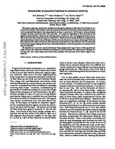
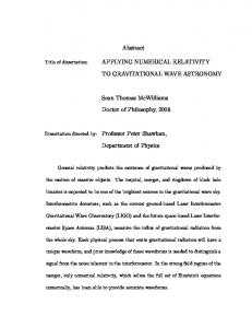
FIG. 1. Convergence results for the head-on collision of two BHs in D = 5 dimensions, for initial separation d/rS = 7 and d/rS = 6.47 (left and right panels respectively). Top panels refer to energy fluxes obtained respectively with SacraND and HDLean codes at different resolutions h. The corresponding convergence plots are shown in the bottom panels. Panel (a) indicates 4th order convergence for the simulation performed with the SacraND code. Panel (b) indicates 2nd order convergence for the simulations performed with the HD-Lean code.
fects diagnostics using gravitational radiation output. In order to estimate the numerical accuracy of both codes we have performed convergence tests using resolutions hc /rS = 1/72, hm /rS = 1/84 and hh /rS = 1/96 (for HD-Lean) and hc /rS = 1/50, hm /rS = 1/60 and hh /rS = 3/200 (for SacraND) near the BHs. A convergence analysis, summarized in Fig. 1 for the energy flux, shows second-order convergence for HDLean and fourth-order convergence for SacraND. The numerical error in the total radiated energy is estimated to be ∆Erad /Erad ∼ (0.7%, 1.3%)
the error due to the extraction at finite radii and the extrapolation to be about 5%. However, because our primary purpose here is to compare two different codes, we will compare their output at finite rex and therefore - since the quantities evaluated at finite rex are different in the two approaches - consider the 6 % total uncertainty estimate (from discretization and extrapolation) a conservative upper limit for the expected discrepancies between the two codes at a given extraction radius.
(3)
for HD-Lean and SacraND, respectively. In numerical time evolution codes, GW amplitudes are often measured at a finite “extraction” radius rex (but see Refs. [50, 51] for exceptions developed for the four-dimensional case). To compute physically relevant and unambiguous quantities, it is desirable to extrapolate these quantities to rex /rS → ∞: fluxes and GW amplitudes are measured at a sphere of arbitrarily large radius. The extrapolation procedure introduces an additional source of error. We estimate the radiated energy as it would be measured at rex /rS → ∞ by assuming an expansion of the form X rex j ∞ Aj /rex , (4) Erad =Erad + j=1,2,...
rex using the values Erad calculated at fixed extraction radii ∞ to estimate Erad and the associated error. We evaluate
C.
(Spurious) Radiation content in initial data
Due to the initial data construction, in which we assume the maximal slicing condition K = 0 and a finite initial distance between the BHs, the system contains a pulse of unphysical1 or spurious radiation, colloquially called “junk” radiation. This spurious radiation is typically emitted in a short burst after which the collision process proceeds normally. This is a well-known phenomenon in numerical relativity simulations of BH binaries in D = 4. Typically2 , starting the collision at
1
2
“Unphysical” in the sense that a binary BH at rest at infinite initial separation would not be accompanied by such pulse of radiation at any finite distance But not always, for example high energy collisions evolving conformally flat initial data are very challenging on account of the growing spurious radiation content at large Lorentz boosts [52, 53].
4 larger initial separations allows for the spurious radiation to leave the computational domain before interesting dynamics take place, therefore effectively eliminating its (undesirable) effect. The energy content in the “spurious” pulse grows as the initial separation between the two BHs decreases. This has been observed repeatedly in four-dimensional spacetimes [28, 54]. We observe a similar pattern in D = 5 spacetime dimensions. For simulations with initial separation d/rS = 3, 12 for example, the fraction of the total radiated energy in the initial pulse is estimated to be 3% and < 0.1% respectively. To avoid dealing with this spurious radiation we eliminate it from our analysis, by cutting it out of energy fluxes and waveforms; this is possible for large enough initial separations, but becomes increasingly difficult for small initial separation. D.
Energy flux and total radiated energy
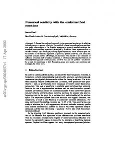
Results for the energy flux are shown in the left panel of Fig. 2. This is one of the main results of this work: both codes, using different dimensional reduction techniques and different diagnostic tools, yield the same result for the flux and total radiated energy within numerical errors. To avoid uncertainties with extrapolation methods, the energy flux shown in Fig. 2 is measured at a finite coordinate radius of rex /rS = 40. The flux and waveforms show a clear ringdown at late times. In particular, by fitting our numerical results to exponentially damped sinusoids, we estimate the l = 2 and l = 4 quasi-normal frequencies to be rS ωl=2 =0.95 − ı 0.26 , rS ωl=4 =2.12 − ı 0.36 .
(5a) (5b)
agreement between the two codes. Finally, the area of the final AH allows one to estimate also the radiated energy. These are in good agreement with the estimates obtained via wave extraction [17].
V.
HEAD-ON COLLISIONS IN D = 6
Previous results in the literature concerning detailed analysis of BH collisions were specialized to four and five spacetime dimensions. We now briefly describe results in D = 6, summarized in Fig. 3. A typical waveform is shown in the top left panel of Fig. 3. The GW signal, as measured by the gauge-invariant function Φ, displays the usual dominant quasi-normal ringdown. We estimate the ringdown parameters for the quadrupolar, l = 2, component to be given by rS ωl=2 = 1.14 − ı 0.30. This number compares very well against linearized calculations, which predict [55, 56] rS ωl=2 = 1.1369 − ı 0.3038. As we mentioned previously, the computation of the energy flux is performed at a finite extraction radius. The total integrated flux yields the energy radiated in GWs and is consequently also computed at a finite location. The physical total energy, computed at infinity, is estimated via extrapolation. These different quantities are shown in Fig. 3 for different BH initial separations. In the limit of infinite initial separation, the total radiated energy is Erad /M = (8.1 ± 0.4) × 10−4 .
(8)
This number is comparable to, but smaller than the corresponding value in D = 5 (see Eq. (7)), in agreement with the linearized point-particle calculations of Ref. [59].
We find good agreement with linearized predictions for the ringdown frequencies [55, 56] rS ωl=2 =0.9477 − ı 0.2561 , rS ωl=4 =2.1924 − ı 0.3293 .
(6a) (6b)
The right panel of Fig. 2 compares the total integrated energy for various initial separations using both codes. The behavior with initial separation d for five spacetime dimensions closely resembles the one found in fourdimensions [57, 58]: at very small initial separations the binary closely resembles a single distorted BH, and the radiation output is consequently very small. At large initial separations the radiation output asymptotes to a constant value, Erad /M = (9.0 ± 0.5) × 10−4
(7)
in agreement with Ref. [17]. There is a local maximum at finite initial separations, also reported in four-dimensional simulations in the point-particle limit [58]. We highlight again the close
VI.
CONCLUSIONS
Higher-dimensional spacetimes offer a vast and rich arena to test and understand the gravitational field equations. The demand to understand, at a quantitative level, complex dynamical processes was met by different, complex numerical codes and associated diagnostic tools. The main purpose of this work is to show that the current numerical infrastructure to handle BHs and BH-binaries in higher-dimensional spacetimes is solid and trustworthy. We have compared two different Numerical Relativity codes, HD-Lean [17, 23] and SacraND [18, 24] which use different “dimensional-reduction” techniques and different wave extraction methods. Our main result is that both codes yield the same answer, up to numerical errors which are under control. In addition, we determined the radiated energy in head-on collisions of six-dimensional black holes.
5
4e-04
3e-03 HD-LEAN SACRAND
HD-LEAN SACRAND
3e-04
E/M
dE / dt (M
-1/2
)
2e-03 2e-04
1e-03 1e-04
0e+00
0
25
50 (t - rex) / rS
75
0e+00
100
0
5
10
15
d/rs
(a) Energy fluxes
(b) Integrated fluxes
FIG. 2. Energy fluxes for head-on collisions of two BHs in D = 5 spacetime dimensions, obtained with HD-Lean (solid black line) and SacraND (red dashed line). The BHs start off at an initial coordinate separation d/rS = 6.47. The right panel shows the total integrated energy for different BH initial separations.
d / rS 8.6e-04
l=2
3
5
4
6
8
7
Erad / M
Φ,t
1e-02 1e-04
8.4e-04
8.2e-04
1e-06
Φ76 - Φ84 1.33 ( Φ84 - Φ92)
∆ Φ,t
0e+00
-2e-04
60
d / rS = 3.23 d / rS = 4.50 d / rS = 5.49 d / rS = 6.47 d / rS = 7.50
9.5e-04
Erad / M
2e-04
9.0e-04
8.5e-04
80
100
20
30
40
50
(t - rex) / rS
rex / rS
(a) Waveforms
(b) Energy
60
70
FIG. 3. Summary of results for head-on collisions in D = 6 spacetime dimensions. Left: Time derivative of the l = 2 multipole of the Kodama-Ishibashi gauge-invariant wavefunction Φ (top) and its convergence properties (bottom) computed with the HD-Lean code and measured at the extraction radius rex /rS = 40. The initial separation of the BHs has been d/rS = 6.47. The convergence factor Q2 = 1.33 indicates second order convergence. Right: Total radiated energy Erad /M emitted in the head-on collision of two BHs. The top panel shows the radiated energy, extrapolated to rex /rS → ∞ as a function of the initial separation d/rS . The bottom panel shows the radiated energy as a function of the extraction radius rex /rS for different initial separations.
ACKNOWLEDGMENTS
We thank the Yukawa Institute for Theoretical Physics at Kyoto University for hospitality during the YITP-T14-1 workshop on “Holographic vistas on Gravity and Strings.” H. W. acknowledges financial support provided under the ERC-2011-StG 279363–HiDGR ERC Starting
Grant. H.O. and V.C. acknowledge financial support provided under the European Union’s FP7 ERC Starting Grant “The dynamics of black holes: testing the limits of Einstein’s theory” grant agreement no. DyBHo– 256667. U.S. acknowledges support by FP7-PEOPLE2011-CIG Grant No. 293412 “CBHEO” and CESGAICTS Grant No. 249. M.Z. is supported by NSF
6 grants OCI-0832606, PHY-0969855, AST-1028087, and PHY-1229173. This research was supported in part by Perimeter Institute for Theoretical Physics. Research at Perimeter Institute is supported by the Government of Canada through Industry Canada and by the Province of Ontario through the Ministry of Economic Development & Innovation. This work was supported by the NRHEP 295189 FP7-PEOPLE-2011-IRSES Grant, the STFC GR Roller Grant No. ST/L000636/1, the Cos-
mos system, part of DiRAC, funded by STFC and BIS under Grant Nos. ST/K00333X/1 and ST/J005673/1, the NSF XSEDE Grant No. PHY-090003, and by project PTDC/FIS/116625/2010. Computations were performed on the “Baltasar Sete-Sois” cluster at IST, on “venus” cluster at YITP, on the COSMOS supercomputer in Cambridge, the CESGA Finis Terrae, SDSC Trestles and NICS Kraken clusters.
[1] R. Emparan and H. S. Reall, Living Rev.Rel. 11, 6 (2008), arXiv:0801.3471 [hep-th]. [2] R. Emparan, T. Harmark, V. Niarchos, N. A. Obers, and M. J. Rodriguez, JHEP 0710, 110 (2007), arXiv:0708.2181 [hep-th]. [3] T. Harmark, V. Niarchos, and N. A. Obers, Class.Quant.Grav. 24, R1 (2007), arXiv:hep-th/0701022 [hep-th]. [4] O. J. Dias, R. Monteiro, and J. E. Santos, JHEP 1108, 139 (2011), arXiv:1106.4554 [hep-th]. [5] O. J. C. Dias, G. S. Hartnett, and J. E. Santos, (2014), arXiv:1402.7047 [hep-th]. [6] V. Cardoso and O. J. Dias, Phys.Rev.Lett. 96, 181601 (2006), arXiv:hep-th/0602017 [hep-th]. [7] V. Cardoso, O. J. Dias, and L. Gualtieri, Int.J.Mod.Phys. D17, 505 (2008), arXiv:0705.2777 [hep-th]. [8] S. Bhattacharyya, V. E. Hubeny, S. Minwalla, and M. Rangamani, JHEP 0802, 045 (2008), arXiv:0712.2456 [hep-th]. [9] R. Emparan, T. Harmark, V. Niarchos, and N. A. Obers, JHEP 1003, 063 (2010), arXiv:0910.1601 [hep-th]. [10] F. Pretorius, Phys.Rev.Lett. 95, 121101 (2005), arXiv:gr-qc/0507014 [gr-qc]. [11] M. Campanelli, C. Lousto, P. Marronetti, and Y. Zlochower, Phys.Rev.Lett. 96, 111101 (2006), arXiv:gr-qc/0511048 [gr-qc]. [12] J. G. Baker, J. Centrella, D.-I. Choi, M. Koppitz, and J. van Meter, Phys.Rev.Lett. 96, 111102 (2006), arXiv:gr-qc/0511103 [gr-qc]. [13] V. Cardoso, L. Gualtieri, C. Herdeiro, and U. Sperhake, Living Reviews in Relativity (in preparation) (2014). [14] J. Aasi et al. (The LIGO Scientific Collaboration, the Virgo Collaboration, the NINJA-2 Collaboration), (2014), arXiv:1401.0939 [gr-qc]. [15] I. Hinder, A. Buonanno, M. Boyle, Z. B. Etienne, J. Healy, et al., Class.Quant.Grav. 31, 025012 (2014), arXiv:1307.5307 [gr-qc]. [16] L. Lehner and F. Pretorius, Phys.Rev.Lett. 105, 101102 (2010), arXiv:1006.5960 [hep-th]. [17] H. Witek, M. Zilhao, L. Gualtieri, V. Cardoso, C. Herdeiro, et al., Phys.Rev. D82, 104014 (2010), arXiv:1006.3081 [gr-qc]. [18] H. Okawa, K.-i. Nakao, and M. Shibata, Phys.Rev. D83, 121501 (2011), arXiv:1105.3331 [gr-qc]. [19] H. Witek, V. Cardoso, L. Gualtieri, C. Herdeiro, U. Sperhake, et al., Phys.Rev. D83, 044017 (2011), arXiv:1011.0742 [gr-qc].
[20] M. Shibata and H. Yoshino, Phys.Rev. D81, 104035 (2010), arXiv:1004.4970 [gr-qc]. [21] H. M. S. Yoshino and M. Shibata, Prog.Theor.Phys.Suppl. 189, 269 (2011). [22] V. Cardoso, L. Gualtieri, C. Herdeiro, U. Sperhake, P. M. Chesler, et al., Class.Quant.Grav. 29, 244001 (2012), arXiv:1201.5118 [hep-th]. [23] M. Zilhao, H. Witek, U. Sperhake, V. Cardoso, L. Gualtieri, et al., Phys.Rev. D81, 084052 (2010), arXiv:1001.2302 [gr-qc]. [24] H. Yoshino and M. Shibata, Phys.Rev. D80, 084025 (2009), arXiv:0907.2760 [gr-qc]. [25] M. Shibata and T. Nakamura, Phys.Rev. D52, 5428 (1995). [26] T. W. Baumgarte and S. L. Shapiro, Phys.Rev. D59, 024007 (1999), arXiv:gr-qc/9810065 [gr-qc]. [27] T. Yamamoto, M. Shibata, and K. Taniguchi, Phys.Rev. D78, 064054 (2008), arXiv:0806.4007 [gr-qc]. [28] U. Sperhake, Phys.Rev. D76, 104015 (2007), arXiv:gr-qc/0606079 [gr-qc]. [29] R. L. Arnowitt, S. Deser, and C. W. Misner, (1962), arXiv:gr-qc/0405109 [gr-qc]. [30] J. W. York, Jr., in Sources of Gravitational Radiation, edited by L. L. Smarr (1979) pp. 83–126. [31] M. Alcubierre, S. Brandt, B. Br¨ ugmann, D. Holz, E. Seidel, R. Takahashi, and J. Thornburg, Int. J. Mod. Phys. D 10, 273 (2001), gr-qc/9908012. [32] T. Goodale, G. Allen, G. Lanfermann, J. Mass´ o, T. Radke, E. Seidel, and J. Shalf (Springer, Berlin, 2003). [33] Cactus developers, “Cactus Computational Toolkit,” . [34] E. Schnetter, S. H. Hawley, and I. Hawke, Class.Quant.Grav. 21, 1465 (2004), arXiv:gr-qc/0310042 [gr-qc]. [35] J. Thornburg, Phys.Rev. D54, 4899 (1996), arXiv:gr-qc/9508014 [gr-qc]. [36] J. Thornburg, Class.Quant.Grav. 21, 743 (2004), arXiv:gr-qc/0306056 [gr-qc]. [37] R. P. Geroch, J.Math.Phys. 12, 918 (1971). [38] Y. Cho, Phys.Lett. 186, 38 (1987). [39] Y. Cho and D. Kim, J.Math.Phys. 30, 1570 (1989). [40] L. D. Landau and E. M. Lifshitz, The classical theory of fields, Vol. 2 (Butterworth-Heinemann, 1975). [41] V. Cardoso, O. J. Dias, and J. P. Lemos, Phys.Rev. D67, 064026 (2003), arXiv:hep-th/0212168 [hep-th]. [42] F. Tangherlini, Nuovo Cim. 27, 636 (1963).
7 [43] H. Kodama and A. Ishibashi, Prog.Theor.Phys. 110, 701 (2003), arXiv:hep-th/0305147 [hep-th]. [44] A. Ishibashi and H. Kodama, Prog.Theor.Phys.Suppl. 189, 165 (2011), arXiv:1103.6148 [hep-th]. [45] T. Regge and J. A. Wheeler, Phys.Rev. 108, 1063 (1957). [46] F. J. Zerilli, Phys.Rev.Lett. 24, 737 (1970). [47] F. J. Zerilli, Phys. Rev. D 2, 2141 (1970). [48] V. Moncrief, Ann. Phys. 88, 323 (1974). [49] E. Berti, M. Cavaglia, and L. Gualtieri, Phys.Rev. D69, 124011 (2004), arXiv:hep-th/0309203 [hep-th]. [50] C. Reisswig, N. Bishop, D. Pollney, and B. Szilagyi, Phys.Rev.Lett. 103, 221101 (2009), arXiv:0907.2637 [gr-qc]. [51] M. Babiuc, B. Szilagyi, J. Winicour, and Y. Zlochower, Phys. Rev. D 84, 044057 (2011), arXiv:1011.4223 [grqc]. [52] U. Sperhake, V. Cardoso, F. Pretorius, E. Berti, and J. A. Gonzalez, Phys.Rev.Lett. 101, 161101 (2008),
arXiv:0806.1738 [gr-qc]. [53] U. Sperhake, E. Berti, V. Cardoso, and F. Pretorius, Phys. Rev. Lett. 111, 041101 (2013), arXiv:1211.6114 [gr-qc]. [54] C. Lousto and R. H. Price, Phys.Rev. D69, 087503 (2004), arXiv:gr-qc/0401045 [gr-qc]. [55] H. Yoshino, T. Shiromizu, and M. Shibata, Phys.Rev. D72, 084020 (2005), arXiv:gr-qc/0508063 [gr-qc]. [56] E. Berti, V. Cardoso, and A. O. Starinets, Class.Quant.Grav. 26, 163001 (2009), arXiv:0905.2975 [gr-qc]. [57] P. Anninos, D. Hobill, E. Seidel, L. Smarr, and W.-M. Suen, Phys.Rev.Lett. 71, 2851 (1993), arXiv:gr-qc/9309016 [gr-qc]. [58] C. O. Lousto and R. H. Price, Phys.Rev. D55, 2124 (1997), arXiv:gr-qc/9609012 [gr-qc]. [59] E. Berti, V. Cardoso, and B. Kipapa, Phys.Rev. D83, 084018 (2011), arXiv:1010.3874 [gr-qc].