Higher-order interactions stabilize dynamics in competitive network ...

Higher-order interactions stabilize dynamics in competitive network models Jacopo Grilli1 , György Barabás1 , Matthew J. Michalska-Smith1 and Stefano Allesina1,2,3 1 Ecology

& Evolution, University of Chicago, 1101 E. 57th Chicago, IL 60637, USA 2 Computation Institute, University of Chicago 3 Northwestern Institute on Complex Systems, Northwestern University Nature (2017) 548:210-213 Abstract

Ecologists have long sought a way to explain how the staggering biodiversity observed in nature is maintained. On the one hand, simple models of interacting competitors cannot produce the stable persistence of very large ecological communities 1–5 ; on the other hand, neutral models 6–9 , in which species do not interact and diversity is maintained by immigration and speciation, yield unrealistically small fluctuations in population abundance 10 , and a strong positive correlation between a species’ abundance and its age 11 , contrary to empirical evidence. Models allowing for the robust persistence of large communities of interacting competitors are lacking. Here we show that very rich communities could persist thanks to the stabilizing role of higherorder interactions 12,13 , in which the presence of a species influences the interaction between other species. The existence of higher-order interactions has been debated in ecology for decades 14–16 , but their role in shaping ecological communities is still understudied 5 . Our results show that higher-order interactions can have dramatic effects on the dynamics of ecological systems, producing models in which coexistence is robust to the perturbation of both population abundances and parameter values. Introducing higher-order interactions has strong effects on models of closed ecological communities, as well as simulations of open communities in which new species are constantly introduced. Notably, in our framework higher-order interactions are completely defined by pairwise interactions, easing empirical parameterization and validation of our models.

Here we study deterministic models describing communities in which the number of individuals is large and the system is isolated (e.g., bacterial strain competition in laboratory conditions 17 ); in the Supplementary Information (S4) we examine the case in which the dynamics are stochastic, which best describe communities in which the number of individuals is finite. Finally, we allow new species to be introduced at a given rate, allowing for a comparison with neutral models (Supplementary Information S5). While our results hold for a wide class of systems, to exemplify our findings we consider the dynamics of a forest in which there is a fixed, large number of trees, so that we can simply track xi (t), the proportion of trees of species i at time t, with ∑i xi (t) = 1. At each step, a randomly selected 1

Higher-order interactions stabilize competitive dynamics

Nature (2017) 548:210-213

Page 2

tree dies, opening a gap in the canopy (i.e., we initially assume identical per capita death rates for all species). This event ignites competition among seedlings to fill the gap. Suppose that all individuals produce the same number of seedlings, and that we pick two seedlings at random, with the winner of the competition filling the gap (Fig. S1). The matrix H encodes the dominance relationships among the species: Hi j is the probability that the first seedling, belonging to species i, wins against the second seedling, belonging to species j. Clearly, Hii = 1/2 for all i, and Hi j + H ji = 1 for all i and j. If all Hi j = 1/2, we recover a neutral model. At the other extreme lies a model in which each pair (Hi j , H ji ) is either (1, 0) or (0, 1) (i.e., species i always wins or always loses against j), in which case H is called a “tournament matrix” 18 . A number of results have been derived for this case 19 , showing that coexistence is possible when species form “intransitive cycles” of competitive dominance, such as in the rock-paper-scissors game 20 . Here we extend these previous findings 19 to the most general case in which interactions range from neutral to complete dominance. We can approximate the dynamics of the n species as dxi (t) = xi (t)2 ∑ Hi j x j (t) − xi (t), dt j

(1)

where −xi (t) models the death process, and xi (t)2Hi j x j (t) is the probability of picking two seedlings of species i and j, with i winning the competition. The factor 2 arises from the fact that we could pick i first and j second, or vice versa, with the same outcome. Simple manipulations (Supplementary Information S1) show that these equations are equivalent to the system dxi (t) = xi (t) ∑ Pi j x j (t), (2) dt j which is the celebrated replicator equation 21,22 for a zero-sum, symmetric matrix game with two players and payoffs encoded in the skew-symmetric matrix P = H − Ht . This equation is at the core of evolutionary game theory, with applications spanning multiple fields 23,24 . Thanks to this equivalence, we are able to characterize the dynamics. Unless specified, we assume H to be of full rank, i.e., all of its eigenvalues are nonzero. We show in the Supplementary Information that violations of this assumption are unbiological, amounting to degenerate cases in which slightly altering the parameters dramatically changes the outcome. Suppose that we start with n species and initial conditions xi (0) > 0, and that we let the dynamics unfold. Once the transient dynamics have elapsed, we find k ≤ n coexisting species, with k being odd. The n − k species that go extinct do so irrespective of initial conditions, and the k coexisting species cycle neutrally around a unique equilibrium point x∗ (Fig. 1, Supplementary Information S1). How large is k when we build the matrix H at random? When drawing Hi j (with i < j) from the uniform distribution U [0, 1] and setting the corresponding H ji = 1 − Hi j , we find that the probability of having k species coexisting when starting with n, p(k|n) = 0 when k is even, and p(k|n) = nk 21−n when k is odd 25 (Fig. S2). This matches what found for tournament games 18,19,26 , in which dominance is complete: we expect half of the initial species to coexist, irrespective of the choice of n; moreover, monodominance is extremely rare, and about as rare as the coexistence of all species. Thus, this theory generates high biodiversity without the need to fine-tune parameters. This model can generate any species-abundance distribution: for any choice of x∗ , we can build infinitely many matrices H such that Eqs. 1 and 2 have x∗ as an equilibrium (Supplementary Information S1). Note that this is true irrespective of the fact that x∗ contains an even or odd number of


Nature (2017) 548:210-213

Page 3

a)

b)

c)

d)

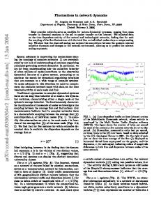
Figure 1: Sampling two seedlings: cycles. Dynamics of a forest where two randomly sampled seedlings compete to fill the gap in the canopy opened by the death of a tree. Seedlings of species i have probability Hi j of winning against those of species j (shade of the arrowheads; Hi j + H ji = 1). a) When starting with n species, n − k species go extinct, and k coexist. Given a matrix H, the identity of the species coexisting or going extinct is the same irrespective of initial conditions. The k species that coexist cycle neutrally around a single equilibrium point. b) The same is found when dominance is complete, such as in the rock-paper-scissors game 19 . c) For any possible species-abundance distribution x∗ , we can build a matrix H such that the species coexist and x∗ is an equilibrium of Eq. 1 (Supplementary Information S1). This is true even when x∗ contains an even number of species— though this case is not robust to small changes in parameters (Supplementary Information, Fig. S4). d) The same holds for any number of species in the system.


Nature (2017) 548:210-213

Page 4

species (Fig. 1)—but the case in which an even number of species coexist is degenerate: the system has infinitely many neutrally stable equilibria, and a slight change of H would result in the extinction of at least one species (Supplementary Information, Fig. S4). In summary, the model in Eq. 1 can lead to arbitrarily many species coexisting even when competitive abilities are drawn at random; moreover, it can generate any possible species-abundance distribution. While the neutral cycling around equilibrium is problematic (such cycles are not observed in nature, and would lead to monodominance in a noisy, stochastic world, Supplementary Information S4), the main issue with this model is that it is highly unrobust: any deviation from perfectly identical death rates and fecundities for all species destabilizes dynamics, leading to monodominance (Supplementary Information, Fig. S4). Following recent mathematical results 27 , we explore a possible solution to this problem. So far, we have taken exactly two seedlings, competing with each other to fill the gap in the canopy. In nature, we would observe a much richer seedbank, potentially leading to the competition among many seedlings. We therefore study a model in which we take three seedlings at random, compete the first with the second, and the winner with the third. The deterministic approximation of this model reads ! dxi (t) (3) = xi (t) ∑(2Hi j Hik + Hi j H jk + Hik Hk j )x j (t)xk (t) − 1 , dt j,k where Hi j Hik is the probability that i beats both j and k, Hi j H jk that j beats k, but ultimately is beaten by i, and Hik Hk j that first k beats j, and then i beats k. Surprisingly, this small modification leads to a major change in the dynamics: though the equilibrium point is unchanged, it is now globally stable (Fig. 2 and Supplementary Information S1). Increasing the number of seedlings that compete to fill each gap simply accelerates the dynamics, speeding up convergence to the equilibrium (Fig. S3). While the model in which we sample two seedlings yields the replicator equation for a two-player, symmetric matrix game, Eq. 3 is equivalent to the replicator equation for a three-player game (Supplementary Information S1): dxi (t) = xi (t) ∑ Pi jk x j (t)xk (t), (4) dt j,k where P is a 3-index tensor encoding the payoff of player 1 playing strategy i when player 2 plays j and player 3 plays k. The payoffs can be calculated from the matrix H: Pi jk = 2Hi j Hik − H ji H jk − Hki Hk j (where the first term includes the probability of i winning against both j and k, and the remaining two terms the probability that either j or k dominate). This latter formulation makes it clear that the stabilizing effect is due to higher-order interactions 5,12 : suppose the matrix H is constructed as in a rock-paper-scissors game; then the presence of the rock-plant can reverse the outcome of the competition between the paper- and the scissorsplant. In our model, higher-order interactions do not alter equilibrium values, but have a dramatic stabilizing effect, leading to globally stable fixed points instead of neutral cycles. Including fourth- or higher-order terms simply accelerates the convergence to equilibrium. As such, as long as there is a chance of competing more than two seedlings at a time, dynamics will converge. Most importantly, results are qualitatively robust to the perturbations of the death rates and fecundities of the competitors (Supplementary Information, Fig. S4). One formidable challenge of estimating higher-order interactions empirically is that for n species n we have 2 = n(n − 1)/2 pairs of interactions, but the number of triplets is much higher ( n3 =


Nature (2017) 548:210-213

Page 5

a)

b)

c)

d)

Figure 2: Sampling three seedlings: stability. When we sample three seedlings at a time instead of two, and we compete the first with the second and the winner with the third, the equilibrium point is unchanged, but is now globally attractive. The four cases correspond to those in Fig. 1.


Nature (2017) 548:210-213

Page 6

n(n − 1)(n − 2)/6)—requiring many experiments. Instead of introducing new coefficients, here we have chosen the most “natural” and conservative parameterization: higher-order interactions are fully determined by pairwise interactions, as shown by the fact that we can write all models in terms of the pairwise relationships encoded in H. This makes the models empirically testable by, for example, competing bacteria in laboratory conditions 17 . We have shown the equivalence of models in which competition happens in a sequence of bouts (Eq. 3) with models in which interactions are simultaneous and involve more than two species at a time (Eq. 4). Because of a separation of timescales (the filling of a gap is fast, compared to the lifespan of trees), the two types of models have the same deterministic form, blurring the traditionally-held distinction between so-called interaction chains and “proper” higher-order interactions 5,28 . Our results may have important implications for a variety of ecological systems; for example, in models in which reproduction is not instantaneously coupled with consumption, an animal could consume a resource, but be consumed before reproduction—yielding the same mechanism that stabilizes our competitive communities when we sample three seedlings at a time. Similarly, the stabilizing role of higher-order interactions in random replicator equations has been recently proposed 29 , and our analytical results shed light on these findings. Moving from deterministic to stochastic models, we find that the presence of higher-order interactions, which make equilibrium points attractive, dramatically increase 30 time to extinction in isolated systems, allowing for the prolonged coexistence of species (Supplementary Information S4). When we open the system to the introduction of new species (Supplementary Information S5), we recover many of the main results of neutral theory, but remove the artifactual relationship between a species age and its abundance—one of the main drawbacks of neutral models 11 . Our results strengthen the theory of coexistence in zero-sum competitive networks in several ways. First, we have widespread coexistence without having to invoke either of two extreme cases: perfect ecological equivalence (neutral model) or complete dominance (coexistence through intransitive competition). In nature, the outcome of competition could be mediated by a number of factors (e.g., soil chemistry, presence of consumers), so that competitive dominance could range from neutral to complete. Second, many species coexist even when we draw parameters at random, meaning that the results are highly robust. Third, in this formulation, the notion of intransitivity, which is central to coexistence in competitive networks in which dominance is complete 19 , is no longer necessary for coexistence (Supplementary Information S3). Fourth, the artifact of neutral cycling is due to the choice of only two competitors per bout—a choice dictated by mathematical convenience rather than by empirical evidence. Including more biological realism in the form of multiple competing species removes the artifact, leading to dynamics that are stable against perturbations of species abundances and robust against changing model parameters.

Acknowledgements Thanks to J. Aljadeff, F. Brandl, J.A. Capitán, J-F. Laslier, J.M. Levine, C.A. Marcelo Serván, and E. Sander for comments and discussions. E. Leigh and four anonymous referees provided constructive feedback. J.G. supported by the Human Frontier Science Program; S.A. and G.B by NSF DEB1148867; M.J. M-S. by US Department of Education grant P200A150101.


Nature (2017) 548:210-213

Page 7

References [1] May, R. M. Will a large complex system be stable? Nature 238, 413–414 (1972). [2] Clark, J. S. et al. High-dimensional coexistence based on individual variation: a synthesis of evidence. Ecological Monographs 80, 569–608 (2010). [3] Barabás, G., J. Michalska-Smith, M. & Allesina, S. The effect of intra-and interspecific competition on coexistence in multispecies communities. The American Naturalist 188, E1–E12 (2016). [4] D’Andrea, R. & Ostling, A. Challenges in linking trait patterns to niche differentiation. Oikos 125, 1369–1385 (2016). [5] Levine, J., Bascompte, J., Adler, P. & Allesina, S. Beyond pairwise coexistence: biodiversity maintenance in complex ecological communities. Nature (in press) (2017). [6] Hubbell, S. P. The unified neutral theory of biodiversity and biogeography, vol. 32 (Princeton University Press, 2001). [7] Volkov, I., Banavar, J. R., Hubbell, S. P. & Maritan, A. Neutral theory and relative species abundance in ecology. Nature 424, 1035–1037 (2003). [8] Alonso, D., Etienne, R. S. & McKane, A. J. The merits of neutral theory. Trends in Ecology & Evolution 21, 451–457 (2006). [9] Azaele, S. et al. Statistical mechanics of ecological systems: Neutral theory and beyond. Reviews of Modern Physics 88, 035003 (2016). [10] Chisholm, R. A. et al. Temporal variability of forest communities: empirical estimates of population change in 4000 tree species. Ecology Letters 17, 855–865 (2014). [11] Chisholm, R. A. & O’Dwyer, J. P. Species ages in neutral biodiversity models. Theoretical Population Biology 93, 85–94 (2014). [12] Billick, I. & Case, T. J. Higher order interactions in ecological communities: what are they and how can they be detected? Ecology 75, 1529–1543 (1994). [13] Werner, E. E. & Peacor, S. D. A review of trait-mediated indirect interactions in ecological communities. Ecology 84, 1083–1100 (2003). [14] Case, T. J. & Bender, E. A. Testing for higher order interactions. The American Naturalist 118, 920–929 (1981). [15] Abrams, P. A. Arguments in favor of higher order interactions. The American Naturalist 121, 887–891 (1983). [16] Kareiva, P. Special feature: Higher Order Interactions as a Foil to Reductionist Ecology. Ecology 75, 1527–1528 (1994).


Nature (2017) 548:210-213

Page 8

[17] Friedman, J., Higgins, L. M. & Gore, J. Community structure follows simple assembly rules in microbial microcosms. Nature Ecology & Evolution 1, 0109 (2017). [18] Fisher, D. C. & Ryan, J. Optimal strategies for a generalized “scissors, paper, and stone” game. American Mathematical Monthly 99, 935–942 (1992). [19] Allesina, S. & Levine, J. M. A competitive network theory of species diversity. Proceedings of the National Academy of Sciences USA 108, 5638–5642 (2011). [20] Kerr, B., Riley, M. A., Feldman, M. W. & Bohannan, B. J. Local dispersal promotes biodiversity in a real-life game of rock–paper–scissors. Nature 418, 171–174 (2002). [21] Taylor, P. D. & Jonker, L. B. Evolutionary stable strategies and game dynamics. Mathematical Biosciences 40, 145–156 (1978). [22] Hofbauer, J., Schuster, P. & Sigmund, K. A note on evolutionary stable strategies and game dynamics. Journal of Theoretical Biology 81, 609–612 (1979). [23] Hofbauer, J. & Sigmund, K. Evolutionary game dynamics. Bulletin of the American Mathematical Society 40, 479–519 (2003). [24] Nowak, M. A. & Sigmund, K. Evolutionary dynamics of biological games. Science 303, 793– 799 (2004). [25] Brandl, F. The distribution of optimal strategies in symmetric zero-sum games. arXiv preprint arXiv:1611.06845 (2016). [26] Fisher, D. C. & Reeves, R. B. Optimal strategies for random tournament games. Linear Algebra and its Applications 217, 83–85 (1995). [27] Laslier, B. & Laslier, J.-F. Reinforcement learning from comparisons: Three alternatives is enough, two is not. arXiv preprint arXiv:1301.5734 (2013). [28] Wootton, J. T. Indirect effects and habitat use in an intertidal community: interaction chains and interaction modifications. The American Naturalist 71–89 (1993). [29] Bairey, E., Kelsic, E. D. & Kishony, R. High-order species interactions shape ecosystem diversity. Nature Communications 7 (2016). [30] Reichenbach, T., Mobilia, M. & Frey, E. Coexistence versus extinction in the stochastic cyclic Lotka-Volterra model. Physical Review E 74, 051907 (2006).


Nature (2017) 548:210-213

Page 9

Methods To exemplify the role of higher-order interactions in shaping ecological dynamics, we consider a model of a forest in which whenever a tree dies, a certain number of seedlings compete to fill the gap (m) in the canopy (Fig. S1). We start by writing the microscopic rate Wi j at which species j loses an individual (η j → η j − 1), while species i gains an individual (ηi → ηi + 1). The index m specifies that we consider the case in which m seedlings at a time compete to fill in the gap. When there are many individuals we can track proportions (xi (t) = ηi (t)/ ∑ j η j (t)), and setting m = 2, we can write this rate as: (2)

Wi j = d j x j

fi xi ∑l fl xl

f k xk

∑ 2Hik ∑l fl xl

(5)

k

in which fi and di are the fecundity and death rate of trees belonging to species i. Using the notation F(x) = ∑l fl xl , the term fi xi / ∑l fl xl = fi xi /F(x) is the proportion of seeds in the seedbank belonging to species i. Finally, the matrix H encodes the probability of winning for every pair of species, so that Hik is the probability of seedling of species i beating those of species k, and the factor 2 arises from (2) the fact that we could sample i first and k second, or vice versa. Then, the term Wi j can be interpreted as the rate at which a) a tree of species j dies, and b) two seedlings of species i and k are sampled, with i filling the gap. Because the identity of k does not matter, we sum over all possible choices. When the number of trees is sufficiently large, we can neglect stochasticity and write: ! dxi D(x) (2) (2) fi Hik fk xk − di (6) = ∑ Wi j −W ji = xi dt F(x)2 ∑ j k

where we have introduced D(x) = ∑l dl xl . In Supplementary Information S4 we present stochastic simulations that show strong agreement with the predictions of this deterministic approximation. We can derive equations like Eq. 6 for any choice of m. We write: (m)

Wi j

(m)

= d j x j qi

(7)

(m)

where qi is the probability that a seedling of species i wins when competing against m − 1 other (m) seedlings. We build qi recursively:  f i xi (1)   qi =  F(x)  (8) ...   fi xi f k xk  (m) (m−1) (m−1)  + qi qi = ∑ Hik qk ∑k Hik F(x) k F(x)

f i xi (m−1) is the probability that i wins against the winner ∑ Hik qk F(x) k fk xk (m−1) of the competition of involving the first m − 1 seedlings, while qi is the probability ∑k Hik F(x) that i is the winner of the competition among the first m − 1 seedlings, and beats the last seedling. (m) Consistently with the fact that these are probabilities, ∑i qi = 1 for any m. In this way, we can for (2) example recover the rate Wi j we have introduced above: which has a simple interpretation:


(2)

(2)

Wi j = d j x j qi = d j x j

Nature (2017) 548:210-213

f i xi f k xk (1) (1) Hik qk + qi ∑ Hik ∑ F(x) k F(x) k

!

= d jx j

f i xi fk xk 2Hik ∑ F(x) k F(x)

Page 10

(9)

In general, the dynamics when considering m seedlings become: dxi (m) (m) (m) = D(x)qi − di xi . = ∑ Wi j −W ji dt j

(10)

Using this formulation, we write the system of equations describing the model in which three (3) seedlings are sampled. We calculate qi : (3)

f i xi fk xk (2) (2) Hik qk + qi ∑ Hik ∑ F(x) k F(x) k f jx j f jx j f i xi fk xk f i xi f k xk = 2Hi j H jk + 2Hi j Hik ∑ ∑ F(x) j,k F(x) F(x) F(x) j,k F(x) F(x) f j x j f k xk f i xi = 2Hi j H jk + 2Hi j Hik ∑ F(x) j,k F(x) F(x) f j x j f k xk f i xi Hi j H jk + Hik Hk j + 2Hi j Hik = F(x) ∑ F(x) F(x) j,k

qi =

yielding the system of equations

dxi D(x) (3) (3) fi ∑ 2Hi j Hik + Hi j H jk + Hik Hk j f j x j fk xk − di = ∑ Wi j −W ji = xi 3 dt F(x) j j,k

!

(11)

Having derived this general case, we dedicate Supplementary Information S1 to the study of the simplified model we have introduced in the main text, in which fi = di = 1 for all i. It is easy to derive a number of results for this simplified formulation, including the existence and uniqueness of the coexistence equilibrium, the stability properties of such equilibrium when sampling two or more than two seedlings, the expected number of coexisting species when H is random, and the construction of an algorithm that takes as input a desired species-abundance distribution x∗ , and produces infinitely many H such that x∗ is an equilibrium of the system. In Supplementary Information S2, we return to the more general case introduced above to test the robustness of our findings when we relax the strong constraint of identical physiological rates for all species. Supplementary Information S3 is dedicated to the discussion of intransitivity. Finally, Supplementary Information S4 and S5 extend these models to situations in which the number of individuals is finite, and therefore demographic stochasticity becomes important. We first consider the case of an isolated ecological community (S4), and then open the community to the introduction of new species by immigration or speciation (S5), allowing for a direct contrast with neutral models.

Higher-order interactions stabilize dynamics in competitive network models Supplementary Information Jacopo Grilli1 , György Barabás1 , Matthew J. Michalska-Smith1 and Stefano Allesina1,2,3 1 Department

of Ecology & Evolution, University of Chicago, 1101 E. 57th Chicago, IL 60637, USA 2 Computation Institute, University of Chicago 3 Northwestern Institute on Complex Systems, Northwestern University Nature (2017) 548:210-213

S1

Identical physiological rates

In the Methods we have shown that, when considering systems with a large number of individuals, our model (depicted in Fig. S1) can be written as a system of differential equations: dxi (m) (m) (m) = ∑ Wi j −W ji = D(x)qi − di xi , dt j

(S1) (m)

where m is the number of seedlings that compete for filling each gap, Wi j

(m) qi

viduals of species j are replaced by those of species i, and the function  f i xi (1)   qi =   F(x)  ...   f i xi fk xk  (m) (m−1) (m−1)  + qi qi = ∑k Hik qk ∑k Hik F(x) F(x)

is the rate at which indican be built recursively:

(S2)

.

For the cases of two seedlings competing, the equations describing the dynamics become: ! dxi D(x) (2) (2) = ∑ Wi j −W ji = xi fi Hik fk xk − di , dt F(x)2 ∑ j k

(S3)

and those describing the case in which we sample three seedlings become:

dxi D(x) (3) (3) = ∑ Wi j −W ji = xi fi ∑ 2Hi j Hik + Hi j H jk + Hik Hk j f j x j fk xk − di 3 dt F(x) j j,k 11

!

.

(S4)


Nature (2017) 548:210-213

Page 12

Processes a) death

Dynamics a) a tree dies

b) fecundities

b) seedlings are pooled, m are sampled and compete in sequence m=3

fi

c) competition

c) the winner fills the gap

Hij

Hji

Figure S1: Illustration of the model, Left: the dynamics are controlled by the following parameters: (a)

di , the death rate of species i; (b) fi , the fecundity of species i; and (c) the matrix H, detailing the probability that seedling from one species win against seedling of other species when competing to fill a gap. Right: a) whenever a tree dies, we pool the seedlings, and select m to compete (b), with the winner filling the gap (c).

In this section, we study these models when we make the simplifying assumption of equal physiological rates (di = fi = 1) for all species.

S1.1 Sampling two seedlings When setting all fi = di = 1 in Eq. S3, we obtain Eq. 1 of the main text: dxi = xi 2 ∑ Hi j x j − xi dt j

(S5)

We want to show that this is equivalent to the replicator equation, Eq. 2 of the main text: dxi = xi ∑ Pi j x j dt j where P = H − Ht . This is easy to show:

(S6)


xi

!

∑ 2Hi j x j − 1 j

Nature (2017) 548:210-213

Page 13

= xi ∑(2Hi j x j − x j ) j

= xi ∑(Hi j x j + (1 − H ji )x j − x j ) j

= xi ∑(Hi j − H ji )x j j

= xi ∑ Pi j x j j

If x∗ is an equilibrium such that xi ∗ > 0 for all i, then Px∗ = 0, meaning that x∗ is an eigenvector of P, corresponding to a zero eigenvalue. The formulation in terms of P is also useful to connect to important results in game theory: P is the payoff matrix for a two-player, zero-sum symmetric matrix game. Then, when H is random, the game admits only one optimal strategy 1,2 , which in general is a mixed strategy composed of k pure strategies, with k odd. The optimal strategy corresponds to the equilibrium x∗ . This means that, starting the dynamics with n species and any positive initial conditions, the same n − k species will go extinct, and the same k species will coexist. Though we believe that mild deviations from zero-sum (for example, cases in which the number of individuals is fixed on average) would not change qualitatively our results, we maintain this assumption out of mathematical convenience, and because it allows us to connect directly with the afore-mentioned results in game theory. S1.1.1 Neutral cycling Next, we want to show that the species that coexist cycle neutrally around the single equilibrium point. To do so, we construct a Lyapunov function for the system and show that we can find a constant of motion for system—meaning that trajectories will follow closed orbits. Suppose xi∗ > 0 is the equilibrium of Eq. 1 of the main text. We write the function V (x) = − ∑ xi∗ log i

xi . xi∗

(S7)

Because of Gibbs’ inequality, V (x) ≥ 0 for any 0 < xi < 1 and it is equal to zero only if xi = xi∗ for all i. Note also that at equilibrium 2 ∑ j Hi j x∗j = 1. We write ∂V dxi dV =∑ dt ∂ xi dt i x∗ dxi = −∑ i i xi dt

= −2 ∑ xi∗ Hi j x j + ∑ xi∗ i, j

= −2 ∑ i, j

i ∗ xi Hi j x j + 1


= ∑ −2 ∑ i

j

Hi j xi∗

!

i

Page 14

xj +1

= ∑ −2 ∑ j

Nature (2017) 548:210-213

(1 − H ji )xi∗

!

xj +1 !

= ∑ −2 ∑ xi∗ + 2 ∑ H ji xi∗ x j + 1 j

i

i

= ∑(−2 + 1)x j + 1 j

= −∑xj +1 j

= 0. Thus, we have found a constant of motion, meaning that the system will follow closed orbits. Hence, unless we start the system precisely at x∗ , the abundances will cycle neutrally around the equilibrium. S1.1.2

Number of coexisting species for random interactions

Now we ask how many species will coexist when we draw the matrix H at random. We build random matrices in two ways. First, we set each pair (Hi j , H ji ) to (1, 0) with probability 1/2, and to (0, 1) with probability 1/2; the diagonal elements are all set to 1/2. In this model, dominance is complete, and the matrix H describes a tournament—a complete directed graph in which for each pair of species, an arrow connects the winner to the loser. Second, for each pair (Hi j , H ji ) (i 6= j) we sample a random number z from the uniform distribution U [0, 1], and set the values to (1 − z, z); again, Hii = 1/2 for all i. Thus H encodes a generalization of tournament graphs, called hypertournaments 3 . We set n = 50, and build 10,000 matrices of each kind. The number of coexisting species k can be found solving the corresponding linear program, as done by Allesina & Levine 4 . Finally, we tally the number of coexisting species to estimate p(k|n). The results, reported in Fig. S2 show that both settings result in the same histogram: p(k|n) = 0 when k is even, and p(k|n) = nk 21−n when k is odd, as predicted both for random tournaments 4,5 and hypertournaments 2 . S1.1.3

Building H given x∗

Finally, we provide an elementary argument for why only an odd number of species coexist at equilibrium, unless we fine-tune parameters. The argument allows us to build an algorithm that accepts as input a desired species-abundance distribution x∗ , and produces infinitely many matrices H such that x∗ is an equilibrium of Eq. 1, or Eq. 2 of the main text. As we stated above, if all xi ∗ > 0 is an equilibrium, then x∗ is an eigenvector of P corresponding to a zero eigenvalue. A matrix with one or more zero eigenvalues is rank-deficient. Fisher & Ryan 6 proved that, if the n × n matrix H represents a tournament, then P has rank n when n is even, and rank n − 1 when n is odd. Therefore, the matrix P will have an eigenvalue of zero only if n is odd—when the matrix H is a tournament matrix, only an odd number of species can coexist.


Nature (2017) 548:210-213

Page 15

Figure S2: Number of coexisting species with random competition. Number of coexisting species k in a random tournament (red) or hypertournament (blue) when the number of initial species is n = 50. Bars: proportion of random (hyper)tournaments leading to the coexisting of k species (out of 10,000 simulations). Crosses: analytical expectation (p(k|n) = 0 when k is even, nk 21−n when k is odd).


Nature (2017) 548:210-213

Page 16

When we build the matrix H at random by sampling the coefficients from a uniform distribution, we have that the matrix has full rank (i.e., the set of rank-deficient matrices has measure zero). For these matrices then, the same result found for tournaments holds 2 . Clearly, one could build rank-deficient matrices—only, it is impossible to find this result at random when sampling the coefficients from a continuous distribution. In the next paragraphs, we show having a rank-deficient H automatically introduces a neutral manifold of infinitely many equilibria, and that this case is unrobust: small perturbations of the coefficients will lead to an odd number of species coexisting. Armed with these results, we can build an algorithm that takes a desired relative species abundance ∗ x , and builds a matrix H such that Eq. 1 and Eq. 2 have x∗ as an equilibrium. In fact, we show that one can construct infinitely many matrices of this kind. The algorithm also makes apparent the implicit assumptions we are making when we want an even number of species to coexist indefinitely. The strategy is to build a matrix of eigenvectors U for the skew-symmetric matrix P, and the corresponding diagonal matrix of eigenvalues Λ . Then, P = UΛ Λ U−1 . Finally, we have that Hi j = (Pi j + 1)/2. The first case we examine is that of an odd number of species, n. We set the real vector r1 = x∗ , and draw n − 1 random, real-valued vectors, r2 , . . . , rn . We modify the vectors r2 , . . . , rn to make them orthogonal to r1 and each other. Writing U j as the jth column of U,√ we set: U1 = r1 = x∗ , U2 = r2 + i r3 , U3 = r2 − i r3 , U4 = r4 + i r5 , U5 = r4 − i r5 , etc. (note that i = −1). Finally, we need to set the eigenvalues. We choose Λ1,1 = 0, and we set the remaining eigenvalues in pairs: we draw a random number z, and set Λ2,2 = i z, Λ3,3 = −i z; draw a second random number to determine Λ4,4 and Λ5,5 , etc. Once we have chosen the eigenvalues and eigenvectors, we compute P, and, if needed, normalize the matrix such that min Pi j ≥ −1 and max Pi j ≤ 1 (dividing all elements by a constant simply re-scales the spectrum). Note that we have complete freedom in choosing all the eigenvalues and eigenvectors, besides the first. Hence, we can produce infinitely many matrices P that have x∗ as an eigenvector associated with a zero eigenvalue, and therefore we can produce infinitely many matrices H. If x∗ contains an even number of species, we proceed in almost the same way, but we now need two eigenvalues to be 0 (because the matrix P needs to be skew-symmetric, all the eigenvalues must have real part 0, and conjugate imaginary parts), and two eigenvectors to be real. Therefore, we construct the matrix U as: U1 = r1 = x∗ , U2 = r2 , U3 = r3 + i r4 , U4 = r3 − i r4 , U5 = r5 + i r6 , U6 = r5 − i r6 , etc. We set Λ1,1 = Λ2,2 = 0, and the remaining eigenvalues at random, as done for n odd. Again, we can build infinitely many P and therefore H. This means that in order to have an equilibrium containing an even number of species, we need to set two eigenvalues to zero: the matrix has rank n − 2, so that the rows/columns of P are no longer linearly independent. This is a very fragile situation, as small modifications of the coefficients of P (or, equivalently, H) would break this fine-tuning. Hence, the dynamics around the equilibrium x∗ are not robust. A more subtle point is that, given PU1 = PU2 = 0, any linear combination P(αU1 + βU1 ) = 0 as well. Therefore, in the case of an even number of species coexisting, we have infinitely many equilibrium points, again stressing that this is a special (and biologically quite unrealistic) situation. Small changes to the matrix H would invariably lead the system to collapse to neutral cycling around an equilibrium containing an odd number of species. Code implementing this algorithm can be found at git.io/vXZWF.


Nature (2017) 548:210-213

Page 17

S1.2 Sampling more than two seedlings Under the hypothesis di = fi = 1, Eq. S2 reduces to  (1)  qi = xi ...   (m) (m−1) (m−1) + qi qi = xi ∑k Hik qk ∑k Hik xk

(S8)

and Eq. S1 becomes

dxi (m) = qi − xi . (S9) dt We want to show that if x∗ is the equilibrium of the model with two seedlings (m = 2), it is also an equilibrium of the other models with m > 2. Consider Eq. S8 evaluated at x = x∗ :  (1)∗ ∗   qi = xi  q(2)∗ = 2x∗ H x∗ i ∑k ik k i  ...    q(m)∗ = x∗ H q(m−1)∗ + q(m−1)∗ H x∗ ∑k ik k i ∑k ik k i i (m−1)∗

(m)∗

In Eq. S9 for m = 2, we have that Hx∗ = 1/2. It is easily seen that if qk = x∗ , then qk ∗ and therefore, by induction, it follows that x is a fixed point of Eq. S9 for any m.

= x∗ ,

S1.2.1 Sampling three seedlings Now consider the system in Eq. S4, with identical physiologial rate di = fi = 1, describing the case of m=3 ! ! dxi = xi ∑ 2Hi j Hik + Hi j H jk + Hik Hk j x j xk − 1 = xi 2 ∑ Hi j Hik + Hi j H jk x j xk − 1 , (S10) dt j,k j,k

which is Eq. 3 of the main text. This system of equations is equivalent to the replicator equation for a three-player game in Eq. 4 of the main text, dxi = xi ∑ Pi jk x j xk , dt j,k

(S11)

where the coefficient Pi jk = 2Hi j Hik − H ji H jk − Hki Hk j . We write: xi

∑ j,k

! 2Hi j Hik + Hi j H jk + Hik Hk j x j xk − 1 = xi ∑(2Hi j Hik + Hi j H jk + Hik Hk j − 1)x j xk j,k

= xi ∑(2Hi j Hik + (1 − H ji )H jk + (1 − Hki )Hk j − 1)x j xk j,k

= xi ∑(2Hi j Hik − H ji H jk − Hki Hk j )x j xk j,k


Nature (2017) 548:210-213

Page 18

= xi ∑ Pi jk x j xk j,k

Now we want to show that now an equilibrium x∗ > 0 is globally stable. Taking the same function V (x) defined in Eq. S7, we find x∗ dxi dV = −∑ i dt i xi dt

= −2 ∑ xi∗ Hi j H jk x j xk + xi∗ Hi j Hik x j xk + ∑ xi∗ i, j,k

∑

= −2 ∑

i

j,k

xi∗ Hi j

i

!

H jk x j xk − 2 ∑ i

∑ Hi j x j

xi∗

1 = −2 ∑ H jk x j xk − 2 ∑ xi∗ ∑ Hi j x j j i j,k 2 !2 1 = − − 2 ∑ xi∗ ∑ Hi j x j + 1 2 i j !2 1 = −2 ∑ xi∗ ∑ Hi j x j + , 2 i j

!2

j

!2

+1

+1

where we used ∑i xi∗ Hi j = 1/2 and ∑ jk H jk x j xk = 1/2. Next we introduce ξ j := x j − x∗j (note that ∑ j ξ j = 0 by definition), obtaining dV = −2 ∑ xi∗ dt i

∑ j

1 + Hi j ξ j 2 ∑ j

= −2 ∑ xi∗ i

!2

+

+

1 2

Hi j (x∗j + ξ j )

!2

1 = − − 2 ∑ xi∗ ∑ Hi j ξ j − 2 ∑ xi∗ 2 j i i ! = −2 ∑

∑ xi∗ Hi j

ξ j − 2 ∑ xi∗

= − ∑ ξ j − 2 ∑ xi∗

∑ Hi j ξ j

= −2 ∑ xi∗

!2

!2

j

i

j

i

i

i

∑ Hi j ξ j j

j

≤0

1 2

∑ Hi j ξ j j

∑ Hi j ξ j j

!2

!2

+

1 2


Nature (2017) 548:210-213

Page 19

for any choice of ξ , and therefore, for any value of x. Assuming that the matrix H is of full rank, dV /dt = 0 only if ξ = 0, i.e., only if x = x∗ . Since V (x) ≥ 0 for any x and V (x) = 0 only if x = x∗ , dV /dt ≤ 0 implies that x = x∗ is a globally stable fixed point. Therefore, in the model where we sample three seedlings we have global convergence—starting the system at any initial condition leads to the same outcome, unless we have a rank-deficient H (e.g., the case in which we want an even number of species to coexist, in which case the system will reach one of the infinitely many equilibria). When we take more than three seedlings at a time, the results are qualitatively the same, but convergence to the equilibrium is faster (Fig. S3).


Nature (2017) 548:210-213

Page 20

a) Sampling three seedlings

b) Sampling four seedlings

c) Sampling five seedlings

Figure S3: Sampling more than three seedlings accelerates the convergence to the equilibrium. We took the system in Fig. 2d of the main text, and integrated the dynamics when we compete three (a), four (b), or five (c) seedlings at a time.


S2

Nature (2017) 548:210-213

Page 21

Different physiological rates

S2.1 Sampling two seedlings In this section, we explicitly study Eq. S3, which can be rewritten as ! ! dxi xi 2 D(x) ∑ fi 2Hik fk xk − di F(x) . = dt F(x)2 k

(S12)

If a feasible solution x∗ > 0 exists, it is the solution of

∑ Hik fk xk∗ = k

di F(x∗ )2 . fi 2D(x∗ )

(S13)

The equation has the form: di

∑ Hik fk xk∗ = c fi ,

(S14)

k

whose solution is xi∗ = c

1 dk Hik−1 . ∑ fi k fk

(S15)

The solution must satisfy ∑i xi∗ = 1, and therefore we can set the normalization constant c: xi∗ =

1

dk

∑ Hik−1 fk

dk fi ∑ jk H −1 jk f j fk k

(S16)

.

Having characterized the equilibrium, we turn to its stability. Assuming that all xi∗ > 0 (i.e., that the fixed point is feasible), we introduce the function V (x) defined in Eq. S7, obtaining dV ∂V dxi =∑ dt i ∂ xi dt x∗ dxi = −∑ i i xi dt =−

(S17) !

1 D(x) 2 ∑ xi∗ fi Hik fk xk − F(x)2 ∑ xi∗ di F(x)2 i ik

!

.

Introducing Hik = 1 − Hki in Eq. S13, we find 2 ∑ xi∗ fi Hik = 2F(x∗ ) − i

and therefore

dk F(x∗ )2 . fk D(x∗ )

(S18)


Nature (2017) 548:210-213

Page 22

∗ 2 dV 1 ∗ 2 F(x ) 2 ∗ =− 2D(x)F(x )F(x) − D(x) − F(x) D(x ) dt F(x)2 D(x∗ ) 1 2D(x)F(x∗ )F(x)D(x∗ ) − D(x)2 F(x∗ )2 − F(x)2 D(x∗ )2 =− 2 ∗ F(x) D(x ) 1 = (D(x)F(x∗ ) − F(x)D(x∗ ))2 ≥ 0 . F(x)2 D(x∗ )

(S19)

for any choice of x. This implies that any feasible fixed point (i.e., any positive solution of Eq. S13) is either neutrally stable or unstable. Neutral stability (i.e., dV /dt = 0) is achievable if and only if the ratio di / fi has the same value for all the i. Consistent with this finding, Fig. S4 shows that whenever physiological parameters are perturbed, the cycles become unstable, eventually leading to monodominance.

S2.2 Sampling three seedlings Finally, we study Eq. S4, that can be rewritten as dxi xi = D(x) ∑ fi 2Hi j Hik + H jk f j x j fk xk − di F(x)3 3 dt F(x) jk

!

.

(S20)

If a feasible solution x∗ > 0 exists, it is the solution of

∑ Hi j jk

di F(x∗ )3 . Hik + H jk f j x∗j fk xk∗ = fi 2D(x∗ )

(S21)

Notice that the x∗ for the case of two seedlings does not solve this equation—the equilibrium depends on the number of seedlings sampled, in contrast to what found when we assumed all physiological rates to be the same. Assuming that a feasible solution of Eq. S21 exists, we write the Lyapunov function V (x) (Eq. S7): dV ∂V dxi x∗ dxi =∑ = −∑ i dt i ∂ xi dt i xi dt

! ! 1 ∗ 3 ∗ =− D(x) 2 ∑ xi fi Hi j Hik + H jk f j x j fk xk − F(x) ∑ xi di . F(x)3 i i jk

(S22)

After some lengthy calculation, we find the expression

dV 1 = F(x∗ )3 D(x)2 − 2F(x∗ )2 F(x)D(x)D(x∗ ) + F(x)3 D(x∗ )2 + 3 ∗ dt F(x) D(x ) 2 2 xi∗ fi Hi j f j ξ j H jk fk ξk − xi∗ fi (Hik f j ξ j )2 − ∑ 3 F(x) i jk F(x)3 ∑ ik

(S23)

that can be interpreted more easily. Take the case of fi = di = 1: then, only the last term is different from zero, and since it is always non-positive, we find that the fixed point is globally stable. The two


Nature (2017) 548:210-213

a)

pairwise interactions

higher-order interactions

b)



c)



d)



Page 23

Figure S4: Dynamics with variable physiological rates. When introducing small changes to the physiological rates (di and fi ), the equilibrium become unstable for pairwise interactions: the system cycles away from equilibrium, eventually leading to monodominance. For the same system in Fig. 1 of the main text, we introduce different di and fi sampling them randomly from U [0.9, 1.1]. Note that in all cases for pairwise interactions the amplitude of the cycles increases with time, and that the dynamically-fragile case of the coexistence of an even-number of species (c) is immediately broken. For higher order interactions, the dynamics are robust to small changes in the parameterization. In this case, we recover the same qualitative dynamics found for the case of all identical physiological rates (Fig. 2 of the main text), besides the fact that the coexistence between an even number of species is broken.


Nature (2017) 548:210-213

Page 24

terms that appear when physiological rates are different do not have a definite sign. This implies that, at least in principle, for some values of parameters the fixed point could be non-attractive. However, note two facts: 1) dynamics are stable for fi = di = 1, and 2) the position of the fixed point and the derivative of the Lyapunov function are both continuous functions of the physiological rates. It follows that for a sufficiently small perturbation of the fi and the di away from 1 will not be able to make a qualitative change to the dynamical properties of the model. Numerical simulations (Fig. S4, and next section) show that this is indeed the case. In summary, whether the physiological rates are allowed to vary or not, the case in which we sample three seedlings is very different from that of sampling two seedlings. When we sample only two seedlings, coexistence is always transient, while when we sample three seedlings, we can have stable coexistence. S2.2.1 Numerical analysis We expect the dynamics of Eq. S3 to be very rich, including parameter and initial conditions combinations leading to fixed points, limit cycles, and possibly chaos. Though a full analytic characterization of this system of equations will be difficult to achieve, from an ecological point of view two questions are important: a) can many species coexist when we allow physiological rates to vary?, and b) can we reach coexistence from a variety of initial conditions? (i.e., is the basin of attraction of coexistence large enough?). We use numerical simulations to attempt answering these questions. The two numerical experiments follow the same basic setting. 1) We sample the relevant parameters: for a given number of initial species, n, the matrix H is drawn at random, the fertility values fi are independently sampled from the uniform distribution U [1 − v, 1 + v], where the parameter v modulates the variability in the rates; di is obtained multiplying fi zi , where zi is sampled from the same distribution (hence, di / fi is uniformly distributed, while di is not). Finally, initial conditions xi (0) > 0 are set at random. 2) The dynamics are integrated numerically for a long time (5 · 106 time units), so that in most cases the transients should have elapsed. 3) We record the number of species coexisting at the end of the simulation (k), and their identity. There are two main limitations of this approach: first, because of the inevitable rounding errors, we could declare a species extinct when it approaches zero density (though mathematically it could eventually rebound); second, the opposite problem could also be present for certain parameterizations: given the arbitrary length of integration, we could have species that are slowly but steadily going towards extinction be declared extant in our calculations. We expect the effect of both problems to be relatively small, such that our numerical simulations should approximate the actual dynamics quite closely. This expectation is confirmed when inspecting the numerical results for v = 0, in which case we should recover our analytical results. In our first experiment, we take n ∈ {10, 20, 30} and v ∈ {0, 0.05, 0.1, . . . , 0.5} and produce 500 simulations for each combination of parameters. The histograms showing the frequency of the number of coexisting species k for each parameter combinations are reported in Fig. S5. For v = 0 (and hence identical physiological rates), the histograms are very similar to the analytic results in Fig. S2, though in a few cases we still have an even number of species, meaning that for some of the simulations the transients are very long. When we increase v, the average number of coexisting species is reduced, but the decrease is slow and fairly linear, meaning that even when physiological rates are quite different (e.g., v = 0.5), we still have a fairly high proportion of species coexisting.


Nature (2017) 548:210-213

Page 25

Figure S5: Number of coexisting competitors when physiological rates are different for all species. We sampled independently both di and zi = di / fi from the uniform distribution U [1 − v, 1 + v], and varied v to explore how the variance in these rates affects coexistence (rows). For each choice of initial number of species (n, columns), we generated a random matrix H, random initial conditions, and integrated the dynamics in Eq. S4 for a long time (5 · 106 steps). We recorded the number species coexisting at the end of the simulation, and produced a histogram by repeating the procedure 500 times for any choice of n and v. For v = 0, the results should closely match those in Fig. S2. The results show that the histogram gently shifts to the left when increasing v—as long as the physiological parameters are similar enough, we can have the coexistence of many species.


Nature (2017) 548:210-213

Page 26

In the second numerical experiment we probe the size of the basin of attraction. As before, we vary n and v to test the effect of the variability on physiological rates. Differently from the other experiment, for each combination of n and v, we choose 100 parameterizations (i.e., setting H, d and f ), and then we integrate the dynamics 100 times, starting from different initial conditions. We then record how often the same set of species coexist at the end of the dynamics. A proportion of 1 means that for all 100 initial conditions, we always found that the same set of species coexist at the end of the simulation. A proportion lower than 1 means that depending on the initial conditions, we end up with alternative outcomes. Out of the 1000 parameterizations (Fig S6), in 848 cases we found that the endpoint was exactly the same for all 100 initial conditions (corresponding to a proportion of 1). In only 75 cases out of 1000, we found a proportion < 0.9 (meaning that at fewer than 90 initial conditions led to the same outcome). In summary, these numerical results confirm the intuition we built analytically: even when considering different physiological rates, the model allows for the long-term coexistence of many species, with the attractor having a large basin. To lower coexistence levels, naturally one can make physiological rates so different from each other that species are excluded, exactly as expected from ecological considerations.


Nature (2017) 548:210-213

Page 27

Figure S6: Dependence of the attractor on initial coditions. For n = 10 or 20 (rows), and for different values of v, we repeat the simulations in Fig. S5 but starting from 100 random initial conditions. The position of the dots in the histogram corresponds to the number of species coexisting at the end of the simulations (k), and the color to the probability of ending up with the same k species coexisting. Black corresponds to a probability of 1, and the lightest shade of gray (n = 20, v = 0.1, k = 4) to a probability of 29%. In only 75 cases out of 1000 we found a probability < 0.9.


S3

Nature (2017) 548:210-213

Page 28

Intransitivity and coexistence

In the theory studied by Allesina & Levine 4 —where dominance is complete and the matrix H encodes a tournament—species can coexist only if they are connected by an intransitive cycle such as in the rock-paper-scissors game. The existence of intransitive cycles in competitive abilities of species has found mixed evidence in empirical data, with few clear examples in marine sessile organisms 7–9 , and in microbial systems 10,11 . In terrestrial plants, the consensus seems to favor strict competitive hierarchies 12,13 , though recent statistical models suggest diffuse intransitive competition in speciose communities 14 . Allesina & Levine 4 showed that intransitivity can arise whenever there are multiple resources, and species experience a trade-off such that they cannot excel at competing for all resources simultaneously. Similarly, intransitivity can be due to spatial/temporal heterogeneity (e.g., one species wins in the shade, the other in the open ground; one in the wet season, one in the dry), trophic interactions (herbivores consuming preferentially strong competitors), and many other processes. When we relax the strict requirement of complete dominance, but keep the physiological parameters constant among species, we still require intransitivity—though now its definition is probabilistic. In particular, we conjecture that whenever k species coexist, they are connected through a cycle in the graph defined by the coarse-grained matrix H0 obtained by setting Hi0j = 1 whenever Hi j > 1/2 and Hi0j = 0 otherwise (as always, we assume H to be of full rank, and the coefficients to be sampled from a continuous distribution, to avoid dealing with the case of Hi j being exactly 1/2 for i 6= j). Note however that the reverse is not true: the fact that the species are connected through a cycle in H0 does not guarantee coexistence, as shown by the following simple example. Take H to be:   0.50 0.63 0.79 0.18 0.47 0.37 0.50 0.58 0.93 0.48    0.21 0.42 0.50 0.99 0.84 H= (S24)   0.82 0.07 0.01 0.50 0.66 0.53 0.52 0.16 0.34 0.50

where we underlined all the coefficients > 1/2. Solving for the equilibrium in the case in which we sample two or more seedlings, we find x∗ ≈ {0.49, 0.36, 0, 0.15, 0}, meaning that species 3 and 5 will go extinct. Note that species 1, 2, and 4 are connected by the “intransitive” cycle H1,2 H2,4 H4,1 = 0.63 · 0.93 · 0.82 with all coefficients > 1/2. When we coarse-grain the matrix we obtain the matrix H0 :   0 1 1 0 0 0 0 1 1 0   0  (S25) H = 0 0 0 1 1 1 0 0 0 1 1 1 0 0 0 in which two cycles connect all the species, yielding a prediction of x0 ∗ in which all the species would have positive density (xi0 ∗ = 1/5 for all i)—examining H0 we would expect coexistence among all species, but analyzing the matrix H we predict the extinction of two species. In summary, for identical physiological rates intransitivity is defined only probabilistically, but still plays a role: all the species coexisting at equilibrium are connected through a cycle whose coefficients are all greater that 1/2. The existence of such a cycle, however, does not guarantee coexistence.


Nature (2017) 548:210-213

Page 29

Next, we show that when we allow physiological parameters to differ between species intransitivity is not a necessary condition for coexistence. That is, a species can persist despite losing competitive bouts with each and every other species more often that not. Given that we cannot solve analytically for the equilibrium in this more general case, we report here just a few numerical examples that however are sufficient to illustrate this surprising result. Take for example the matrix:   0.50 1.00 0.62 H = 0.00 0.50 1.00 (S26) 0.38 0.00 0.50

which is clearly transitive in probability—we can gather all the coefficients with value > 1/2 in the upper-triangular part of the matrix. Yet, all species persist at equilibrium when for example we set f = {1, 1, 1} and d = {7/4, 5/4, 1} (Fig. S7a), or f = {1/2, 1, 1} and d = {1, 1, 1} (Fig. S7b). Searching the parameter space, we can find larger communities that can persist despite a matrix H that is transitive in probability. For example, Fig. S7c shows the persistence at equilibrium of a seven-species community with:   0.50 0.76 0.52 0.68 0.54 0.51 0.56 0.24 0.50 0.59 0.74 0.71 0.62 0.77   0.48 0.41 0.50 0.92 0.74 0.82 0.56    0.32 0.26 0.08 0.50 0.97 0.76 0.70 H= (S27)   0.46 0.29 0.26 0.03 0.50 1.00 0.82   0.49 0.38 0.18 0.24 0.00 0.50 0.88 0.44 0.23 0.44 0.30 0.18 0.12 0.50

and physiological parameters d = {4.5, 5, 3, 6.5, 0.6, 6.0, 1.3} and f = {3.7, 4.5, 2.5, 7, 0.7, 9, 2.5}. These examples prove that intransitivity (in probability) is not a necessary condition for coexistence when species have different physiological rates.


Nature (2017) 548:210-213

Page 30

a) Matrix H as in Eq. S26, f = {1, 1, 1} and d = {7/4, 5/4, 1}

a) Matrix H as in Eq. S26, f = {1/2, 1, 1} and d = {1, 1, 1}

c) Matrix H as in Eq. S27

Figure S7: Dynamics under hierarchical competition. When we allow species to have different physiological parameters, intransitivity is not necessary for coexistence. These time series are obtained for systems in which we can order the species such that each species has a probability of winning Hi j > 1/2 for each i > j (i.e., the matrix is transitive in probability).


S4

Nature (2017) 548:210-213

Page 31

Stochastic models

So far, we have studied communities whose dynamics are well-described by systems of differential equations, assuming a large number of individuals (N → ∞). When the number of individuals is finite, demographic stochasticity plays an important role, sometimes producing non trivial effects. To test whether higher-order interactions influence dynamics in this setting, we explicitly simulate the (m) (m) stochastic dynamics defined by the rates Wi j = d j x j qi . Figure S8 shows the stochastic trajectories for a different number of competing individuals (m = 1, 2, or 3). The case m = 1 corresponds to a neutral model (in absence of variability of physiological rates), m = 2 to pairwise interactions, and m ≥ 3 to higher-order interactions. The deterministic analysis described in the previous sections is expected to be exact in the limit N → ∞. In general, if noise is not additive, as in the case of demographic stochasticity, the full stochastic dynamical behavior cannot be predicted from the deterministic approximation. There are in fact many examples of models in which stochasticity changes the stability properties of the solutions. For example, Biancalani et al. 15 , have shown that noise not only governs the transition between alternative stable states, but can also generate them; closer to the theme of this work, Capitán et al. 16 have shown that the presence of noise makes competitive Lotka-Volterra system lose species at lower values of similarity between species compared to what expected under deterministic dynamics. In this section we show that, for finite N, the importance of stochastic fluctuations depends (mainly, but not exclusively) on the stability properties of the deterministic dynamics. In the case of neutral stability, stochasticity produce non-trivial effects and the stochastic trajectories deviate from the deterministic predictions. In our model, neutral stability in found when physiological parameters are all identical, and m is either 1 (neutral case), or 2 (pairwise interactions). When on the other hand we have a strong deterministic driver, stochastic fluctuations simply produce fluctuations around the fixed point. For instance if higher-order interactions are considered (m ≥ 3), the presence of an attractive fixed point constrains trajectories to fluctuate around the equilibrium (Fig. S8). Finally, when the fixed point is unstable, deterministic dynamics drive species to extinction. More quantitatively, the interplay between deterministic properties and stochasticity can be analyzed considering the scaling of extinction times with the population size. Fig. S8 shows time of extinction TN (averaged over 1000 realizations with random initial conditions) for different choices of parameters and total population sizes N. When the fixed point is neutrally stable (m = 1 and m = 2, with identical physiological rates) TN /N is approximately linear in N. When the fixed point is unstable (m = 1 and m = 2 with different physiological rates), TN /N becomes sub-linear in N, a scaling that reflects the deterministic dynamics driving one species to extinction. In the case of a stable fixed point (m = 3) TN /N grows exponentially with N (see Fig. S8), implying the existence of a well defined (meta)-stable state.


Nature (2017) 548:210-213

Page 32

a)

b) equal physiological rates

equal physiological rates


m=1 − Neutral model

m=2 − Pairwise interactions

m=3 − Higher−order interactions

●

3000

●

●

6e+05 ●

●

1000 0

● ●● ● ● ● ● ●

●

4e+05 ●

2500

5000

7500 10000

● ●● ● ● ● ● ●

0

varying physiological rates

10 5

●● ● ● ● ● ● ●

●

●

●

●

●

2500

5000

7500 10000

●

20 10

5000

●

0e+00

●●

0

7500 10000

● ●● ● ● ● ● ● ● ●

0

●

●

●

●

●

●●●●●●

50

●

100

●

●

●

●

150

200

m=3 − Higher−order interactions ●

125000

●

1e+05


m=2 − Pairwise interactions

●

2500

●

●

●

0

●


m=1 − Neutral model ●

2e+05

●

●

0

m=3 − Higher−order interactions

●

1000

●

0

time / N

2000

●

●

100000

time / N

2000

●

1e+03 1e+01

● ● ● ●

● ●● ● ● ●● ● ● ●● ●● ● ● ●● ●●● ● ●●

0

75000

100

25000 0 5000

7500 10000

200

●

300

400

N

50000

2500

●

● ●

●● ●●●●●● ● ● ● ● ● ● ● ● ●

0

100

200

●

300

400

●


●


N

Figure S8: Stochastic simulations without immigration. a) Stochastic trajectories for a rock-paper-scissors system, when we vary the number of seedlings competing. Dotted lines correspond to the deterministic approximation. For m = 1 and equal physiological rates, one recovers a neutral model. For equal physiological rates and pairwise interactions (m = 2) stability is only neutral and the deterministic solution does not describe the stochastic trajectories. Densities fluctuate around the fixed point, but the amplitude of these oscillations is driven by stochasticity, rather than being fixed as in the deterministic case. For higher-order interactions (m = 3), densities fluctuate around the stable equilibrium of the deterministic system. When physiological rates are different, the stochastic trajectories are predicted by the deterministic equations. For m ≤ 2, extinctions occur very rapidly, and are driven by the deterministic dynamics. For m = 3, trajectories fluctuate around the stable equilibrium. In all the simulations the total population abundance was set to N = 1000. b) Scaling of the average time to first extinction (TN ) vs. total population abundance N. For equal physiological rates and m ≤ 2, extinction time scales approximately linearly with N, as expected in neutral models as well as in the case of pairwise interactions 17 . When three or more seedlings are sampled, time to extinction grows exponentially with N. This is a consequence of the stability of the fixed point. When physiological rates are allowed to vary and m ≤ 2, TN /N is very small, and scales logarithmically with N. The logarithmic scaling is a consequence of the instability of the deterministic equations. In agreement with the deterministic analysis, the stability of the fixed point in the case m ≥ 3 produces an exponential scaling of TN /N (see also panel on the bottom right). In the case of varying physiological rates we considered f = (1., 1.2, 0.8) and d = (0.9, 1., 1.3). Note that the scales of the x and y axis are different between different panels.


S5

Nature (2017) 548:210-213

Page 33

Stochastic models with immigration

Since its inception 18,19 neutral theory has been set in a stochastic framework in which the number of individuals is finite, and new species can be introduced by either speciation or immigration. Rich communities are then built by balancing the inevitable extinction processes with the introduction of new species. Here we perform simulations that provide a direct comparison of our models with neutral models, allowing us to test whether we can retain some of their strengths while overcoming some of their limitations. Early critiques of neutral theory focused on the assumption of ecological equivalence and zero-sum dynamics 20 . However, theories should be judged by their predictions, rather than assumptions, and in time neutral theory proved to be strong in at least three aspects: a) it can produce speciesrich communities 21–23 ; b) it produces species-abundance distributions that resemble those observed empirically 21,23–25 ; and c) it is mathematically tractable 21–24 . Recently, however several authors highlighted how neutral models fail in at least two aspects: first, species’ abundances fluctuations seem to be too modest, with respect to what observed in natural populations 26 ; second, because species are performing what amounts to a random walk in the space of abundances, very abundant species are more likely to be very old—in contrast to empirical evidence 27–29 . In this section, we consider simulations in which the number of individuals N is finite—therefore explicitly considering demographic stochasticity—and new species can enter the system (through speciation or immigration from a metacommunity species pool) with probability ν. In this context, a series of articles by McKane, Alonso and Solé 22,30,31 have investigated the dynamics of systems in which species interact in pairs, and dominance is either complete (Si j > 0 and S ji < 0 in the notation of their first contribution 22 ), or neutral (Si j = S ji = 0). Our approach to simulating community assembly closely matches these models. Our simulations are based on the following moves: a) the community is composed of a fixed number of individuals, N; b) at each time step, a randomly chosen individual dies and is replaced; c) the replacement can happen in two distinct ways: i) with probability ν a new species is created with abundance 1; ii) with probability 1 − ν we sample m individuals at random and compete the first with the second, the winner with the third, etc. The winner of the last competitive bout is chosen for replacing the individual that dies; d) whenever two individuals compete, their probability of winning is encoded in the matrix H; e) new species establish random interactions with the residents (i.e., the corresponding column and row in H are randomized). The transition rates of this model are very similar to the ones obtained for closed systems, and can be written as (m) (m) Wi j = x j (1 − ν)qi + νδi,S+1 , (S28)

where the term νδi,S+1 is the speciation term and constrain the new species that appears to be a new (m) one. The term qi is given by Eq. S8 for the case of equal physiological rates. (1) Note that for m = 1 we obtain qi = xi , and thus interactions between the species do not play a role, such as in neutral models; for m = 2 a mean-field, deterministic equilibrium exists, but is not attractive; for m > 2 the equilibrium exists and is attractive. We can therefore contrast directly the results obtained for neutral models with those in which species interact in an increasingly higherorder fashion. Note that, for simplicity and to keep the analogy with neutral models, we are implicitly assuming equal fertilities and death rates for all species.


Nature (2017) 548:210-213

Page 34

The algorithm is repeated for a sufficiently large number of time steps, and snapshots of the number of extant species and their abundance are taken at intervals that are sufficiently large to ensure that the snapshots are statistically independent. In order to determine the spacing between the snapshots (i.e., the typical relaxation time scale of the model), we start the system with a single species with abundance N, and run the simulations until the species goes extinct—at time T . We then take 1000 snapshots of the system each spaced T time steps apart. We ask three questions: a) can we assemble large, diverse communities? b) what is the shape of the species abundance distribution? c) what is the relation between age and abundance of a species?

S5.1 Assembly and expected number of species We start the system with a single species, at abundance N (we choose four different values of N: 500, 1000, 2500, 5000). We set the speciation rate ν to one of five values: 0.0001, 0.0005, 0.001, 0.005, 0.01. Finally, we choose a number of seedlings for each competitive bout, m: 1 (neutral model), 2, 3, 10. Each simulation is replicated ten times, for a grand total of 4 × 5 × 4 × 10 = 800 simulations. For each simulation, we take 100 snapshots spaced as described above to ensure independence. Neutral theory predicts the average number of species to be 21 , in the limit of large N, hSi = 1 − Nν log(ν)/(1 − ν) .

(S29)

In Fig. S9, we show that the expected number of species, obtained averaging over all the snapshots and replicates, matches closely with what expected under neutrality, irrespective of the number of seedlings m. This is an important result, because it means that we can assemble large communities even when species do interact with each other. This is not trivial, given that we showed above that in the deterministic approximation we cannot have an even number of species coexisting, and hence we could not move from one species to three in this setting. We note that there seem to be a small, yet systematic, trend in which sampling more seedlings (m > 1) results in elevated number of species at equilibrium. Though this effect seems small and is only apparent for small values of ν, it should be investigated further.

S5.2 Species-abundance distribution The ability to reproduce empirically observed Relative Species Abundance (RSA) patterns is one of the main successes of neutral theory. Fig. S9 shows the RSA (averaged over snapshots and replicates) for different values of the speciation rate ν and the number of seedlings m. Surprisingly, neutral theory predictions are very similar to the ones of interacting models, independently of m. This suggests that the prediction of neutral theory are extremely robust, and are valid even when neutrality is broken. On the other hand, it also implies that RSA are not particularly informative of the dynamical properties of ecological communities 32,33 —RSA is by and large determined by demographic stochasticity that dominates the dynamics of rare species.

S5.3 Age and abundance While neutral theory predicts and connects many ecological patterns including spatial and dynamical ones 23 , it fails at predicting quantities on an evolutionary time scale. In particular, neutral models


Nature (2017) 548:210-213

Page 35

a) 500

1000

2500

5000

Average number of species

100 100 10

Model 1

10

2 3

10

10 10

1

1

1e−04

1e−03

1e−02 1e−04

1e−03

1e−02

1e−04

Speciation rate ν

1e−03

1e−02

1e−04

1e−03

1e−02

b) 5e−04

0.001

0.005

0.01

Model 1 5000

Number of species

100

2 3 10

1

5

10

2.5

5.0

7.5

10.0

12.5

3

6

9

2.5

5.0

7.5

10.0

Abundance class

Figure S9: Diversity in stochastic simulations with immigration. Panel a) shows the average number

of extant species in the stochastic model with immigration/speciation. The black line represents the expectation 1 − Nν log(ν)/(1 − ν) for neutral theory 21 . The error bars enclose 90% of the distribution. Panel b) shows the Relative species abundance, averaged over snapshots and replicates. The RSA is reported using a logarithmic scale (Preston plot) 21

.


Nature (2017) 548:210-213

Page 36

predict a monotonic relationship between species ages and their abundances 28,29 . When applied to tropical rainforests, this relationship would paradoxically imply that the most abundant species would be older than the Earth itself 27,34 . We performed an analysis similar to the one shown in Chisholm & O’Dwyer 28 . Figure S10 shows the prediction for age-abundance relationship for different values of population size N, speciation rate ν and number of seedlings m. For m = 1 we recover a neutral model and the relation is monotonic (an analytical formula can be found in O’Dwyer & Chisholm 29 ). For m > 1, we obtain that for small abundances, whose dynamics is likely dominated by demographic stochasticity, age and abundance are still positively correlated. For larger abundance, on the other hand, the predictions of neutral models and the ones for models of interacting species strongly diverge. In particular, we obtain that, for m > 1, the relation reaches a plateau, therefore strongly reducing the predicted age for very abundant species.


500

Nature (2017) 548:210-213

1000

2500

5000 ●

●

●

●

● ● ●

●

●

● ● ● ● ● ● ● ●

● ● ● ● ● ● ● ● ● ● ● ● ● ● ● ● ● ● ● ● ● ● ● ● ● ● ● ● ● ● ● ● ● ● ● ●

●

●

●

●

● ●

●

●

●

●

● ● ● ● ● ● ● ● ● ● ● ● ● ● ● ● ● ● ● ● ● ● ● ● ● ● ● ● ● ● ● ● ● ● ● ● ● ● ● ● ● ● ● ● ● ● ● ● ● ● ●

● ● ● ● ● ● ● ● ● ● ● ● ● ● ● ● ● ● ● ● ● ● ● ● ● ● ● ● ● ● ● ● ●

●

● ● ●

● ●

● ● ● ● ● ● ● ● ● ● ● ● ● ● ● ● ● ● ● ● ● ● ● ● ● ● ● ● ● ● ● ●

5e−04

● ● ● ●

1e+04

●

● ● ●

●

●

●

●

1e+06

Page 37

● ● ●

● ● ●

●

1e+06 ●

●

● ●

● ●

● ● ● ● ● ● ● ● ● ● ● ● ● ● ● ● ● ● ● ● ● ● ● ● ● ● ● ●

1e+04

● ● ● ● ● ●

● ● ● ● ● ● ● ● ● ● ●

●

●

●

● ● ●

● ● ●

● ● ● ● ● ● ● ● ● ● ● ● ● ● ● ● ● ● ● ● ● ● ● ● ● ● ● ● ● ● ● ● ●

● ● ●

● ● ●

● ●

●

●

● ●

●

●

● ● ● ● ● ● ● ● ● ● ● ● ● ● ● ● ● ● ● ● ● ● ● ● ● ●

● ● ●

● ●

● ● ● ● ● ● ● ● ● ● ● ● ● ● ● ● ● ● ● ● ● ● ● ● ● ●

0.001

●

● ●

Mean Age

●

● ●

●

●

● ● ● ● ● ●

● ●

Model

● ●

● ● ● ● ●

●

1

●

2

●

3

●

10

●

●

1e+06

● ●

●

● ●

●

●

●

●

●

1e+04

● ●

● ● ● ● ● ● ● ●

● ● ● ● ● ● ● ● ● ● ● ● ● ● ● ● ● ● ● ● ● ● ● ● ● ● ● ● ●

● ● ● ● ● ● ● ● ● ● ● ● ● ● ● ● ● ● ● ● ● ● ● ● ● ● ● ● ●

●

●

●

● ● ● ● ● ● ● ● ● ● ● ● ● ● ● ● ● ● ● ● ● ● ● ● ● ● ● ● ● ● ● ● ● ● ● ●

● ●

●

● ● ● ●

●

● ● ● ● ● ● ● ● ● ● ● ● ● ● ● ● ● ● ● ● ● ● ● ● ● ● ● ● ●

● ● ●

0.005

●

●

●

● ●

● ●

●

● ●

● ● ● ●

● ● ●

●

● ● ●

● ● ● ● ●

1e+06

●

● ● ● ●

● ● ● ●

● ●

●

● ● ● ● ● ● ● ● ● ● ● ● ● ● ● ● ● ● ● ● ● ● ● ●

● ● ● ● ● ● ● ● ● ● ● ● ● ● ● ● ● ● ● ● ● ● ● ● ● ● ● ● ● ●

● ● ● ● ● ● ● ● ● ● ● ● ● ● ● ● ● ● ● ● ● ● ● ● ● ● ● ● ● ● ● ● ●

●

● ●

●

● ● ● ●

●

● ● ● ● ●

0.01

● ●

●

● ●

● ●

1e+04

● ● ● ● ● ● ● ● ● ● ● ● ● ● ● ● ● ● ● ● ● ● ● ● ● ● ●

●

●

●

● ● ●

●

●

●

● ● ●

● ● ●

0

1

2

0

1

2

3

0

1

2

3

0

1

2

3

4

Abundance (logarithmic scale)

Figure S10: Species age in stochastic simulations with immigration. Age-abundance relationship averaged over species, snapshots and replicates. For the neutral model (m = 1, red dots and line) we expect a monotonically increasing relationship 28,29 , while in models with competition this correlation is lost for large abundances.


Nature (2017) 548:210-213

Page 38

References [1] Jonasson, J. On the optimal strategy in a random game. Electronic Communications in Probability 9, 132–139 (2004). [2] Brandl, F. The distribution of optimal strategies in symmetric zero-sum games. arXiv preprint arXiv:1611.06845 (2016). [3] Maybee, J. S. & Pullman, N. J. Tournament matrices and their generalizations, I. Linear and Multilinear Algebra 28, 57–70 (1990). [4] Allesina, S. & Levine, J. M. A competitive network theory of species diversity. Proceedings of the National Academy of Sciences USA 108, 5638–5642 (2011). [5] Fisher, D. C. & Reeves, R. B. Optimal strategies for random tournament games. Linear Algebra and its Applications 217, 83–85 (1995). [6] Fisher, D. C. & Ryan, J. Optimal strategies for a generalized “scissors, paper, and stone” game. American Mathematical Monthly 99, 935–942 (1992). [7] Buss, L. & Jackson, J. Competitive networks: nontransitive competitive relationships in cryptic coral reef environments. The American Naturalist 223–234 (1979). [8] McCoy, S. & Pfister, C. Historical comparisons reveal altered competitive interactions in a guild of crustose coralline algae. Ecology Letters 17, 475–483 (2014). [9] Benincà, E., Ballantine, B., Ellner, S. P. & Huisman, J. Species fluctuations sustained by a cyclic succession at the edge of chaos. Proceedings of the National Academy of Sciences USA 112, 6389–6394 (2015). [10] Kerr, B., Riley, M. A., Feldman, M. W. & Bohannan, B. J. Local dispersal promotes biodiversity in a real-life game of rock–paper–scissors. Nature 418, 171–174 (2002). [11] Czárán, T. L., Hoekstra, R. F. & Pagie, L. Chemical warfare between microbes promotes biodiversity. Proceedings of the National Academy of Sciences USA 99, 786–790 (2002). [12] Keddy, P. A. & Shipley, B. Competitive hierarchies in herbaceous plant communities. Oikos 234–241 (1989). [13] Goldberg, D. E. Competitive ability: definitions, contingency and correlated traits. Philosophical Transactions of the Royal Society of London B: Biological Sciences 351, 1377–1385 (1996). [14] Soliveres, S. et al. Intransitive competition is widespread in plant communities and maintains their species richness. Ecology Letters 18, 790–798 (2015). [15] Biancalani, T., Dyson, L. & McKane, A. J. Noise-induced bistable states and their mean switching time in foraging colonies. Physical Review Letters 112, 038101 (2014). [16] Capitán, J. A., Cuenda, S. & Alonso, D. How similar can co-occurring species be in the presence of competition and ecological drift? Journal of The Royal Society Interface 12, 20150604 (2015).


Nature (2017) 548:210-213

Page 39

[17] Reichenbach, T., Mobilia, M. & Frey, E. Coexistence versus extinction in the stochastic cyclic Lotka-Volterra model. Physical Review E 74, 051907 (2006). [18] Caswell, H. Community structure: A neutral model analysis. Ecological Monographs 46, 327– 264 (1976). [19] Hubbell, S. P. A unified theory of biogeography and relative species abundance and its application to tropical rain forests and coral reefs. Coral Reefs 16, S9–S21 (1997). [20] Abrams, P. A. A world without competition. Nature 412, 858–859 (2001). [21] Hubbell, S. P. The unified neutral theory of biodiversity and biogeography, vol. 32 (Princeton University Press, 2001). [22] McKane, A., Alonso, D. & Solé, R. V. Mean-field stochastic theory for species-rich assembled communities. Physical Review E 62, 8466 (2000). [23] Azaele, S. et al. Statistical mechanics of ecological systems: Neutral theory and beyond. Reviews of Modern Physics 88, 035003 (2016). [24] Volkov, I., Banavar, J. R., Hubbell, S. P. & Maritan, A. Neutral theory and relative species abundance in ecology. Nature 424, 1035–1037 (2003). [25] Alonso, D., Etienne, R. S. & McKane, A. J. The merits of neutral theory. Trends in Ecology & Evolution 21, 451–457 (2006). [26] Chisholm, R. A. et al. Temporal variability of forest communities: empirical estimates of population change in 4000 tree species. Ecology Letters 17, 855–865 (2014). [27] Nee, S. The neutral theory of biodiversity: Do the numbers add up? Functional Ecology 19, 173–176 (2005). [28] O’Dwyer, J. P. & Chisholm, R. A mean field model for competition: from neutral ecology to the Red Queen. Ecology Letters 17, 961–969 (2014). [29] Chisholm, R. A. & O’Dwyer, J. P. Species ages in neutral biodiversity models. Theoretical Population Biology 93, 85–94 (2014). [30] Solé, R. V., Alonso, D. & McKane, A. Scaling in a network model of a multispecies ecosystem. Physica A: Statistical Mechanics and its Applications 286, 337–344 (2000). [31] Solé, R. V., Alonso, D. & McKane, A. Self-organized instability in complex ecosystems. Philosophical Transactions of the Royal Society of London B: Biological Sciences 357, 667–681 (2002). [32] Chave, J., Muller-Landau, H. C. & Levin, S. A. Comparing classical community models: theoretical consequences for patterns of diversity. The American Naturalist 159, 1–23 (2002). [33] Purves, D. W. & Pacala, S. W. Ecological drift in niche-structured communities: neutral pattern does not imply neutral process. Biotic Interactions in the Tropics 107–138 (2005). [34] Ricklefs, R. E. A comment on Hubbell’s zero-sum ecological drift model. Oikos 100, 185–192 (2003).

Higher-order interactions stabilize dynamics in competitive network ...

Higher-order interactions stabilize dynamics in competitive network ...

Suggest Documents

Stable Competitive Dynamics Emerge from Multispike Interactions in a

competitive interactions in drosophila

Changing competitive dynamics in network industries: An exploration of

Competitive Interactions Influencing the

Competitive interactions in Drosophila melanogaster ... - Nature

Flexibility, competitive and cooperative interactions in ...

Competitive and cooperative metabolic interactions in bacterial

intraspecific aggregation alters competitive interactions in ... - boris

Using competitive and facilitative interactions in ... - CiteSeerX

Competitive interactions among raptors in boreal forests

Endogenous timing in competitive interactions among relatives

COMPETITIVE POPULATION DYNAMICS AMONG

competitive interactions among zoanthids - SciELO

Fluctuations in network dynamics

Competitive Dynamics in Transportation Networks - Ben Edelman

Competitive Dynamics Between MNOs in the Mobile ...

Competitive Dynamics in MSTd: A Mechanism for

Peptide Interactions Stabilize and Restructure ... - Journal of Virology

Stacking interactions by two Phe side chains stabilize and orient ...

Multiple tail domain interactions stabilize nonmuscle myosin II ... - PNAS

Competitive Contracting and Employment Dynamics

VNA Competitive Dynamics - InMedica - SLIDEBLAST.COM

The Molecular Interactions That Stabilize RNA Tertiary Structure: RNA ...

COMPETITIVE NETWORK DESIGN IN SHORT-SEA ...