normal map compression algorithm is proposed based on an estimation model to ... The length of normal vectors is normalized to one in or- der to simplify the ...
HIGHLY EFFICIENT VQ-BASED NORMAL MAP COMPRESSION USING QUALITY ESTIMATION MODEL T. Yamasaki and K. Aizawa Dept. of Information and Communication Engineering, The University of Tokyo ABSTRACT Normal maps play an important role in computer 3D graphics to express pseudo roughness of the surface with a small amount of polygon data. In this paper, a highly efficient normal map compression algorithm is proposed based on an estimation model to predict the quality of the images rendered with the compressed normal maps. The optimal encoding is achieved by minimizing the predicted mean square error (MSE) employing vector quantization (VQ). In addition, encoding and decoding time is fast enough for practical usage. Experimental results demonstrate that the algorithm proposed in this paper yields better compression performance than the other algorithms in the literatures. Index Terms— Normal map, normal mapping, computer graphics, compression, vector quantization 1. INTRODUCTION Normal mapping, which is an extension of bump mapping [1], is a key technology for realistic 3D computer graphics because it can express pseudoroughness of the 3D objects’ surface only with a small amount of polygon. Normal mapping has attractive advantages in rendering complexity and storage efficiency as compared to expressing the elaborated bumpy texture of 3D objects using a lot of polygons. With normal mapping being used for every surface of the scenes, the data size of normal maps is getting problematic. Although normal maps can be represented as full color bitmap images, their spatial correlation among neighboring pixels is quite low [2], making it difficult to apply conventional 2D natural image compression algorithms such as JPEG and JPEG2000. Therefore, some techniques for normal map compression have been developed in recent years [2]-[6]. In [3], general-purpose texture compression algorithms using VQ was applied. ATI developed a dedicated algorithm called 3Dc [4] and implemented it on their graphic hardware. Later on, the 3Dc algorithm was improved by 3dB on average by optimizing the bit allocation depending on the data distribution [6]. In addition, a fast and efficient compression algorithm was developed in [2] employing VQ by
1424407281/07/$20.00 ©2007 IEEE
taking the advantage of the limited spatial distribution of the normal vectors. However, all the algorithms so far have tried to reduce the MSE between the original normal maps and the compressed ones. Strictly speaking, the compression performance should be evaluated by the images rendered with the compressed normal maps, not by the quality of the compressed normal maps themselves. For this purpose, an equation to express the relationship between the compressed normal maps and the rendered images is required. Otherwise, a strategy for the MSE optimization cannot be defined. Therefore, we have presented a model to estimate the quality of the images rendered with compressed normal maps [7]. The model made it possible to predict the quality of the images without actually rendering the images. In addition, the computational cost is much lower than calculating the MSE using actually rendered images. The purpose of this paper is to develop an efficient normal compression algorithm based on the quality estimation model [7]. Namely, normal maps are encoded considering the resultant images rendered with compressed normal maps. In our approach, a VQ-based compression algorithm is developed to minimize the predicted MSE. The encoding complexity has been reduced considering the distribution of normal vectors in normal maps. Experimental results demonstrate that the compression efficiency of our algorithm is as good or better than that of our previous work [2], which has given better performance than the other algorithms in most cases so far. In addition, both encoding and decoding time is fast enough for practical usage. 2. NORMAL MAP Normal maps are the maps of three dimensional vectors which represent directions of normal vectors of 3D object surfaces. Therefore, normal maps can be simply expressed as RGB bitmaps, in which the [-1, 1] range of normal vectors is mapped to integer values of [0, 255] based on (1) (therefore, x, y, and z values are discrete). 2 (1) ( x, y , z ) = ( R , G , B ) − 1 255 where (x, y, z) and (R, G, B) represent the element values of each pixel in a normal map and their corresponding full
I 1041
ICASSP 2007
where M is the number of pixels in the rendered image. Then, L and N-N’ are defined as follows: L = ( sin θ cos φ ,sin θ sin φ , cos θ ) (8)
( 0 ≤ θ ≤ π / 2,0 ≤ φ < 2π )
N − N ' = ( x − x ', y − y ', z − z ' ) = ( Δx, Δy, Δz )
(9)
The averaged MSE for all possible light source location is calculated analytically as in (10). MSE =
(a) (b) Fig. 1. Examples of normal maps: (a) wall texture; (b) tile texture. The size is 512×512.
1
M
¦ 2π ³ ³ ( L ⋅ N i
S
i
− L i ⋅ N i ' ) Di dS 2
i
2
2 2 1 M π2 2π ( Li ⋅ N i − L i ⋅ Ni ') Di dφ sin θ dθ ¦ 6π M i ³0 ³0 2 2 2 2 1 M = ¦ ( Δxi ) + ( Δyi ) + ( Δzi ) Di 9M i
(10)
=
)
(
color pixel values, respectively. Examples of normal maps are shown in Fig. 1. The length of normal vectors is normalized to one in order to simplify the weight factor calculation of color and luminance into an inner product between the normal vector and the luminance vector (see (4)): (2) x2 + y 2 + z 2 = 1 Here, the z component is always equal to or greater than zero because normal vectors point the direction of the outer side of the surface: (3) −1 ≤ x ≤ +1, − 1 ≤ y ≤ +1, 0 ≤ z ≤ +1
As a result, the predicted peak signal to noise ratio (PSNRmodel) of the rendered image is described as in (11). PSNRmodel = 10log10 = 10log10
2552 MSE
(11)
2552 ⋅ 9 M
¦ ( ( Δx ) + ( Δy ) + ( Δz ) M
2
i
2
i
i
i
2
)D
2
i
The intuitive understanding of this equation is that the error in the compressed normal maps becomes invisible when the color texture is dark. On the other hand, when the color texture is bright, the error is amplified and degrades the resultant image. Please refer to [7] for the validity of this model.
3. QUALITY ESTIMATION MODEL
4. COMPRESSION ALGORITHM
In the quality estimation model [7], a simple but essential shading model is assumed. That is, there is no ambient light, light emission, attenuation/spotlight effects, nor specular. In addition, it is assumed that there is a white diffuse point light source in the infinite distance in the scene. Normal maps are mapped to a square board along with color texture data. The viewpoint is set at the right top of the board. Even when the normal maps are rendered on an object with complicated shape, the local area of the surface can be approximated as a square plane. Under this condition, the shading equation for each pixel is described as (4) I = max ( L ⋅ N ) D where I, L, N=(x, y, z), and D represent the resultant pixel value in the rendered image, the luminance vector, the normal vector, and the color texture, respectively. For simplicity, the max function in (4) is neglected: (5) I = (L ⋅ N) D In the same manner, the resultant pixel value (I’) using a compressed normal vector (N’=(x’, y’, z’)) is described as I ' = ( L ⋅ N ') D (6) Here, we define the MSE between I and I’ as 1 M 2 2 MSE = ¦ Li ⋅ Ni − Li ⋅ Ni ' Di (7) 3M i
1 3M
4.1. MSE minimization Since the MSE of the image rendered with the compressed normal maps is predicted as in (10), our compression strategy is to minimize it using VQ. In our approach, a normal vector in each pixel of normal map is utilized as a vector because (10) is a function of (x, y, z). Although the vector dimension is only three, it will be demonstrated that the compression efficiency is rather high. The code vectors (representative vectors in the clusters) should satisfy the following condition: H = min
xr , yr , zr
¦ (( x
i
i∈ S
− xr ) + ( yi − yr ) + ( zi − z r ) 2
2
2
)D
2 i
(12)
subject to xr2 + yr2 + zr2 = 1
where S, (xi, yi, zi), and (xr, yr, zr) represent the set of vectors in a certain cluster, the i-th training vector in a set S, and the code vector, respectively. By the Lagrange multipliers, the code vector becomes ( X ,Y , Z ) (13) ( xr , yr , zr ) = 2 2 2 X +Y + Z where § 2 2 2 · ( X , Y , Z ) = ¨ ¦ Di xi , ¦ Di yi , ¦ Di zi ¸ (14) i∈S i∈S © i∈S ¹
I 1042
Normalized Frequency
0.02
Table 1. Quasi code for our normal map compression.
0.01
1. 2. 3. 4. 5. 6. 7. 8. 9. 10.
0 1 -1
0
x
0
y
1 -1
Normalized Frequency
(a) 0.720
0.02
11. 12. 13. 14. 15.
0.01
0 1 -1
0
x
0
generate a training vector set from a normal map extract the unique training vectors calculate Σ||D||2 for each unique vector generate a seed code vector using (13) and (14) while(codebook size