ABSTRACT. We introduce a novel approach for image registration for high dynamic range (HDR) videos. We estimate a translation vector between two low ...
HISTOGRAM-BASED IMAGE REGISTRATION FOR REAL-TIME HIGH DYNAMIC RANGE VIDEOS Benjamin Guthier, Stephan Kopf, Wolfgang Effelsberg {guthier, kopf, effelsberg}@informatik.uni-mannheim.de University of Mannheim, Germany ABSTRACT We introduce a novel approach for image registration for high dynamic range (HDR) videos. We estimate a translation vector between two low dynamic range (LDR) frames captured at different exposure settings. By using row and column histograms, counting the number of dark and bright pixels in a row or column, and maximizing the correlation between the histograms of two consecutive frames, we reduce the two-dimensional problem to two one-dimensional searches. This saves computation time, which is critical in recording HDR videos in real-time. The robustness of our estimation is increased through application of a Kalman filter. A novel certainty criterium controls whether the estimated translation is used directly or discarded and extrapolated from previous frames. Our experiments show that our proposed approach performs registration more robustly on videos and is 1.4 to 3 times faster than comparable algorithms. Index Terms— Image Registration, HDR Video 1. INTRODUCTION Natural scenes usually have a range of brightness values that exceeds the capabilities of traditional LDR capturing devices by far. This leads to under- and overexposed pixels in the captured images, and information on brightness differences between these pixels is lost. The most popular solution to this problem is temporal exposure bracketing, i.e., using a set of LDR images captured in quick sequence at different exposure settings. Each LDR image then captures one facet of the scene’s dynamic range. When fused together, an HDR image is created that covers the full dynamic range of the scene. This paper is based on the HDR image capturing method proposed in [1]. The first approach to capturing HDR videos using temporal bracketing was published in 2003 [2]. However to our knowledge, no system to capture and display HDR videos using this technique in real-time has been developed up to the present day. One of the reasons for this may be the high computational cost of creating an HDR frame from a set of LDR frames. In this paper we address the challenge of estimating the camera motion between two LDR frames efficiently so that they can be merged without adding blur.
Existing approaches to registration of general images often have difficulties coping with the high brightness difference between LDR exposures [3]. Only few techniques treat this problem specifically [4]. The authors of the original HDR video paper propose a method for estimating camera and scene motion, but its computational cost is too high to be used in real-time [2]. Ward uses thresholded images that are robust to brightness variation and performs an efficient hierarchical search for translational camera motion [5]. We improve upon this approach in terms of speed and make use of temporal coherence of motion vectors in videos. We replace the hierarchical 2D search with two separate exhaustive 1D searches to speed up the computation. By introducing a certainty criterion for our estimation, we are able to filter out outliers and improve the registration accuracy for HDR videos. 2. HDR VIDEO PROCESSING PIPELINE The process of creating a frame in an HDR video can be thought of as a pipeline where the output of each step is the input to the subsequent one. The capturing of LDR images constitutes the first step. LDR images are captured as described in [1]. We start by grabbing a frame at full resolution and an exposure setting (shutter and gain) that covers most of the scene’s dynamic range. This base frame is then analyzed for under- and overexposed image areas, and rectangular regions for re-exposure are chosen. These regions are captured again using a higher or lower exposure setting respectively. Note that the resulting re-exposures usually have a smaller frame size. This saves a considerable amount of overall capturing and processing time. The newly captured frames are analyzed for badly exposed image areas again, and more reexposures are triggered if necessary. The capturing process ends once all regions are properly exposed in at least one of the LDR frames. Many of the subsequent steps only operate on the brightness values of the captured images. We thus perform a color conversion into the Yxy color space to separate the luminance channel Y from the chrominance channels x and y. The next step in the HDR video pipeline is image registration and is the focus of this paper. The input to image
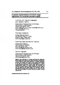
registration is a set of LDR exposures in the Yxy color space. Such a set consists of exactly one base frame at full resolution and a number of smaller re-exposures captured at different points in time. The task of image registration is now to estimate the camera motion that occurred between the exposures so that pixel correspondences can be established. We argue that a purely translational camera motion model is sufficiently accurate for high frame rates. This assumption is supported by [5]. In our approach, the output of image registration is a set of two-dimensional integer vectors describing the shift between the base frame and each re-exposure. The fully registered exposure set is then merged into a single HDR frame. This step includes an implementation of ghost removal to compensate for scene motion that is not covered by image registration. The last step in the chain is tone mapping of the HDR frame. The dynamic range of the frame is compressed to be displayable on a LDR display. 3. HISTOGRAM-BASED IMAGE REGISTRATION This Section describes our histogram-based algorithm for image registration. It solely operates on the brightness channel of the images. The input to our algorithm is a set of n exposures consisting of one full resolution base frame I0 and smaller re-exposures Ii for i = 1, ..., n − 1 captured at different exposure settings. Each re-exposure was initiated by badly exposed regions detected during the analysis of an already captured frame. The analyzed frame can thus be considered the parent frame of the re-exposure. The base frame is the root of the whole set. Each exposure is contained entirely in its parent. Our algorithm performs no image registration on the base frame of an exposure set. Each re-exposure is registered with respect to its parent, i.e., a two-dimensional integer translation vector ~vi between frames Ii−1 and Ii is estimated. Without loss of generality, we assume that exposure Ii−1 is the parent of Ii . By summing up all vectors along the path from an exposure Ii to the base frame, an absolute shift between each exposure and the base frame can be easily calculated. For estimating the translation vectors, we use mean threshold bitmaps (MTB) as described in [5]. A mean threshold bitmap is a black and white image that was created from a greyscale image such that 50% of the image pixels are white and 50% are black. The advantage of an MTB compared to a regular grayscale image is that – within certain limits – two exposures depicting the same scene captured at two different exposure settings will result in approximately the same MTB. This fact is very desirable for image registration. The creation of MTBs is covered in Section 3.1. Once the MTBs of two exposures to be registered are computed, we proceed by computing a column histogram, counting the number of black pixels in each column of the MTB. This is demonstrated in Figure 1. Such a column his-
Fig. 1. Mean Threshold Bitmap of an LDR frame and its corresponding column histogram counting black pixels. togram is computed for both MTBs. By using normalized cross correlation between the two column histograms, we estimate the horizontal component of the translation vector. Repeating this process for image rows allows us to estimate the vertical component respectively. More details on the computation are given in Section 3.2. As a last step, all resulting vectors are validated using a Kalman filter to incorporate knowledge of the prior motion into the estimation. A novel certainty criterion is used to determine the weighting between using the computed translation directly and extrapolating it from the preceding trajectory. This process is described in Secion 3.3. 3.1. Mean Threshold Bitmap Image registration starts with the creation of two MTBs for the two exposures Ii−1 and Ii to be registered. Since a reexposure is always contained entirely in its parent, processing time can be reduced by computing the full MTB of the reexposure Ii , but only computing the MTB of the overlapping image area in the parent frame Ii−1 . The first step is to build a regular histogram with 256 bins over the brightness values of Ii . From the histogram, we can deduce the median brightness value mi to be used as a threshold so that 50% of the thresholded pixels are white and 50% black. At this point, the exposure values (e.g., shutter values) ei−1 , ei at which the two frames were captured as well as the response function f of the capturing camera are known. The response function maps the amount of light incident upon a cell of the CCD sensor onto a pixel value. We can thus use these known values to calculate the unknown threshold mi−1 as follows: mi−1 = f (f −1 (mi )/ei ∗ ei−1 ).
(1)
This is an improvement over the original algorithm and saves the computation of a histogram over Ii−1 .
In the original paper, ignoring pixels with a value near the median is suggested because they are unstable with regard to thresholding. In our experiments, we found that a noise threshold of T = 2 brightness steps below and above the mean leads to good results. For our algorithm, it is sufficient to calculate the two medians mi−1 and mi which are then used to build the row and column histograms. The MTB itself is not built.
The s producing the highest correlation value is then used as the estimate for xi . Using row histograms, the vertical shift yi can be estimated analogously. Our experiments show that the choice of which dimension to start with has little effect on the final result. We also found that performing multiple iterations of the greedy algorithm does not improve the registration quality significantly. We therefore only estimate xi and yi once and set ~vi = (xi , yi ) as the resulting translation vector.
3.2. Row and Column Histograms We estimate a two-dimensional shift ~vi = (xi , yi ) between two exposures Ii−1 and Ii by estimating two one-dimensional shifts xi and yi separately. It is a greedy algorithm for image registration where each dimension of the shift vector is estimated independently of the other. We start by estimating the horizontal shift xi . The first step in doing so is to build column histograms over the full image Ii and the overlapping image area of Ii−1 . A bin in the column histogram represents the number of black pixels in the corresponding column of the exposure’s MTB. Since near-median pixels are ignored as described in the previous Section, two individual histograms counting black and white pixels respectively must be built for each exposure. Let wi and hi be the width and height of Ii . The column histogram Bix (j) of exposure Ii counting black pixels is a function of the column index j = 1, ..., wi and is defined as Bix (j) = |{Ii (j, k) < mi − T ; k = 1, ..., hi }|
(2)
where Ii (j, k) is the pixel value at position (j, k) and | · | denotes the number of elements in the set. The histogram Wix counting white pixels and the two histograms for Ii−1 are defined accordingly. The horizontal shift xi is now estimated using these four histograms. We let the shift s assume all possible integer values within a search range (e.g., -64 to 64 pixels) and compute the normalized cross correlation (NCC) between the histograms of exposures Ii−1 and Ii under the given shift: N CC(s) = √
C N1 N2
(3)
wi X
x x Wix (j)Wi−1 (j − s) + Bix (j)Bi−1 (j − s)
�
(4)
j=1
and N1 and N2 are the two normalization values N1 N2
=
=
wi X j=1 wi X j=1
Wix (j)2 + Bix (j)2
A Kalman filter is used to incorporate the entire trajectory of the camera motion into the estimate of the current frame. For this purpose, we developed a criterion that allows us to judge the certainty of the estimate of ~vi . It is simple and yet performs well – as will be seen in Section 4. From manually registered HDR test videos, we computed mean µ and standard deviation σ of the distances d between two consecutive motion vectors: d = |~vi−1 − ~vi |. With approximately zero mean and assuming that the distances are Gaussian distributed, over 99% of the motion vectors lie within 3σ from the previous vector. At the same time, erroneous measurements can be assumed to be uniformly distributed over the entire search range. We thus use d as criterion for the certainty of the measured shift. A d > 3σ is likely to indicate an incorrect measurement, and the corresponding shift vector is discarded. If d ≤ 3σ, the state of the Kalman filter is updated using ~vi as the measured state and d as the variance of the measurement. In both cases, we use the current state of the filter as the shift vector of the frame to be registered. The state is also used to predict the motion vector ~vi+1 . It helps to improve the performance of the greedy search algorithm and allows to calculate d for the next frame. In our scenario, increasing the search range also increases the chance to detect errors in the shift measurement. Since computing the NCC is rather cheap, we set our search range to approximately ±20σ to leave enough room for error detection. 4. EXPERIMENTAL RESULTS
where C is the cross correlation value between the histograms of Ii−1 and Ii C=
3.3. Kalman Filtering
�
� x x Wi−1 (j − s)2 + Bi−1 (j − s)2 .
(5)
(6)
For our experiments, we captured five HDR test videos – both with and without using a tripod. The videos consist of three indoor and two outdoor shots of mainly static scenes with a large amount of camera rotation. All videos have a resolution of 640 × 480 and an average of 87 HDR frames. Each HDR frame was created using one base frame and 3.35 reexposures on the average. The first two videos were used to fine-tune the parameters of the algorithm (e.g., search range, noise threshold T , uncertainty threshold for d). All five videos are used for performance evaluation. All frames were registered manually, and the resulting translation vectors constitute the ground truth for evaluating the accuracy of our automatic
Ward 1.56 (3.46) 1.05 (2.21) 1.37 (4.05) 2.27 (4.70) 3.96 (6.33)
without filtering 5.21 (6.90) 1.31 (1.49) 1.12 (3.47) 1.78 (3.76) 4.52 (6.69)
with filtering 1.12 (2.60) 1.13 (0.89) 0.78 (0.78) 1.38 (1.37) 2.77 (2.89)
Fig. 2. Average registration error (and standard deviation in brackets) for the five test videos. The algorithms compared are: Ward’s algorithm, our approach without filtering and our full algorithm. algorithm. As the criteria for our evaluation, we use mean and standard deviation of the distance between our estimate and the ground truth over all frames of a video. Since it is our goal to capture and display HDR videos in real-time, the time taken for registration of a frame of a certain size is our second criterion. Both criteria are compared to our implementation of Ward’s algorithm [5]. Ward’s algorithm was developed for registering still images only. It does not make use of the history of motion vectors. So we start by comparing its accuracy to the one achieved by the still image version of our algorithm, excluding the filtering and prediction. The search range is set to 16 for both approaches. The second and third column of the table in Figure 2 show the results of this comparison. It can be seen that in this setup both algorithms perform similarly with respect to accuracy. The first video contains re-exposures with a height of only 48 pixels which is too small for our algorithm to handle properly. Video 5 is an indoor scene with motion blur in some of the long exposures. This explains the bad accuracy achieved by both. In the second step, we add Kalman filtering to our approach and set the search range to 64. The rightmost column of the table indicates the accuracy improvement achieved. The effect of filtering outliers can be seen best in the reduced standard deviation. The motion vectors of the small frames of video 1 are now interpolated from the surrounding bigger frames, leading to a much better accuracy. Figure 3 shows the time taken for both algorithms to perform image registration. Since for both algorithms the image content does not influence the speed, we conducted all time measurements on a random frame and registered it with itself. The HDR capturing algorithm we employ always captures re-exposures at full width but with varying height [1], so the frame was cropped to heights from 100 to 480 pixels in steps of 10 before registration. Depending on the frame size, Ward’s algorithm takes between 1.4 and 3 times longer than ours. At full resolution, approximately 7.3 out of the 8 ms taken by our algorithm are due to the computation of means and the construction of row and column histograms. Only 0.7 ms are taken for computing the normalized cross correlation. Filtering the results takes approximately 0.016 ms and is negligible.
12 Processing time [ms]
Video # 1 2 3 4 5
10 8 6 4 2
Ward Image Registration Our Approach
0 100
150
200
250 300 350 Frame height [pixel]
400
450
Fig. 3. Time taken for registration of images with a width of 640 pixels and the given height. 5. CONCLUSION AND OUTLOOK We introduced an approach to the registration of LDR exposures for the creation of HDR videos in real-time. The focus was on improved registration speed compared to existing algorithms. We believe that the accuracy achieved by our algorithm using Kalman filtering is acceptable in most viewing scenarios. The biggest obstacles for further accuracy improvement are the assumptions of purely translational motion and integer-valued motion vectors. The former is an inherent part of our algorithm. However in future work, we would like to add sub-pixel shift measurements to our approach to overcome the 0.5 pixels of average quantization error immanent to our implementation. We would also like to explore the possibility of registering different pairs of exposures than just a frame and its parent. 6. REFERENCES [1] B. Guthier, S. Kopf, and W. Effelsberg, “Capturing high dynamic range images with partial re-exposures,” in IEEE 10th Workshop on Multimedia Signal Processing, 2008, pp. 241–246. [2] S.B. Kang, M. Uyttendaele, S. Winder, and R. Szeliski, “High dynamic range video,” in ACM Transactions on Graphics 22(3), 2003, pp. 319–325. [3] B. Guthier, S. Kopf, and W. Effelsberg, “High-resolution inline video-aoi for printed circuit assemblies,” in Proceedings of IS&T/SPIE Electronic Imaging, 2009. [4] P.M.Q. Aguiar, “Unsupervised simultaneous registration and exposure correction,” in Proc. of IEEE ICIP, 2006, pp. 361–364. [5] G. Ward, “Fast, robust image registration for compositing high dynamic range photographs from handheld exposures,” in Journal of Graphics Tools, 8(2), 2003, pp. 17–30.