Histogram-based method for contrast measurement Luis Miguel Sanchez-Brea, Juan Antonio Quiroga, Angel Garcia-Botella, and Eusebio Bernabeu
A histogram-based technique for robust contrast measurement is proposed. The method is based on fitting the histogram of the measured image to the histogram of a model function, and it can be used for contrast determination in fringe patterns. Simulated and experimental results are presented. © 2000 Optical Society of America OCIS codes: 100.0100, 100.2650, 100.2960.
1. Introduction
Contrast measurement is a useful tool for the measurement of the modulation transfer function 共MTF兲 of an optical system. A direct method for determining the MTF is by measuring the contrast of several sinusoidal fringe patterns with different spatial frequencies imaged by the optical system under test. However, since sinusoidal patterns are difficult to obtain, usually the MTF is indirectly measured with Ronchi patterns. This gives an estimation of the contrast transfer function 共CTF兲. By means of a modal expansion of the square pattern, it is possible to obtain a relationship between the CTF and the MTF, and when this relationship is inverted, the MTF can be measured in terms of the CTF,1,2
MTF共 f 兲 ⫽
冋
CTF共3f 兲 CTF共5f 兲 CTF共 f 兲 ⫹ ⫺ 4 3 5 ⫹
册
CTF共7f 兲 ⫹··· , 7
(1)
´ ptica, Universidad The authors are with the Departamento de O Complutense de Madrid, Facultad de Ciencias Fı´sicas, Cuidad Universitaria s兾n, 28040 Madrid, Spain. When this research was performed, J. A. Quiroga was with the Centro de Investigaciones ´ ptica, Apartado Postal 1-948, 37000 Le´on GTO, Me´xico. en O L. M. Sanchez-Brea’s e-mail address is
[email protected]. ucm.es. Received 13 October 1999; revised manuscript received 27 March 2000. 0003-6935兾00兾234098-09$15.00兾0 © 2000 Optical Society of America 4098
APPLIED OPTICS 兾 Vol. 39, No. 23 兾 10 August 2000
where f is the frequency. In the absence of noise and for a periodic signal the straightforward definition of contrast is C⫽
IMAX ⫺ IMIN , IMAX ⫹ IMIN
(2)
where IMAX and IMIN are the maximum and the minimum values of the signal. When noise or small background variations are present, it is not possible to apply this definition directly. If the image from which we wish to determine the contrast is formed by a straight-line pattern, one possibility is to align the pattern 共by digital or optical methods兲 parallel to one of the reference axes and then sum along it. In this way the averaging will reduce the noise, enabling the measurement of IMAX and IMIN. Unfortunately this simple method has big drawbacks, especially if mediumlow contrasts are to be measured 共C ⬇ 0.5–0.1兲. In addition, the determination of IMAX and IMIN by a simple averaging is sensitive to noise and兾or to small background variations. Furthermore, this method cannot be applied when fringes become curved after passing through the optical system or for circular fringes, which can be used for the determination of directional MTF when we analyze a small slit of the image at the proper direction. Another way to evaluate the contrast of a fringe pattern is by use of the histogram, as suggested by Lai and von Bally.3 However, the algorithm they propose does not match the definition of contrast 关Eq. 共2兲兴 even when no noise is present. In this study we propose a histogram-based technique for contrast measurement of fringe patterns that can be applied in the presence of additive noise and with patterns composed of fringes that are not straight. The method is based on fitting the histogram of the measured fringe pattern to the histogram of a model func-
tion that depends on several parameters. The parameters of the model function provide information about contrast and noise level. By means of histogram analysis we can obtain more information about fringes, besides contrast. Generally histograms of fringe patterns present two lobes, but square and sinusoidal fringe patterns with the same contrast do not have the same histogram shape. From this difference, information about the fringe shape can be obtained. This paper is organized as follows: In Section 2 we show how to calculate the histogram of the chosen model function and how to extract the contrast information from an experimental fringe pattern by use of this model function. In Section 3 we apply the algorithm to simulated fringe patterns. In Section 4 experimental results with real fringe patterns are obtained. Finally in Section 5 conclusions are given. 2. Contrast Measurement from the Histogram
The continuous histogram h共 y兲 of a continuous function f 共x兲 can be defined as the number of points that fulfill y ⱕ f 共兲 ⬍ y ⫹ dy. The mathematical expression of this definition is h共 y兲 ⫽
兰
␦关 f 共x兲 ⫺ y兴dx,
(3)
⍀
where ␦ stands for the Dirac-delta function and ⍀ is the set of points x where we are computing the histogram. The Dirac-delta function of a continuous function g共x兲 is4 ␦关 g共x兲兴 ⫽
1
兺 兩 g⬘兩 ␦共x ⫺ x 兲, i
(4)
i
where g⬘ represents derivative of g with respect to x, 兩 䡠 兩 means absolute value, xi are the roots of g共x兲, and i is an index that runs over them. Then, if we consider g共x兲 ⫽ f 共x兲 ⫺ y,
(5)
by applying Eqs. 共3兲 and 共4兲 and taking into account that the root of Eq. 共5兲 is x ⫽ f ⫺1共 y兲, we obtain
兰
1 ␦关 x ⫺ f ⫺1共 y兲兴dx, h共 y兲 ⫽ 兩 f⬘兩 ⍀
(6)
or h共 y兲 ⫽
1 ⫺1
兩 f⬘关 f 共 y兲兴兩
.
冏
冏
df ⫺1共 y兲 . dy
h共 y兲 ⫽
再
1兾兩关b2 ⫺ 共 y ⫺ a兲2兴1兾2兩 0
a⫺b⬍y⬍b⫹a . elsewhere (9)
In this way, when our fringe pattern corresponds to lines of any shape with sinusoidal profile, we can fit its histogram with the one given by Eq. 共9兲, and from the fitting parameters we can obtain the contrast by C ⫽ 兩b兾a兩. However, if we use Ronchi rulings to determine the CTF of an optical system, this simple scheme does not work properly because of noise in the fringe pattern and discontinuities of the model, as explained in Subsections 2.A–2.D. A.
Histogram of a Noisy Signal
When a fringe pattern is obtained by means of a CCD camera or by other procedures, there always exists noise that modifies the histogram shape. We will assume an additive noise n共r兲 whose probability distribution is p共 y兲, where r is the position vector. The histogram h共 y兲 of the fringe pattern I共r兲 can be considered to be the probability distribution of the intensity values. Thus the histogram of a noisy image, I 共r兲 ⫽ I共r兲 ⫹ n共r兲,
(10)
will be the probability distribution of a signal composed by the sum of two signals with probability distributions h共 y兲 and p共 y兲. From probability theory5,6 it can be proved that the histogram of I 共r兲 is h 共 y兲 ⫽ h共 y兲 ⴱ p共 y兲,
(11)
where ⴱ denotes the convolution product. Then, by selecting a model for the additive noise, we can determine the histogram of the selected model with additive noise as the convolution product of the model histogram with the noise histogram.
(7) B.
Expression 共7兲 can be rewritten, by means of the inverse function theorem, as h共 y兲 ⫽
ues of y.5 From Eq. 共6兲 it is clear that the conditions for f 共x兲 to have a histogram are the existence of the inverse function f ⫺1共 y兲 and the absence of extrema of f 共x兲 within ⍀. For these reasons, in the case of periodic functions, we cannot directly apply Eqs. 共7兲 or 共8兲. To compute the histograms, we must use only one semiperiod between a minimum and a maximum and multiply the histogram by the number of semiperiods present. For instance, to compute the continuous histogram of f 共 x兲 ⫽ a ⫹ b cos共wx兲, a ⬎ b, we use the interval ⍀ ⫽ 共0, 兾w兲 where no extrema are present and f ⫺1共 y兲 is defined. Then, applying Eq. 共7兲, we obtain
(8)
Equations 共7兲 and 共8兲 are a well-known result of the theory of probability if we interpret the histogram of a function as the probability distribution for the val-
Elimination of Divergences
Another problem of the continuous histogram 关Eq. 共7兲兴 are the divergences that exist near the extrema of the model, where f⬘共 x兲 ⫽ 0. The presence of these divergences destabilizes the minimization algorithm necessary for the fitting process, making it difficult and unreliable. We solved this problem by using a sampled model instead of a continuous one. For a sampled model with M samples it is clear that the histogram will never diverge, the fitting making eas10 August 2000 兾 Vol. 39, No. 23 兾 APPLIED OPTICS
4099
ier and more reliable. This solution is not really an approximation, since any digital image acquisition system imposes a spatial sampling and an intensity quantization. The first step to compute the discrete histogram of a sampled function is to define the range of values for the intensities and the domain of the sampled function. The possible values for the intensities are yn ⫽ 共n ⫺ 1兲⌬y,
n ⫽ 1, . . . , N,
(12)
where ⌬y is the difference between two adjacent intensity levels and we are assuming that the lowest value for the intensity is 0. The domain ⍀, where the sampled function is defined, is given by a uniform sampling, xm ⫽ x1 ⫹ 共m ⫺ 1兲⌬x,
m ⫽ 1, . . . , M,
(13)
where x1, ⌬x, and M are free parameters that determine this sampling. The discrete histogram h关n兴 共where the square brackets indicate that the discrete histogram can have only positive integer values兲 of the sampled
The ⫹1 added to h关nMAX兴 is to take into account the final point 关 xM, f 共 xM兲兴. From Eq. 共15兲 it is easy to verify that N
兺 h关n兴 ⫽ M,
where M is the total number of sampling points. Then Eqs. 共15兲 and 共16兲 define the way a discrete histogram of a sampled function can be computed. However, working with integer parts and absolute values is not comfortable from the viewpoint of the analysis, so we are going to define a continuous histogram of a sampled model function, h共n兲, from its discrete counterpart, h关n兴. To eliminate the absolute values, we are going to consider only model functions f 共x兲 monotonically increasing in the range 关 x1, xM兴. This is not a lack of generalization, because the histogram of a monotonically decreasing function is the same as the corresponding mirror reflection about the vertical axis. With this consideration and when the integer parts of Eq. 共15兲 are eliminated, the continuous histogram of the sampled function, h共n兲, is
冦
关 f ⫺1共 ynMIN ⫹ ⌬y兾2兲 ⫺ x1兴兾⌬x 关 f ⫺1共 yn ⫹ ⌬y兾2兲 ⫺ f ⫺1共 yn ⫺ ⌬y兾2兲兴兾⌬x h共n兲 ⫽ 关 xM ⫺ f ⫺1共 ynMAX ⫺ ⌬y兾2兲兴兾⌬x ⫹ 1 0 function f 共 xm兲 is defined as the number of points xm such that y1 ⱕ f 共xm兲 ⬍ y1 ⫹ ⌬y兾2,
n ⫽ nMIN nMIN ⬍ n ⬍ nMAX , n ⫽ nMAX elsewhere
N
1 ⬍ n ⬍ N,
yN ⫺ ⌬y兾2 ⱕ f 共xm兲 ⬍ yN,
n ⫽ N.
(14)
With this definition h关n兴 is basically calculated by means of counting the number of points xm in the interval 关 f ⫺1共 yn ⫺ ⌬y兾2兲, f ⫺1共 yn ⫹ ⌬y兾2兲兴, that is,
兺 h共n兲 ⫽ M,
so no divergences appear as long as f ⫺1共 yn兲 exists. Also, in the limit ⌬x 3 0, ⌬y 3 0, Eq. 共18兲 is the link between the discrete histogram of a sampled function and the corresponding continuous histogram of a con-
冦
where int共x兲 denotes the integer part of x and nMAX and nMIN are the first and the final indices with h关n兴 different from 0. They are computed by nMAX ⫽ int关 f 共xM兲兾⌬y兴 ⫹ 1,
APPLIED OPTICS 兾 Vol. 39, No. 23 兾 10 August 2000
n ⫽ nMIN nMIN ⬍ n ⬍ nMAX , n ⫽ nMAX elsewhere
(15)
tinuous function given by Eqs. 共7兲 and 共8兲. Thus Eq. 共18兲 is the expression of the histogram we adopted to make the calculations. Figure 1 shows the relation between h关n兴 and h共n兲 for the model function f 共x兲 ⫽ a ⫹ b cos共wx兲 with b ⫽ 75, a ⫽ 125; x1 ⫽ 0, xM ⫽ 兾w, and M ⫽ 300. C.
(16)
(19)
n⫽1
兩int关 f ⫺1共 ynMIN ⫹ ⌬y兾2兲兾⌬x兴 ⫺ int共x1兾⌬x兲兩 兩int关 f ⫺1共 yn ⫹ ⌬y兾2兲兾⌬x兴 ⫺ int关 f ⫺1共 yn ⫺ ⌬y兾2兲兾⌬x兴兩 h关n兴 ⫽ 兩int共xM兾⌬x兲 ⫺ int关 f ⫺1共 ynMAX ⫺ ⌬y兾2兲兾⌬x兴兩 ⫹ 1 0
4100
(18)
where nMAX and nMIN are defined by Eq. 共16兲. Again, from Eq. 共18兲 it is easy to verify that
n ⫽ 1,
yn ⫺ ⌬y兾2 ⱕ f 共xm兲 ⬍ yn ⫹ ⌬y兾2,
nMIN ⫽ intf 关共x1兲兾⌬y兴 ⫹ 1.
(17)
n⫽1
Model Function
Once we know how to account for the effect of the noise in the histogram of the model function 关Eq.
共11兲兴, and how to manage the divergences appearing in the continuous definition of the histogram 关Eq. 共18兲兴, the next step is to select a suitable model function able to adapt to a variety of profiles, from highcontrast square patterns to almost pure sinusoidal patterns, considering a continuous grading of shapes from square to sinusoidal. The simple sinusoidal model function of Eq. 共9兲 is not flexible enough to accomplish all this phenomenology. A good candidate for this, and the one we finally adopted, was the sigmoidal function fS共x兲 given by fS共x兲 ⫽ a ⫹
b⫺a , 1 ⫹ exp关⫺共x ⫺ x0兲兾兴
(20)
where a and b are parameters that control the maximum and the minimum values of fS共x兲, x0 is a parameter that controls the possible lateral shift, and is the parameter that controls the shape: As grows, fS共x兲 changes from a step function to a sinusoidallike function. Then, as explained above for periodic signals, fS共x兲 will represent an approximation of one semiperiod. The continuous histogram of fS共x兲 is, when we apply Eq. 共7兲 or Eq. 共8兲,
再
共b ⫺ a兲兾关共b ⫺ y兲共 y ⫺ a兲兴 y 僆 共a, b兲 hS共 y兲 ⫽ . (21) 0 elsewhere As can be seen in Eq. 共21兲, divergences appear in y ⫽ a and y ⫽ b, making it difficult to be used as a fitting function 共as explained above兲. When we take into account that the inverse function of fS共x兲 is
冉 冊
fS⫺1共 y兲 ⫽ x0 ⫺ ln
y⫺b , a⫺y
where we have explicitly written the free parameters of the model and p共n, 兲 is the sampled version of Eq. 共24兲 obtained by changing of the continuous variable y with yn given by Eq. 共12兲. D.
Calculation of Contrast Parameters
The final step in the proposed method for contrast measurement is the calculation of the parameters a, b, , x0, and that minimize the functional E given by N
(22)
E⫽
兺 兵h 关n兴 ⫺ h 共n, a, b, , x , 兲其 , 2
D
冎再
where nMIN and nMAX are given by Eq. 共16兲. We have assumed the additive noise to be Gaussian, with zero mean, since it is easily tractable. Then its probability distribution will be
冉 冊
y2 p共 y, 兲 ⫽ exp ⫺ 2 , 2 冑2 1
(24)
and then the model histogram for the sigmoidal function with additive Gaussian noise incorporated in the model will be, when we apply Eq. 共11兲, h S共n, a, b, , x0, 兲 ⫽ hS共n兲 ⴱ p共n, 兲,
0
(26)
where hD关n兴 is the discrete histogram of the experimental data to be analyzed, with its maximum nor-
关 fS⫺1共 ynMIN ⫹ ⌬y兾2兲 ⫺ x1兴兾⌬x ⌬y ⌬y ln 1 ⫹ 1⫹ hS共n兲 ⫽ ⌬x 关b ⫺ 共n ⫺ 1兾2兲⌬y兴 关共n ⫺ 3兾2兲⌬y ⫺ a兴 兵 xM ⫺ fS⫺1共 ynMAX ⫺ ⌬y兾2兲其兾⌬x ⫹ 1 0
(再
S
n⫽1
the continuous histogram of the sampled version of fS共x兲 is
冦
Fig. 1. Relationship between h关n兴 共circles兲 and h共n兲 共diamonds兲 for f 共x兲 ⫽ a ⫹ b cos共wx兲, with b ⫽ 75, a ⫽ 125, x1 ⫽ 0, xM ⫽ 兾w, and M ⫽ 300. Only one of each of the four points is presented to improve the visibility of the figure.
(25)
冎)
n ⫽ nMIN nMIN ⬍ n ⬍ nMAX
,
(23)
n ⫽ nMAX elsewhere
malized to 1. From the parameters obtained in the minimization of Eq. 共26兲 the contrast of the image with the histogram is C⫽
fS共xM兲 ⫺ fS共x1兲 . fS共xM兲 ⫹ fS共x1兲
(27)
When the noise is independent of the intensity values, Eq. 共26兲 resumes our contrast measurement method. However, in real experiments we observed an intensity dependence on the noise level. We expect that the development of a model with multiplicative noise will solve this problem. Nonetheless, 10 August 2000 兾 Vol. 39, No. 23 兾 APPLIED OPTICS
4101
Fig. 2. Simulated one-dimensional fringe patterns with additive noise and different fringe profile: 共a兲 for a sine fringe pattern, 共b兲 quasi-sine fringe pattern, 共c兲 quasi-square fringe pattern. For all cases a ⫽ 50, b ⫽ 200, ⫽ 15 g.l. 共d兲, 共e兲, 共f 兲: circles, histograms obtained from 共a兲, 共b兲, 共c兲, respectively; curve, fits to sigmoidal histogram by means of minimization of Eq. 共26兲.
we adopted a strategy based on the additive noise model, which consists of dividing the histogram of a noisy model function into two parts and using two noise levels 1 and 2 for each one. We implemented this idea by means of a weighting function ⌳共n兲, defined as a step function with a linear transition zone of width ⌬n ⫽ int关␣共b ⫺ a兲兴 gray levels and centered at n ⫽ int关共a ⫹ b兲兾2兴. The parameter that controls the width of the transition zone is typically ␣ ⫽ 0.1. Finally, the histogram for the sigmoidal function with two levels of additive noise will be h S共n, a, b, , x0, 1, 2兲 ⫽ ⌳共n兲关hs共n兲 ⴱ p共n, 1兲兴 ⫹ 关1 ⫺ ⌳共n兲兴关hs共n兲 ⴱ p共n, 2兲兴, (28) 4102
APPLIED OPTICS 兾 Vol. 39, No. 23 兾 10 August 2000
and the parameters are determined by the minimization of N
E⫽
兺 兵h 关n兴 ⫺ h 共n, a, b, , x , , 兲其 . 2
D
S
0
1
2
(29)
n⫽1
From Eq. 共23兲 it can be seen that Eqs. 共26兲 and 共29兲 are nonlinear minimization problems. Many algorithms exist to perform this task. In particular we used the Nelder–Mead-type simplex algorithm implemented in the optimization toolbox of the Matlab environment.7 In general the successful minimization of a nonlinear problem needs good starting values for the parameters involved. In our case the best results were obtained with the following rules for selecting the starting values. When hD关n兴 is bimodal,
Table 1. Estimated Parameters for Fringe Profiles of Fig. 2 with a Histogram-Based Method
Parameter Figure
a*
b*
fS共x1兲*
fS共xM兲*
C
x0*
*
2共a兲 2共b兲 2共c兲
50.67 53.07 52.35
203.59 204.41 198.50
54.01 53.36 52.35
200.25 204.12 198.50
0.575 0.586 0.583
0.06 ⫺0.07 0.03
0.263 0.160 0.0308
14.77 12.42 15.67
*Gray levels.
a and b are initialized as the gray values that correspond to each maximum of hD关n兴. If hD关n兴 presents only one lobe, whose maximum is located in the gray value G, the parameters a and b are initialized as G ⫺ ⌬G and G ⫹ ⌬G, with ⌬G typically 4.
The shape parameter is initialized as hD关共na ⫹ nb兲兾2兴, where na and nb are the indices of the gray values a and b previously initialized. If the histogram hD关n兴 is too noisy, local averaging centered on n ⫽ 共na ⫹ nb兲兾2 is done for the calculation of hD关共na ⫹ nb兲兾2兴. Finally, the parameter x0 is initialized to 0, and the parameters 1 and 2 are initialized as the width at half the height of each of the lobes if the histogram is bimodal. If the histogram is monomodal 1 and 2 are initialized as the corresponding width of the unique lobe. 3. Application to Simulated Patterns
The algorithm depicted above was applied to three simulated fringe patterns with added noise, as shown in Fig. 2. Since we are working with 256 gray levels 共g.l.兲 in all these cases, then N ⫽ 256, ⌬y ⫽ 1, and thus yMIN ⫽ 0 and yMAX ⫽ 255. We arbitrarily fixed x1 ⫽ ⫺1, xM ⫽ 1, ⌬x ⫽ 10⫺3, M ⫽ 2001, for all our measurements. Figures 2共a兲–2共c兲 show the fringe patterns that range from a sinusoidal to a square profile shape. In the three cases the actual contrast is 0.6 共a ⫽ 50, b ⫽ 200兲, x0 is zero, and the noise standard deviation is 15 g.l. The corresponding histograms and the result of the minimization of Eq. 共26兲 are shown in Figs.
Fig. 3. Simulated 共thin兲 and estimated 共thick兲 fringe shape for the fringe patterns given in Fig. 1. The estimated fringe shape is obtained from results of Table 1. As we can see, there is a good agreement between the simulated and the estimated profiles.
Fig. 4. Estimated uncertainty for contrast estimation in terms of Gaussian noise for several fringe shapes: 共inverted triangles兲 ⫽ 0.263; 共asterisks兲 ⫽ 0.160; 共circles兲, ⫽ 0.0308. In this case the contrast is C ⫽ 0.6 共a ⫽ 50, b ⫽ 200兲. 10 August 2000 兾 Vol. 39, No. 23 兾 APPLIED OPTICS
4103
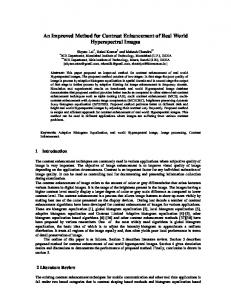
Fig. 6. Sketch of the experimental setup for contrast measurement of bar tests when a translucent rough sheet is interposed between the bar test and the CCD camera.
separated lobes in the histogram. As a consequence it is easier for the minimization algorithm to detect them correctly. In the case of the sinusoidal and the quasi-sinusoidal patterns the lobes are not so well resolved, making it more difficult to determination their positions correctly as the noise increases. We also carried out an experiment that consists of modifying the number of fringes per frame to show that the fitting parameters do not depend on the spatial frequency of the output signal, especially the parameter that accounts for the fringe shape. We obtained that the spatial frequency of the signal affects only the histogram as a scaling factor. In Fig. 5共a兲 we show the parameter in terms of the number of fringes per frame for three different fringe profiles. As we can see, is constant for the three cases, except for a small fluctuation that is due to noise. A contrast estimation in terms of the number of fringes was also carried out 关Fig. 5共b兲兴. For the three simulations the contrast is approximately the same. Fig. 5. 共a兲 Estimation of in terms of the number of fringes per frame for three different shape profiles, 共b兲 estimation of contrast for the same cases. The theoretical contrast is C ⫽ 0.6, and a noise of 10 g.l. has been added.
2共d兲–2共f 兲. Visually the fit is good; and also numerically, as shown in Table 1. Figure 3 represents half a period of the simulated profiles of Fig. 2 together with the sigmoidal function 共20兲 evaluated for the corresponding parameters shown in Table 1. The profiles depicted in Figs. 3共a兲, 3共b兲, and 3共c兲 correspond to the simulated profiles of Figs. 2共a兲, 2共b兲, and 2共c兲, respectively. In this example we can see that the sigmoidal model function adapts well from sine to square fringes. To determine the performance of the algorithm we estimated the contrast in terms of the noise level for three different shapes: sinusoidal, quasi sinusoidal, and almost square. For each level of noise and profile shape we estimated the contrast ten times and calculated the mean relative error. In Fig. 4 the mean relative error is represented in terms of the relative error. As can be seen, the error for the square-shaped profile is less that the one corresponding to the sinusoidal and the quasi-sinusoidal ones. The reason for that behavior is that the square profile has well-defined populations that produce two well4104
APPLIED OPTICS 兾 Vol. 39, No. 23 兾 10 August 2000
4. Experimental Results
In this section we show the results of the application of the algorithm depicted above to determine the CTF of an optical system. Our particular interest was the measurement of the MTF of translucent rough screens. The first step of the method we are using is the measurement of the CTF and afterward estimation of the MTF1 from the CTF measurement. The optical setup for the measurement of the CTF is shown in Fig. 6. The light produced by a halogen lamp is directed to the input port of an integrating sphere such that at the output port we have a nearly uniform white-light beam that is localized on a diaphragm by means of an achromatic doublet. The light emerging from the diaphragm is collimated by means of another achromatic doublet and directed to a Ronchi bar test that is projected on a rough translucent screen. The transmitted pattern is imaged on a bidimensional CCD camera by means of a third achromatic doublet. The CCD performs an 8-bit quantization 共256 g.l.兲, and then N ⫽ 256, ⌬y ⫽ 1, yMIN ⫽ 0, yMAX ⫽ 255. For the sampling of the sigmoidal function we used x1 ⫽ ⫺1, xM ⫽ 1, ⌬x ⫽ 10⫺3, M ⫽ 2001. As an example, in Fig. 7 we can see the application of the algorithm to three real images. Figures 7共a兲– 7共c兲 are profiles from the images recorded by the CCD
Fig. 7. Profiles from two-dimensional real fringe patterns and fits for their histograms: 共a兲 and 共d兲 sinusoidal low-contrast pattern, 共b兲 and 共e兲 sinusoidal high-contrast pattern, and 共c兲 and 共f 兲 square high-contrast pattern. Only one of each of the four points is presented to improve the visibility of 共d兲–共f 兲. Circles, experimental histogram; curve, the fit.
camera, and figures 7共d兲–7共f 兲 are the experimental histograms of the corresponding images together with the results of the minimization of Eq. 共29兲. Especially remarkable is the example of Figs. 7共a兲 and 7共d兲; in this case the maxima of the contrast pattern are modulated, producing a lobe whose width is not due to the noise but to the intensity modulation of the maxima. Even in this case the algorithm works well and correctly locates the lobes. This shows that the parameters associated with the noise, 1 and 2, can be interpreted as high-frequency additive noise or as a low-frequency modulation present in the image, or, in general, as a mix of both effects. Table 2 shows the parameters obtained by the fits. Finally we measured the CTF of a translucent rough sheet. The contrast of the observed pattern depends on the period of the bar test h, the separation
between the bar test and the translucent rough sheet d, and its roughness 兾, as shown by Garcia-Botella et al.,8 according to CTF共h, d, 兾兲 ⫽
冉 冊
4 ⬁ 1 共⫺1兲k k⫽0 2k ⫹ 1
兺
再冋
⫻ exp ⫺ 共2k ⫹ 1兲
2 d共n ⫺ 1兲 h
册冎 2
.
(30) In Fig. 8 we can see the fit of our experimental measurements of the CTF 共obtained by the histogram-based method兲 to Eq. 共30兲 in terms of spatial frequency for two values of the separation between the bar test and the sheet: d1 ⫽ 5 cm 共circles兲 10 August 2000 兾 Vol. 39, No. 23 兾 APPLIED OPTICS
4105
Table 2. Estimated Parameters for Measurements of Real Fringe Patterns by Means of a Histogram-Based Method
Parameter Figure 共a兲 共b兲 共c兲
a*
b*
fS共x1兲* fS共xM兲*
C
1*
2*
47.25 77.25 50.65 73.85 0.186 0.486 2.11 1.26 5.64 122.47 6.61 121.50 0.897 0.209 2.25 24.59 0.10 177.35 0.10 177.35 0.999 0.0026 0.55 8.35
*Gray levels.
Fig. 8. Measurements of contrast transfer function by means of histogram-based method, for a dielectric rough sheet with n ⫽ 1.523 and roughness parameter of 兾 ⫽ 165 ⫾ 4, at distances between bar test and sheet of d1 ⫽ 5 cm 共squares兲 and d2 ⫽ 10 cm 共circles兲, compared with the model proposed by Garcia-Botella et al.8
and d2 ⫽ 10 cm 共squares兲. The roughness parameter for the sample was 兾 ⫽ 165 ⫾ 5, measured by profilometry and reflectogoniometry. As can be seen, the agreement between the model and the experimental measurements is good. Especially remarkable is the behavior of the experimental measurements in the tails, where a small peak can be observed 共Fig. 8, circles, at 2 cycles兾mm兲. This behavior is reproducible, so we think that it corresponds to diffraction effects that the geometric model 关Eq. 共30兲兴 does not consider. 5. Conclusions
In this study we have presented a histogram-based technique for robust contrast measurement. The
4106
APPLIED OPTICS 兾 Vol. 39, No. 23 兾 10 August 2000
method is based on the fitting of the histogram of the measured image with the histogram of a model function. Analytical expressions for the histogram of continuous as well as sampled functions were obtained. The selected model function was the sigmoidal function, which was shown to be flexible enough to accommodate a great variety of cases. With this technique contrast measurement can be performed by means of patterns of almost any shape. Finally, experimental measurements of the CTF of an optical system were made in good agreement with the theoretical model. Juan Antonio Quiroga acknowledges the support of a postdoctoral grant of the Universidad Complutense de Madrid and the Becas Internacionales Flores-Valles program, Spain, and Centro de Inves´ ptica, Leo´n, Me´xico. Luis Miguel tigaciones en O Sanchez-Brea acknowledges the support of a predoctoral grant of the Ministerio de Educacio´n y Cultura 共Intercambio de Personal Investigador entre Industrias y Centros Pu´blicos de Investigacio´n兲 with Kinossel S.L. This study was supported in part by Sainco Tra´fico, S.A., in the framework of Proyecto de Estı´mulo a la Transferencia de Resultados de Investigacio´n 共PETRI兲 program, Baliza Luminosa para el Guiado de Tra´fico Vial con Tecnologı´a LED project of the Ministerio de Educacio´n y Cultura. References 1. J. W. Coltman, “The specification of imaging properties by response to a sine wave input,” J. Opt. Soc. Am. 44, 468 – 471 共1954兲. 2. G. C. Holst, CCD Arrays, Cameras, and Displays 共Society for Photo-Optical Instrumentation Engineers, Bellingham, Wash., 1996兲. 3. S. Lai and G. von Bally, “Fringe contrast evaluation by means of histograms,” in OPTIKA ’98: 5th Congress on Modern ´ kos, G. Lupkovics, and P. Andra´s, eds., Proc. SPIE Optics, G. A 3573, 384 –387 共1998兲. 4. J. D. Gaskill, Linear Systems, Fourier Transforms, and Optics 共Wiley, New York, 1978兲. 5. A. Papoulis, Probability, Random Variables, and Stochastic Processes 共McGraw-Hill, New York, 1965兲. 6. B. R. Frieden, Probability, Statistical Optics, and Data Testing 共Springer-Verlag, Berlin, 1983兲. 7. T. Coleman, M. A. Branch, and A. Grace, Optimization Toolbox for Use with MATLAB, users guide version 2 共MathWorks, Natick, Mass., 1996兲. 8. A. Garcia-Botella, L. M. Sanchez-Brea, D. Vazquez-Molini, and E. Bernabeu, “Modulation transfer function for translucent rough sheet,” Appl. Opt. 38, 5429 –5432 共1999兲.