rod, reinforced by their sci-fi side...â (Lotte 2016). ...... Leonardo Duque MuËnoz, Karen J Mullinger, Tim M Tierney, Sven Bestmann, Gareth R. Barnes, Richard ...
HISTOGRAM OF GRADIENT ORIENTATIONS OF EEG SIGNAL PLOTS FOR BRAIN COMPUTER INTERFACES por Rodrigo Ramele
EN CUMPLIMIENTO PARCIAL DE LOS REQUISITOS PARA OPTAR AL GRADO DE DOCTOR EN INGENIER´IA INFORMATICA DEL ´ INSTITUTO TECNOLOGICO DE BUENOS AIRES BUENOS AIRES, ARGENTINA 29 DE NOVIEMBRE, 2018
c Copyright Rodrigo Ramele, 2018
´ INSTITUTO TECNOLOGICO DE BUENOS AIRES
DEPARTAMENTO DE DOCTORADO Los aqu´ı suscriptos certifican que han asistido a la presentaci´on oral de la Tesis “Histogram of Gradient Orientations of EEG Signal Plots for Brain Computer Interfaces” cuyo autor es Rodrigo Ramele completando parcialmente, los requerimientos exigidos para la obtenci´ on del T´ıtulo de Doctor en Ingenier´ıa Informatica.
Fecha: 29 de Noviembre, 2018
Directores: Dr. Juan Miguel Santos
Dra. Ana Julia Villar
Tribunal de Tesis: Dra. Mar´ıa Alejandra Figliola
Dr. Osvaldo Rosso
Dr. Alejandro C. Frery
ii
´ INSTITUTO TECNOLOGICO DE BUENOS AIRES Fecha: 29 de Noviembre, 2018 Autor:
Rodrigo Ramele
T´ıtulo:
Histogram of Gradient Orientations of EEG Signal Plots for Brain Computer Interfaces
Departamento:
Doctorado
T´ıtulo Acad´emico: Doctor en Ingenier´ıa Informatica
Convocatoria: Mes
A˜ no
Por la presente se otorga permiso al Instituto Tecnol´ogico de Buenos Aires (ITBA) para: (i) realizar copias de la presente Tesis y para almacenarla y/o conservarla en el formato, soporte o medio que la Universidad considere conveniente a su discreci´on y con prop´ ositos no-comerciales; y, (ii) a brindar acceso p´ ublico a la Tesis para fines acad´emicos no lucrativos a los individuos e Instituciones que as´ı lo soliciten (incluyendo, pero no limitado a la reproducci´on y comunicaci´ on al p´ ublico no comercial de toda o parte de la Tesis, a trav´es de su sitios o p´aginas Web o medios an´alogos que en el futuro se desarrollen). A excepci´on de lo autorizado expresamente en el p´arrafo precedente, me reservo los dem´as derechos de publicaci´on y, en consecuencia, ni la Tesis ni extractos de la misma podr´an ser impresos o reproducidos de otro modo sin mi previo consentimiento otorgado por escrito. Declaro que he obtenido la autorizaci´on para el uso de cualquier material protegido por las leyes de propiedad intelectual mencionado o incluido en la tesis (excepto pasajes cortos, transcripciones, citas o extractos que solo requieran ser referenciados o citados por escrito) y que el uso que se ha hecho de estos est´ a expresamente reconocido por las leyes aplicables en la materia. Finalmente, manifiesto que la presente autorizaci´on se firma en pleno conocimiento de la Pol´ıtica de Propiedad Intelectual del ITBA y, en forma espec´ıfica, del Cap´ıtulo 2.3. referido a la titularidad de derechos de propiedad intelectual en el ITBA y/o, seg´ un el caso, a la existencia de licencias no exclusivas de uso acad´emico o experimental por parte del ITBA de la Tesis o la obra o de las invenciones all´ı contenidas o derivadas de ella. Hago entrega en este acto de un ejemplar de la Tesis en formato impreso y otro en formato electr´ onico.
Firma del Autor
iii
希望がある所に道もあります1
1
”Where there is a wish, there is path.”
iv
Contents Abstract
ix
Resumen
xiii
Lists of Publications
xv
Acknowledgements
xvii
List of Acronyms
xx
List of Tables
xxi
List of Figures
xxiv
Notation
xxvi
List of Symbols Chapter 1
xxvii
Introduction
1
1.1
Significance . . . . . . . . . . . . . . . . . . . . . . . . . . . . . . . . . . . .
3
1.2
Summary . . . . . . . . . . . . . . . . . . . . . . . . . . . . . . . . . . . . .
4
Chapter 2
Interface between the Computer and the Brain
5
2.1
Brain Computer Interface Model and Architecture . . . . . . . . . . . . . .
8
2.2
Signal Processing . . . . . . . . . . . . . . . . . . . . . . . . . . . . . . . . .
9
2.3
The Forward and Inverse Model . . . . . . . . . . . . . . . . . . . . . . . . . . 11
2.4
Brain Signals Measuring Techniques . . . . . . . . . . . . . . . . . . . . . . . 11
2.5
Electroencephalography . . . . . . . . . . . . . . . . . . . . . . . . . . . . .
13
2.6
EEG Signals
. . . . . . . . . . . . . . . . . . . . . . . . . . . . . . . . . . .
14
2.7
BCI EEG Paradigms . . . . . . . . . . . . . . . . . . . . . . . . . . . . . . .
18
2.8
State of the Art of BCI Algorithms for EEG processing . . . . . . . . . . .
19
2.9
EEG Waveform Analysis . . . . . . . . . . . . . . . . . . . . . . . . . . . . . . 21 v
2.9.1
EEG Waveform Characterization . . . . . . . . . . . . . . . . . . . . . 21
2.9.2
EEG Waveform Analysis Algorithms . . . . . . . . . . . . . . . . . .
23
2.9.3
Waveform-based Feature Extraction Algorithms . . . . . . . . . . . .
24
From signals to images
29
Chapter 3 3.1
Electroencephalographic Plotting . . . . . . . . . . . . . . . . . . . . . . . .
29
3.2
Signal to Image transformation . . . . . . . . . . . . . . . . . . . . . . . . .
30
3.3
Standardized plotting . . . . . . . . . . . . . . . . . . . . . . . . . . . . . .
34
3.4
Autoscaled plotting . . . . . . . . . . . . . . . . . . . . . . . . . . . . . . . .
34
3.5
Zero-Level . . . . . . . . . . . . . . . . . . . . . . . . . . . . . . . . . . . . .
34
3.6
Image Size . . . . . . . . . . . . . . . . . . . . . . . . . . . . . . . . . . . . .
35
3.7
EEG Signal Plot . . . . . . . . . . . . . . . . . . . . . . . . . . . . . . . . .
36
3.8
Interpolation . . . . . . . . . . . . . . . . . . . . . . . . . . . . . . . . . . .
36
3.9
Resolution and Precision . . . . . . . . . . . . . . . . . . . . . . . . . . . . .
38
Chapter 4
The Histogram of Gradient Orientations of Signal Plots
41
4.1
Introduction . . . . . . . . . . . . . . . . . . . . . . . . . . . . . . . . . . . . . 41
4.2
Feature Extraction: Histogram of Gradient Orientations . . . . . . . . . . .
42
4.3
Keypoint Location . . . . . . . . . . . . . . . . . . . . . . . . . . . . . . . .
43
4.4
Patch Geometry . . . . . . . . . . . . . . . . . . . . . . . . . . . . . . . . .
46
4.4.1
Oscillatory Processes . . . . . . . . . . . . . . . . . . . . . . . . . . .
48
4.4.2
Transient Events . . . . . . . . . . . . . . . . . . . . . . . . . . . . .
48
BCI Algorithm . . . . . . . . . . . . . . . . . . . . . . . . . . . . . . . . . .
49
4.5.1
Preprocessing . . . . . . . . . . . . . . . . . . . . . . . . . . . . . . .
49
4.5.2
Calibration . . . . . . . . . . . . . . . . . . . . . . . . . . . . . . . .
50
4.5.3
Classification . . . . . . . . . . . . . . . . . . . . . . . . . . . . . . .
50
4.5.4
Algorithm . . . . . . . . . . . . . . . . . . . . . . . . . . . . . . . . . . 51
4.5
4.A Model Summary . . . . . . . . . . . . . . . . . . . . . . . . . . . . . . . . . Chapter 5
Alpha Wave: spotting wiggles
52 55
5.1
Introduction . . . . . . . . . . . . . . . . . . . . . . . . . . . . . . . . . . . .
55
5.2
Materials and Methods . . . . . . . . . . . . . . . . . . . . . . . . . . . . . .
56
5.2.1
56
Dataset I - Emotiv EPOC alpha waves own dataset . . . . . . . . . vi
5.2.2
Dataset II - AlphaNet Dataset . . . . . . . . . . . . . . . . . . . . .
59
5.2.3
Parameters . . . . . . . . . . . . . . . . . . . . . . . . . . . . . . . .
59
5.3
Results . . . . . . . . . . . . . . . . . . . . . . . . . . . . . . . . . . . . . . .
59
5.4
Conclusion
Chapter 6
. . . . . . . . . . . . . . . . . . . . . . . . . . . . . . . . . . . . . 61
Motor Imagery: the hunt for a greek letter
63
6.1
Introduction . . . . . . . . . . . . . . . . . . . . . . . . . . . . . . . . . . . .
63
6.2
Materials and Methods . . . . . . . . . . . . . . . . . . . . . . . . . . . . . .
63
6.3
Results . . . . . . . . . . . . . . . . . . . . . . . . . . . . . . . . . . . . . . .
64
6.4
Conclusion
66
Chapter 7
. . . . . . . . . . . . . . . . . . . . . . . . . . . . . . . . . . . .
Event Related Potential: The P300 Wave
69
7.1
Introduction . . . . . . . . . . . . . . . . . . . . . . . . . . . . . . . . . . . .
69
7.2
Materials and Methods . . . . . . . . . . . . . . . . . . . . . . . . . . . . . .
70
7.2.1
Preprocessing Pipeline . . . . . . . . . . . . . . . . . . . . . . . . . .
70
7.2.2
Speller Matrix letter Identification . . . . . . . . . . . . . . . . . . .
73
7.2.3
Experimental Protocol . . . . . . . . . . . . . . . . . . . . . . . . . .
74
7.3
Results . . . . . . . . . . . . . . . . . . . . . . . . . . . . . . . . . . . . . . .
82
7.4
Conclusion
89
Chapter 8
. . . . . . . . . . . . . . . . . . . . . . . . . . . . . . . . . . . .
Epilogue
93
8.1
Conclusions . . . . . . . . . . . . . . . . . . . . . . . . . . . . . . . . . . . .
93
8.2
Future Work . . . . . . . . . . . . . . . . . . . . . . . . . . . . . . . . . . .
96
Appendix A Implementation Details
99
A.1 Open Source Software . . . . . . . . . . . . . . . . . . . . . . . . . . . . . .
99
A.2 BCI and EEG Utilities . . . . . . . . . . . . . . . . . . . . . . . . . . . . . .
99
A.3 VLFeat . . . . . . . . . . . . . . . . . . . . . . . . . . . . . . . . . . . . . .
99
A.3.1 SIFT Detector and Custom Patch . . . . . . . . . . . . . . . . . . .
100
A.3.2 Patch Scale . . . . . . . . . . . . . . . . . . . . . . . . . . . . . . . .
100
A.3.3 Patch Orientation . . . . . . . . . . . . . . . . . . . . . . . . . . . .
100
A.3.4 Patch Size in Pixels . . . . . . . . . . . . . . . . . . . . . . . . . . .
100
A.3.5 Octave Selection . . . . . . . . . . . . . . . . . . . . . . . . . . . . . . 101 vii
A.3.6 First Octave Smoothing . . . . . . . . . . . . . . . . . . . . . . . . . . 101 A.3.7 Rotations . . . . . . . . . . . . . . . . . . . . . . . . . . . . . . . . . . 101 A.3.8 Gaussian Smoothing . . . . . . . . . . . . . . . . . . . . . . . . . . . . 101 A.3.9 SIFT Descriptor Values . . . . . . . . . . . . . . . . . . . . . . . . .
102
A.4 Published Datasets . . . . . . . . . . . . . . . . . . . . . . . . . . . . . . . .
103
A.5 Blog and Online Resources . . . . . . . . . . . . . . . . . . . . . . . . . . .
103
A.6 Reproducible Research Online Platform . . . . . . . . . . . . . . . . . . . .
103
A.7 Online P300-Based BCI Speller Application . . . . . . . . . . . . . . . . . .
103
A.8 Keypoint Localization Details . . . . . . . . . . . . . . . . . . . . . . . . . .
103
Bibliography
105
viii
Abstract Brain Computer Interface (BCI) or Brain Machine Interfaces (BMI), has proved the feasibility of a distinct non-biological communication channel to transmit information from the Central Nervous System (CNS) to a computer device. Promising success has been achieved with invasive BCI, though biocompatibilities issues and the complexity and risks of surgical procedures are the main drive to enhance current non-invasive technologies. Electroencephalography (EEG) is the most widespread method to gather information from the CNS in a non-invasive way. Clinical EEG has traditionally focused on temporal waveforms, but signal analysis methods which follow this path have been neglected in BCI research. This Thesis proposes a method and framework to analyze the waveform, the shape of the EEG signal, using the histogram of gradient orientations, a fruitful technique from Computer Vision which is used to characterize image local features. Inspiration comes from what traditionally electroencephalographers have been doing for almost a century: visually inspecting raw EEG signal plots. This technique can be outlined in five steps, (1) signal preprocessing, (2) signal segmentation, (3) transformation on a channel by channel basis of each signal segment into a binary image of a signal plot, (4) assignment of keypoint locations on positions over the newly created image depending on the physiological phenomena under study and finally (5) the calculation of the histogram of gradient orientations using finite differences from the image around keypoints. This method generates features, normalized 128-dimension descriptors. These features are used to classify signal segments, hence to analyze the underlying cognitive phenomena. The validity of the method is verified by studying three cognitive patterns. First, Visual Occipital Alpha Waves are analyzed. An experimental protocol is designed and a dataset is produced using a commercial-grade EEG device. Additionally, the ability of the method to capture oscillatory processes is verified by analyzing a public dataset. Second, this methodology is extended to study a related oscillatory process: Motor Imagery Rolandic Mu rhythms. The performance of the method to discriminate right vs left motor imagery ix
against a public dataset of healthy subjects, is verified. Results are reported. Finally and thirdly, the method is modified to capture transient events, particularly the P300 Event Related Potential (ERP). A description on how to extract the ERP from the EEG segment is offered, and a detailed depiction of how to implement a P300-Based BCI Speller application is outlined. Its performance is verified by processing a public dataset of Amiotrophic Lateral Sclerosis (ALS) patients and contrasted against an own dataset produced in-house replicating the same experimental conditions. Results are compared against other methods referenced in the bibliography The benefits of the approach presented here are twofold, (1) it has a universal applicability to BCI because the same basic methodology can be applied to detect different patterns in EEG signals and (2) it has the potential to foster close collaboration with physicians and electroencephalograph technicians because this direction of work follows the established procedure of the clinical EEG community of analyzing waveforms by their shapes.
x
xi
xii
Resumen Las interfaces BCI (Brain Computer Interfaces, interfaces cerebro computadora) o BMI (Brain Machine Interfaces, interfaces cerebro m´aquina) han surgido como un nuevo canal de comunicaci´ on entre el cerebro y las computadoras, m´aquinas o robots, distinto de los canales biol´ ogicos est´andar. Se han obtenido resultados prometedores en el empleo de la variante invasiva de BCI pero, adem´as de los problemas de biocompatibilidad, los procedimientos quir´ urgicos requeridos son complejos y riesgosos. Estas razones, han impulsado las mejoras de las tecnolog´ıas no invasivas. La electroencefalograf´ıa (EEG) es el m´etodo m´ as difundido para obtener informaci´on del sistema nervioso central de manera no invasiva. La electroencefalograf´ıa cl´ınica se ha enfocado tradicionalmente en el estudio de las formas de ondas temporales, pero los m´etodos de procesamiento de se˜ nales que exploren esta metodolog´ıa han sido ignorados en las investigaciones sobre BCI. Esta tesis propone un m´etodo y un marco para analizar las formas de las se˜ nales de EEG utilizando los histogramas de gradientes orientados, una t´ecnica de visi´on por computadora que es utilizada para identificar y clasificar caracter´ısticas locales en regiones de una imagen. Este procedimiento est´a inspirado en lo que tradicionalmente los t´ecnicos electroencefal´ografos han realizado por casi un siglo: inspeccionar visualmente los registros electroencefalogr´ aficos. El m´etodo propuesto puede resumirse en 5 pasos, (1) preprocesamiento de la se˜ nal cruda, (2) segmentaci´on de la se˜ nal, (3) obtenci´on de una gr´afica blanco y negro de la se˜ nal canal por canal, (4) asignaci´ on de localizaciones dentro de la imagen para posicionar parches de un determinado tama˜ no y escala dependiendo del fen´omeno cognitivo en estudio, y (5) c´alculo del histograma de los gradientes orientados de la intensidades de los pixeles usando diferencias finitas. Este mecanismo genera vectores de 128 dimensiones, que se utiliza para comparar los segmentos de se˜ nales entre s´ı, y que permite entonces analizar el fen´ omeno cognitivo subyacente. La validez del m´etodo se verifica estudiando tres patrones cognitivos. Primero se analizan las ondas alfa de la corteza visual occipital sobre dos conjuntos de registros: uno obtenido a partir de la aplicaci´ on de un protocolo experimental y mediante la utilizaci´on de un xiii
dispositivo electroencefalogr´ afico digital de uso comercial, y otro obtenido de una base de datos p´ ublica de registros electroencefalogr´aficos. Segundo, se analiza otro tipo de onda oscilatoria conocida como ritmo Mu correspondiente a la corteza motora que puede ser tambi´en activada si el sujeto imagina una actividad motora. Se reporta la efectividad del m´etodo para discriminar entre la actividad de la corteza motora derecha e izquierda en base al estudio de otro conjunto de registros p´ ublicos de pacientes sanos. Los resultados son reportados y publicados. Finalmente, el m´etodo propuesto se utiliza para estudiar eventos transitorios, particularmente, el potencial evocado P300. La eficiencia del sistema es verificada mediante el procesamiento de un conjunto de registros p´ ublicos de pacientes con esclerosis lateral amiotr´ofica, y corroborada contra un conjunto de registros de sujetos sanos obtenidos de manera experimental, replicando el mismo protocolo. Para ambos conjuntos de registros, se realiza una descripci´ on detallada de c´omo extraer este potencial de la se˜ nal de EEG, y se implementa un procesador de texto basado en P300 para comparar el desempe˜ no del m´etodo propuesto respecto de otros citados en la bibliograf´ıa. Los beneficios de esta propuesta se resumen en, (1) tiene una aplicaci´ on potencialmente universal a BCI, debido que el mismo tipo de metodolog´ıa puede ser aplicada para detectar cualquier tipo de patr´on obtenido en la se˜ nal de EEG, y (2) ofrece la posibilidad de incentivar la colaboraci´on y utilizaci´on de estas t´ecnicas en la cl´ınica m´edica especializada en electroencefalograf´ıa ya que esta perspectiva basada en el estudio de las formas de onda de las se˜ nales, es un procedimiento conocido y ya establecido por esa comunidad.
xiv
Lists of Publications Conference Proceedings, • Ramele, R. and Villar A.J. and Santos J.M., ”A Brain Computer Interface Classification Method Based on SIFT Descriptors.” VI Latin American Congress on Biomedical Engineering CLAIB 2014, Paran´a, Argentina 29,30,31 October 2014, ISBN: 978-3-31913116-0, Springer International Publishing, 2015. pp 556-559. • Ramele, R. and Villar A.J. and Santos J.M., ”A Brain Computer Interface Classification Method Based on Signal Plots.” 4th Winter Conference on Brain Computer Interfaces, Yongpyong, Korea, February 2016, IEEE Signal and Processing, 2016. pp 1-4. Peer-reviewed Journals, • Ramele, R. and Villar A.J. and Santos J.M., ”EEG Waveform Analysis of P300 ERP with applications to Brain Computer Interfaces”, MDPI Brain Sciences Journal, Special Issue:”Brain-Computer Interfaces for Human Augmentation”,2018, 8(11), 199. • Ramele, R. and Villar A.J. and Santos J.M., ”Histogram of Gradient Orientations of Signal Plots applied to P300 Detection”, Frontiers in Neuroscience, Special Issue:”Computational Methodologies in Brain Imaging and Connectivity: EEG and MEG Applications” (Under Review) Poster Presentations, • Ramele, R. and Villar A.J. and Santos J.M., Poster Presentation: ”Assistive Brain Computer Interfaces”, HYPER Workshop 2011, La Alberca, Salamanca, Spain, Sept 18-23, 2011. • Ramele, R. and Villar A.J. and Santos J.M., Poster Presentation: ”Towards a Cognitive Monitoring BCI Application for Assistive Robotics”, COGCOMP 2013, Stirling, Scotland, UK, Aug 25-30, 2013. • Ramele, R. and Villar A.J. and Santos J.M., Poster Presentation: ”Histogram of Gradient Orientations of Signal Plots applied to Brain Computer Interfaces”, BCI Society Conference ”BCIs: Not Getting Lost in Translation”, Asilomar, CA, USA, May 21-25, 2018.
xv
xvi
Acknowledgements Es un falacia creer que existe alguna actividad en nuestra vida que la hacemos solos. Todos nosotros tenemos una interminable lista de personas a quienes le debemos agradecimiento, desde el primer segundo respirado hasta el u ´ ltimo, y especialmente por aquellos actos cicl´opeos que nos demandan todo lo que tenemos. Primero le agradezco al Prof. Dr. Juan Miguel Santos. Le agradezco la idea del proyecto, el armado del laboratorio, las horas de discusiones y charlas, el soporte total administrativo y financiero para el desarrollo de esta t´esis, as´ı como tambi´en la hip´ otesis en la que se basa este trabajo. Le agradezco tambi´en por esas ense˜ nanzas que van m´as all´a del Doctorado. Le agradezco tambi´en a la Codirectora de esta T´esis, la Dra. Ana Julia Villar. Muchos meollos del trabajo fueron solucionados mediante mucha interacci´ on en conjunto, pruebas y replanteos. Por otro lado, la ayuda que se brinda sin obligaci´on de darla, es siempre una bendici´ on recibirla por lo cual un profundo agradecimiento a la Dra. Juliana Gambini, sin la cual este trabajo no hubiese podido culminarse. Extiendo mi agradecimiento al ITBA y su intenci´ on de apostar al Doctorado y a la Investigaci´ on. Especial agradecimiento para la Dra. Silvia Gomez de quien tuvimos un enorme apoyo en todo sentido, apoyo que continu´ o tambi´en con los Directores de Ing. Inform´ atica que la sucedieron, en especial el Lic. Mario Bolo. Finalmente un agracimiento para mis viejos, mis hermanos Gast´ on y Vanesa, y mi t´ıa Lita, quienes siempre han ense˜ nado a todos a valorar el trabajo fuerte y la inversi´on en educaci´ on. Para vos Juli, que de tu esfuerzo s´e que compartimos esos valores, y estoy seguro que juntos lo transmitiremos a Toto.
xvii
xviii
List of Acronyms The following abbreviations are used in this thesis:
ALS: Anterior Lateral Sclerosis BCI: Brain Computer Interfaces BMI: Brain Machine Interfaces BNCI: Brain-Neural Computer Interfaces BTR: Bit Transfer Rate CNS: Central Nervous System DC: Direct Current EEG: electroencephalography EKG: Electrocardiogram ERD: Event Related Desynchronization ERS: Event Related Synchronization ERP: Event-Related Potential ICU: Intensive Care Unit ITR: Information Transfer Rate NBNN: Naive Bayes Near Neighbor MI: Motor Imagery ML: Machine Learning MP: Matching Pursuit PE: Permutation Entropy P300: Positive deflection at 300 ms SHCC: Slope Horizontal Chain Code SIFT: Scale Invariant Feature Transform SNR: Signal to Noise Ratio SVM:Support Vector Machine SMR: Sensorimotor Rhythms
xix
xx
List of Tables 3.1
Reference Values for Horizontal Resolution . . . . . . . . . . . . . . .
39
3.2
Reference Values for Vertical Precision and Resolution . . . . . . . .
39
7.1
Dataset I - Single Channel Character Recognition Rates . . . . . . .
83
7.2
Dataset II - Single Channel Character Recognition Rates . . . . . . .
84
7.3
Dataset I - Comparisons of Character Recognition Rates . . . . . . .
84
7.4
Dataset II - Comparisons of Character Recognition Rates . . . . . . .
85
7.5
Dataset III - Speller Performance . . . . . . . . . . . . . . . . . . . . . 91
7.6
Dataset IV - Speller Performance . . . . . . . . . . . . . . . . . . . . . 91
xxi
xxii
List of Figures 2.1
BCI Block Diagram . . . . . . . . . . . . . . . . . . . . . . . . . . .
8
2.2
Neuroanatomical structures of the brain . . . . . . . . . . . . . . . .
10
2.3
EEG Volume Conduction . . . . . . . . . . . . . . . . . . . . . . . .
12
2.4
Sample Multichannel EEG signal . . . . . . . . . . . . . . . . . . . .
15
2.5
Electrode Locations . . . . . . . . . . . . . . . . . . . . . . . . . . .
15
2.6
Wearable portable Digital Electroencephalograph . . . . . . . . . . .
16
3.1
EEG Signal Mapping to Images . . . . . . . . . . . . . . . . . . . . . . 31
3.2
Image Coordinate System . . . . . . . . . . . . . . . . . . . . . . . .
32
3.3
Signal plotting schemes . . . . . . . . . . . . . . . . . . . . . . . . .
35
3.4
Signal Plotting: Interpolation . . . . . . . . . . . . . . . . . . . . . .
37
3.5
Signal and Plot . . . . . . . . . . . . . . . . . . . . . . . . . . . . . .
38
4.1
Histogram of Gradient Orientations . . . . . . . . . . . . . . . . . .
44
4.2
Gradient Orientations Numbering
. . . . . . . . . . . . . . . . . . .
45
4.3
Keypoint Locations . . . . . . . . . . . . . . . . . . . . . . . . . . . .
46
4.4
Patch Geometry . . . . . . . . . . . . . . . . . . . . . . . . . . . . .
47
4.5
NBNN Classification . . . . . . . . . . . . . . . . . . . . . . . . . . . . 51
5.1
Alpha Waves Wiggles . . . . . . . . . . . . . . . . . . . . . . . . . .
56
5.2
Alpha Waves Spectrum Components . . . . . . . . . . . . . . . . . .
57
5.3
EPOC Emotiv Alpha Waves Dataset . . . . . . . . . . . . . . . . . .
58
5.4
Power Spectral Density of the Dataset I . . . . . . . . . . . . . . . .
60
5.5
Dataset I Classification Rate . . . . . . . . . . . . . . . . . . . . . .
60
5.6
PhysioNet Dataset Binary Classification Accuracy . . . . . . . . . . . 61
6.1
Motor Imagery Experimental Protocol . . . . . . . . . . . . . . . . .
65
6.2
Motor Imagery Accuracy . . . . . . . . . . . . . . . . . . . . . . . .
66
7.1
P300 Speller Matrix . . . . . . . . . . . . . . . . . . . . . . . . . . .
70
7.2
P300 Speller Matrix Letter Identification xxiii
. . . . . . . . . . . . . . . . 71
7.3
g.Tec Device . . . . . . . . . . . . . . . . . . . . . . . . . . . . . . .
77
7.4
P300 ERP Template . . . . . . . . . . . . . . . . . . . . . . . . . . .
79
7.5
Pseudo-real Dataset EEG Streams . . . . . . . . . . . . . . . . . . .
80
7.6
P300 Averaged Segments for a single-intensification sequence . . . . . 81
7.7
Dataset I ALS Patients Dataset P300 Performance Curves . . . . . .
83
7.8
Dataset I and II Performance Boxplots . . . . . . . . . . . . . . . . .
85
7.9
Sample P300 Patches . . . . . . . . . . . . . . . . . . . . . . . . . . .
86
7.10
Experiment I Pseudo-real Dataset III Speller Performance . . . . . .
88
7.11
Experiment II Pseudo-real Dataset III Speller Performance . . . . .
89
7.12
Experiment III Pseudo-real Dataset III Speller Performance . . . . .
90
7.13
Dataset IIb BCI Competition II (2003) Speller Performance . . . . .
92
xxiv
Notation • X - a multichannel digital signal X ∈ RC×N , with N being the length of the digitalized signal in sample points, and C is the number of available channels. • x(n) - vector column of EEG matrix; vector for a sample point index n in digital time for every available channel. • x(n, c) - a multichannel digital signal as a scalar time-series for a particular channel c. • x(n) - a single-channel digital signal for any channel. • b·c - Floor operation, rounding of the numeric argument to the closest smaller integer number. • d·e - Ceil operation, rounding to the closest bigger integer number. • b·e - Rounding operation to the closest number, with .5 rounded to the smaller. • k·k - Norm of a vector. • f = {fi }n1 or f = {fi }i∈J - Concatenation of scalar values to form a multidimensional feature vector f = {f1 , f2 , ..., fn }.
xxv
xxvi
List of Symbols Fs
Sampling Frequency
C
Number of available channels
N
Length in sample points of the Segment
w
Signal Segment Size
γ
Signal Amplitude Scale Factor
γt
Time Scale Factor
Hy
Image Height
Wx
Image Width
kp
Keypoint
St
Horizontal Patch Scale
Sv
Vertical Patch Scale
Sx
Patch Width
Sy
Patch Height
d
Descriptor
∆s
Length in pixel of the unit-scale patch
kpd
Keypoint Density
λ
Signal Span
∆µV
Peak-to-peak Amplitude
bpc
Best Performing Channel
k
Number of k-Neighbors
ka
Intensification Sequences Repetitions
T
Template Dictionary
xxvii
Chapter 1
Introduction The brain is a machine with the sole purpose to respond appropriately to external and internal events, and to spread its own presence into the environment where it belongs 1 . Hence, the brain needs to communicate and it possesses mainly two natural ways to do it: hormonal or neuromuscular. When those natural channels are interrupted, they are not available or when it needs to increase or enhance the communication alternatives, a new artificial communication channel which is not based on natural pathways, is needed. It is based, instead, on a new technology feat that decodes the information from the CNS and transmits it directly to a computer or machine. Brain Computer Interface, BCI, is a system that measures brainwaves and converts them into artificial output that replaces, restores, enhances, supplements and improves natural brain output and changes the ongoing interactions between the Central Nervous System and its external or internal environment [154]. Brain Machine Interface (BMI) generally refers to invasive devices. Brain Neural Computer Interfaces (BNCI) may refer to devices that do not exclusively use information from the CNS, they also may use any kind of biological signal that can be harnessed with the purpose of volitionally transmit information. In essence, every kind of BCI system is after all a communication device. There are five motives behind BCI: the first is the aging of societies: estimated for 2025, 800 millions people will be over 65 years old, and 2/3 of them on developing countries [80]. This may lead to an increased tendency to develop diseases that affect motor pathways and require some form of assistance from technology. The second reason is the digital world that calls for more methods of interaction. This digital society [40] demands more mechanisms to interpret the surrounding world and to translate human intentions through digital gadgets. Additionally, the advancement of smart wearable devices that can be used 1
The sensorimotor Hipothesis [156, 154] and The Extended Mind Thesis [30]
1
2 over the skin is also pushing the frontiers to go deeper into the body to find there useful information. The third motive is the impulse of neuroscience research and the advances that this discipline is having worldwide. The fourth reason is the potentialities of BCI as a clinical tool which can help to diagnose diseases, as aid in the field of neurorehabilitation, or to provide neurofeedback. The fifth, final and most important motive, the reason behind Brain Computer Interfaces, is the still unfulfilled societal promise of social inclusion of people with disabilities. It is known that the ability to walk and live independently is a key indicator of psychological and physical health, and we have to do all we can to provide the technological tools to achieve this goal [112, 31, 154, 63]. In line with the aforementioned motives, there are several applications currently under development for BCI. People affected by any kind of neurodegenerative diseases, particularly those affected by advanced stages of Amyotrophic Lateral Sclerosis (ALS) with lockedin syndrome may find in BCIs the only remaining alternative to communicate. Other applications targeted for the general population include alertness monitoring, telepresence, gaming, education, art, human augmentation [157], biometric identification, virtual reality avatar, assistive robotics and education. Novel niches where this new communication channel can be useful are found routinely [91]. In spite of all this hype [47], there is still a long way ahead. This area advanced rapidly but the complexity of brain signals in all their forms is still a big problem to tackle. Electroencephalography (EEG) is the most widespread technique to capture electrical brain information in a non-invasive and portable way, and it is the most used device in BCI research and applications. The clinical and historical tactic to analyze EEG signals were based on detecting visual patterns out of the EEG trace or polygraph [130]: multichannel signals were extracted and continuously plotted over a piece of paper. Electroencephalographers or Electroencephalography technician have decoded and detected patterns along the signals by visually inspecting them [123]. Nowadays clinical EEG still entails a visually interpreted test [130]. In contrast, automatic processing, or quantitative EEG, was based first on analog electronic devices and later on computerized digital processing methods [66]. They implemented mathematically and algorithmically complex procedures to decode the information with good results [157]. The best materialization of the automatic processing of EEG signals rests precisely in the BCI discipline, where around 71.2% is based on noninvasive EEG [53]. Hence, the traditional strategy of analyzing the electroencephalography by signal shapes
3 on plots, was mainly neglected in BCI research, and the waveform of the EEG was replaced by procedures that were difficult to link to existing clinical EEG knowledge. On the other hand, the study of biological visual sensory system provided insights and models that are very useful to understand brain functions. Additionally, they serve as inspiration to develop Computer Vision algorithms that intended to reproduce a similar level of accuracy as those obtained by biological beings, including humans. The Histogram of Gradient Orientations is one successful method from Computer Vision useful to image recognition that aims to mimetically reproduce how the visual cortex discriminate shapes. This thesis tries to unravel the following question: is it possible to analyze and discriminate electroencephalographic signals by automatic processing the shape of the waveforms using the Histogram of Gradient Orientations ? To do that, this work unfolds as follows: Chapter 2 gives details of what is a Brain Computer Interface and the particularities of the first window of the electric mind: the EEG. It also covers the state of the art in the methods that explore the waveform automatically. Chapter 3 provides an overview on the procedure to construct a plot representing the signal. Chapter 4 is the core of this thesis and describes the Histogram of Gradient Orientations and how it can be used to process one-dimensional signals. Next, results and experimental procedures are described to analyze EEG signals and implement BCI paradigms: Alpha Waves are covered in Chapter 5 and Motor Imagery in Chapter 6. The P300 Wave is studied in Chapter 7. Future Work and Conclusions are addressed in Chapter 8.
1.1
Significance
This thesis propose • A procedure to construct analyzable 2D-images based on one-dimensional signals. • An enhancement over the Histogram of Gradient Orientation technique to allow non-squared patches and to adapt it to signal plots. • A mapping procedure to link EEG time-series characteristics to features of 2D-images. • A feature extraction method for EEG signals that can be used objectively to encode a representation of the waveform. • A classification algorithm that use the encoded representation with the purpose of comparing and identifying waveforms for BCI applications.
4
1.2
Summary
• What is this all about? A method to analyze EEG signals based on extracting local features from their 2D image plot representation. • What will be found in this thesis? A point of view that emphasizes the importance of providing mechanisms that help to understand signals based on how they look like on plots. • Does it work? It works when the waveform contains the discriminating information. If a person is able to discriminate the signals, this method would also do that. • Can it be used? Yes, it can. The developed software is open-source and it can be used out-of-the-box. It is particular useful when an intelligible automatic classification procedure is required.
Chapter 2
Interface between the Computer and the Brain ...the brain is not a passive decoder of information but a dynamic and distributed modeler of a reality... Nicolelis
With Vidal’s work in 1970s, Brain-Computer Interfaces started as a technological amusement, and it steadely moved toward a mature and highly researched area of work. Outstanding success has been achieved with invasive BCI, i.e. with surgically implanted electrodes. Success stories have been made public like Braingate’s implants on Jan Scheuermann, Cathy Hutchinson and Dennis Degray [103]. Other works include the total reproduction of arm movement [60], the restoration of reaching and grasping movements through a brain-controlled muscle stimulation device on a person with tetraplegia [2] and the remote control of a manipulator by a macaque using brainwave information [153]. Notwithstanding, the downside of invasive techniques are the persistent biocompatibilities issues and the pervasive complexity and risks of surgical procedures. One noteworthy aspect of this novel communication channel is the ability to transmit information from the central nervous system to a computer device and from there use that information to control a wheelchair [24], as input to a speller application [54], in a virtual reality environment [83] or as aiding tool in a rehabilitation procedure [71]. Other novel applications include the real-time control of flight simulators [97] and the implementation of neuroadaptive interfaces where the computer detects the correctedness of a given command based on brainwave analysis [159]. Overall, the holly grail of BCI is to implement an alternative pathway to restore lost locomotion [154]. 5
1970
1975
1980
on H chi ira n W iwa P3 ol , 00 p B Pf aw ere ur µ it Ja tsc W sch ne he a af A H ller dsw tsp nd ug S o ot e g B erso ins MR rth nti irm n i G B al N ah , M nva ra C s ic u en si z I o M leli er S tal ve B BC id s, C T r I de in P as ai ks nG nd va M s at ill orf, ive e SS BC B an, la E V I n Sc ker rrP EP on ha tz pr im Za lk, , ad at nd EC ap es er o ti , P G ve as BC Be si v I r lin e B B C C Ip I B C I
D
Fe t
K
am
iy a, N eu z, r O pe ofee r db an V id ac d al k C , fi fo on r rs d α iti t us wa on e ve i ng of s B C Iw or d
6
1985
1990
1995
2000
2005
2010
This graphic shows a brief chronology of the main events in BCI history, starting from the early works on Neurofeedback in the 70s and walking through the different paradigms. In recent years, this discipline has gained mainstream public awareness with worldwide challenge competitions like Cybathlon [116, 98] and even been broadcasted during the inauguration ceremony of the 2014 Soccer World Cup [99]. New developments are approaching the out-of-the-lab high-bar and they are starting to be used in real world environments [53, 62]. Moreover, BCI research had rampantly been advanced accomplishing a BCI Society, a BCI Journal, BCI Award, annual conference meetings, practical applications, myriads of startups companies and even included in the Gartner Hype Cycle [47]. From its root as assistive technology it has now expanded to include several application niches like temporal induced disability, neuroergonomy, early detection of human error, affective computing, biometric authentication, teleprescence (improvement of haptic interface), cyberinfrastructure and assistive robotics [157]. Intensive Care Units (ICU) and Disorders of Consciousness (DoC) [8] (detection of remaining brain activity in comatose patients) are recent disciplines where BCI is showing tremendous prospects and possible applications. Their adoption as a clinical tool is still years ahead. Stroke rehabilitation is the only area where clinical trials for BCI are being conducted. It is understood that the neurofeedback provided by a BCI interface improves the prognosis of motor rehabilitation [7]. BCI Definition (circa 2018) Definition 2.0.1. A system that measures central nervous system activity and converts it into artificial output that replaces, restores, enhances, supplements, or improves natural CNS output and thereby changes the ongoing interactions between the CNS and its external and internal environment [154]. Hybrid or multi-modal BCI, or Brain Neural Computer Interface, are BCI devices that use not only signals from the CNS, they utilize any kind of available biosignal that can be
7 volitionally modulated to transmit information (this is called dependant BCI). When the pace of the BCI is regulated by external stimulus it is called synchronous and when the user choose their own pace, it is often called asynchronous or self-paced BCI. Recent years have seen an incredible advance of passive BCI, pBCI [158]. The original definition of BCI did not include passive modalities but per definition 2.0.1 it is now part of this discipline. Passive technologies do not entail necessary the volitional requirement to transmit information. EEG-based passive BCI has showed significant advances in areas like workload assessment [119] and drowsiness detection [10], and is a promising area of research and of eventual commercial applications. Despite all this, its primary objective, its core motive of moving into real applications for disabled people has yet to come [22, 70, 4]. They still lack the necessary robustness, and its performance is well behind any other method of human computer interaction, including any kind of detection of residual muscular movement [31]. Among current challenges of BCI [22] one which is still perennial is precisely their inability to be used and applied outside the BNCI community and specifically in clinical context. Quoting experts in the field: ”We yet have an impractical and inaccessible exotica for very specific user groups” (Allison 2010), ”Effectiveness of non-invasive BCI systems remain limited. . . ” (Wolpaw 2011), ”. . . to ponder if BCIs are really promising and helpful, or if they are simple a passing rod, reinforced by their sci-fi side...” (Lotte 2016). The feasibility of the system has been proved but there are several challenges in BCI that need to be tackled. They can be summarized as increasing the speed of the system, the pervasive low signal-to-noise ratio of brainwaves, particularly of noninvasive signals [81], the reliability, portability and usability of the system [151], and at the same time decreasing the biocompatibilities problems, the setup, the training and calibration time and the subject’s inter/intra variability. The search for practical, relevant, and invariant features that convey good-enough information about the underlying cognitive process is still a goal to be achieved [105]. Ethical aspects of BCI [157] must also be considered and handled: cybersecurity threats and privacy concerns, agency and identity issues that might be occurring by deleterious plasticity with BCI users and the strict peg to the Primun non nocere 1
1
mandate.
First, do not harm, in reference to the Hippocratic Oath
8
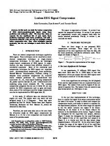
Figure 2.1: General components of a BCI system.
2.1
Brain Computer Interface Model and Architecture
The draft architecture of a BCI system can be summarized in Figure 2.1. A volitional control, a will to transmit information, is exerted by a user. A brain signal acquisition device captures her/his signals using a measurement modality. This module obtains the brainwaves and the information is digitalized and transmited to a computer device. Signal preprocessing is applied to eliminate nuisances and artifacts and to enhance the Signal to Noise Ratio (SNR), or to apply spatial or frequency filters. In the next step, a feature is carefully constructed in order to differentiate at least between two different mental states. Finally a classification step is applied to derive the actual information bit out of the system. An application system uses this information to affect some external device. By visual or any other sensory means, the feedback is fed back to the user and a loop is finally closed. The central point of this system is called the Brain Machine Dilemma [154]. The underlying idea is that the BCI system adapts to the user’s thinking patterns but, at the same time, the brain is adapting to what the system is doing, and changing their own signals in the process. This is the reason why it is often called, a co-adaptive system, where two different intelligent devices, one biological and the other electronic, try to adapt to each other.
9 Let X be a multichannel digital signal X ∈ RC×N , with N being the length of the digitalized signal in sample points, and C is the number of available channels. This signal matrix is
X(1, 1) · · · X(n, 1) · · · X(N, 1) .. .. .. . . . X = X(1, c) · · · X(n, c) · · · X(N, c) . .. .. .. . . . X(1, C) · · · X(n, C) · · · X(N, C)
(2.1)
The column x(n) of this matrix is a vector for a sample point index n in digital time for every available channel. Additionally, x(n, c) is a row with the multichannel signal as a scalar time-series for a particular channel c. When the particular channel is not important, the notation x(n) is used. The basic model of any BCI is to take this multichannel digital signal x(n), and transform it to an output control signal y(n) which can be a scalar or binary function. The BCI system can be modeled as the transformation T , which operates on the equation
y(n) = T [x(n)] .
(2.2)
What a BCI system must do, is to take at least a single bit of information out of y(n) and use that information to derive some action.
2.2
Signal Processing
From this signal processing point of view, BCIs are: • Causal: y(n) = T [x(m)], where m ≤ n. The action of a BCI system depends on the history of the captured brainwaves. • Dynamic: y(n) = T [x(m), x(m), ˙ x ¨(m), · · · ]. A BCI system is dynamic, where the output function does not depend only on the current value being observed, it does depend on its dynamic interactions. • Time invariant: y(n) = T [x(n)] ⇒ y(n − p) = T [x(n − p)]. The output of a BCI system does not depend on the particular time frame where it is being used. However, adaptive BCI, which adapts to the user behavior, is time variant.
10 • Nonlinear: a system is linear when T [a1 x(n) + a2 x(n)] = a1 T [x(n)] + a2 T [x(n)]. Due to brainwave complexity, BCI systems are not linear. • Multirate or broadband [89]: The energy of brainwave spectrum is not confined to a certain band, and almost all frequency channels may convey some information. There are several filters that can be applied to the system to eliminate artifacts, enhance the signal, and to ease the detection of the discriminative information. Static filters like square or logartihmic, were traditionally used in analog signal processing and are currently already embedded in the measuring device. Wiener and Kallman filters are usually applied to invasive techniques [58]. The filter, particularly when it is linear, can be viewed as the matrix M in:
y(n) = M T [x(n)]
(2.3)
Spatial filters are carefully adapted to the arrangement of sensors around or within the head and they emphasize the spatial structure of the information that is being captured. The head is divided in anatomical regions and electrode locations around the head are arranged according to neuroanatomical planes or axes (Figure 2.2). Spectral filters, on the other hand, consider brainwaves as digital signals, and perform different transformations based on the spectral information contained within the signal x(n). They can be combined and aggregated creating filter banks to enhance signal quality.
(a) Neuronal Planes
(b) Neuroanatomical regions of the brain.
Figure 2.2: Neuronal Planes regularly used in neuroscience research. In BCI they are used to understand electrode location and spatial filters.
11
2.3
The Forward and Inverse Model
Brainwaves are obtained via sensors. Each one of them captures only a part or a version of the information. However, whatever is actually happening inside the brain is recovered indirectly from the sensor space. From there, the information can be traced back to the real landscape where the information source is located, inside the source space. This is a regular problem found in engineering and it is not different in BCI. Calculating the signal on each a sensor from a projection of a known source of information from within the head is called The Forward Problem[104, 154] and doing the opposite, estimating the contributions of different sources to whatever activity is found on sensors is called The Inverse Problem. Although the latter is a complex ill-posed problem, it is more relevant in BCI because it allows to determine source origins that can be mapped more directly to cognitive activities. Particularly for noninvasive electrophysiological modalities, an additional problem makes things harder. Due to its electrical properties, the brain acts like conductive gel, and any signal that is generated inside the brain is irradiated to every direction and it can influence every sensor regardless of its position. This is called Volume conduction [91, 23] and can be visualized in Figure 2.3.
2.4
Brain Signals Measuring Techniques
The measuring technique determines the most important taxonomic differentiation in BCI, according to the methodology that is applied to extract the information from the CNS. All of them have been used so far for BCI applications. 1. EEG Electroencephalography: it is based on the electrical voltage detected by electrodes at the scalp. It is explained in detail in Section 2.5. 2. ECoG Electrocorticography: the electrodes are located below the skull and above the cortex, on the exposed region of the brain. Thus, a craniotomy is required. It offers a very high temporal resolution, broader bandwidth and much better spatial resolution than EEG. This modality has allowed very good performance in complex BCI schemes like speech synthesis from direct neural signals [59]. 3. MEG Magnetoencephalography: when active neurons generate electric currents, minuscule magnetic fields are generated. It is considered complementary to EEG and ECoG, due to the fact that it is sensitive to the firing of neurons aligned parallel to
12
Figure 2.3: A source signal with positive/negative polarity is generated in a very specific region of the brain but due to volume conduction their influence affects a widespread area of the scalp where sensors are located (Image of the brain from Swartz Center for Computational Neuroscience).
13 the scalp, which are hard to detect in EEG and ECoG. Although MEG equipment is bulky and room-size, recent advances [18] are aiming to develop portable and wearable versions. 4. PET Positron Emission Tomography: this radio nuclear measuring device, use a tracer molecule like fludeoxyglucose, which emits positrons. Positrons interacts with biological tissue generating photons in exact opposite directions. The tracer is spread around the body and the brain, and its concentration is higher in those areas where active neuron firing is being conducted which requires more glucose [90]. 5. fMRI functional Magnetic Resonance Imaging: this noninvasive, non-portable measuring technique, measures the so-called BOLD response: the Blood Oxygen LevelDependent contrast. This is based on the principle that firing neurons generate an imbalance of oxyhemoglobin and deoxyhemoglobin which can be detected on the magnetic resonator, with a very high spatial accuracy. 6. fNIRS functional Near Infra Red Spectroscopy: it also measures the concentration changes of oxy/deoxy-hemoglobin using light pulses of near-infrared wavelengths. The different types of hemoglobin molecules absorb these light frequencies at different rates. It is an indirect measure of brain activity. It is also portable and wearable. Although it provides very good spatial localization, temporal localization is hindered by the hemodynamic response [90]. 7. INR Intracortical Neuron Recordings: Electrodes, tetrodes, or Multielectrode Arrays, MEAs (i.e. Utah Array) [2], can be implanted inside the brain. Often called iEEG, intracraneal EEG, are designed to detect Local Field Potentials LFPs or even single-unit recording [23]. ECoG and INR are invasive technologies that require a neurosurgery or craniotomy. The implantation of electrodes is performed inside the skull for the former, and inside the brain for the latter. The remaining measuring techniques are external or noninvasive.
2.5
Electroencephalography
Above all, electroencephalography, is the most widespread method to gather information from the CNS in a non-invasive way. It is of particular interest in BCI mainly because of its non-invasiveness, its optimal time resolution and acceptable spatial resolution. Moreover,
14 it is portable, cheap, wearable and can be more easily integrated into fashionable designs aimed for real users, which prefer cap-like devices [63]. The electroencephalography consists on the measurement of small variations of electrical voltage over the scalp. This represents mainly the summed activity of Post-Synaptic Potentials (PSPs) of pyramidal neurons located perpendicular to the scalp [91]. Only one percent of synchronized activity of pyramidal neurons are stronger that the remaining desynchronized neurons [123] and explain ninety-nine percent of the signals obtained from EEG. This technique is one of the most widespread used methods to capture brain signals and was initially developed by Hans Berger in 1924 and has been extensively used for decades to diagnose neural diseases and other medical conditions. Figure 2.4 shows a sample EEG signal trace obtained with a digital and wearable EEG device. The first characterization that Dr. Berger detected was the Visual Cortical Alpha Wave, the Berger Rythm [66]. He understood that the amplitude and shape of this rhythm was coherently associated to a cognitive action (eyes closing). We should ask ourselves if the research advancement that came after that discovery would have happened if it weren’t so evident that the shape alteration was due to a very simple and verifiable cognitive process. The EEG signal is a highly complex multi-channel time-series. It can be modeled as a linear stochastic process with great similarities to noise [136]. It is measured in microvolts, and those slightly variations are contaminated with heavy endogenous artifacts and exogenous spurious signals. The device that captures these small variations in current potentials over the scalp is called the electroencephalograph (Figure 2.6). Electrodes are located in predetermined positions over the head, usually embedded in saline solutions to facilitate the electrophysiological interface and are connected to a differential amplifier with a high gain which allows the measurement of tiny signals. Although initially analog devices were developed and used, nowadays digital versions connected directly to a computer are pervasive. A detailed explanation on the particularities and modeling of EEG can be obtained from [64], and a description of its electrophysiological aspects from [55]. Further details are covered in Chapter 4.
2.6
EEG Signals
Overall, EEG signals can be described by their phase, amplitude, frequency and waveform. The following components regularly characterize EEG signals:
15
Ch.
Fz Cz P3 Pz P4 PO7 PO8 Oz Help
10 0
11 200
12 400
600
13 800
14 1000
15 1200
1400
Figure 2.4: Sample EEG signal obtained from Time (s) (g.Nautilus, g.Tec, Austria). Time axis is in seconds and five seconds are displayed. The eight channels provided by this device are shown.
Figure 2.5: International 10-20 system that standardize electrode locations over the scalp.
16
Figure 2.6: Digital and wearable electroencephalographs. • Artifacts: These are signal sources which are not generated from the CNS, but can be detected from the EEG signal. They are called endogeneous or physiological when they are generated from a biological source like ocular movements or from any other muscle, etc., and exogeneous or non-physiological when they have an external electromagnetic source like line induced currents or electromagnetic noise [152]. Ambulatory studies or out-of-the lab studies introduces artifacts that are derived from the person movement, from any kind of muscular electrical stimulator for rehabilitation treatments or from other devices in hybrid, or multi-modal BCIs. • Non-Stationarity: the statistical parameters that describe the EEG as a random process are not conserved through time, i.e. its mean and variance, and any other higher-order moments are not time-invariant [66]. • DC drift and trending: in EEG jargon, which is derived from concepts of electrical amplifiers theory, Direct Current (DC) refers to very low frequency components of the EEG signal which varies around a common center, usually the zero value. DC drift means that this center value drifts in time. Although sometimes considered as a nuisance that needs to get rid of, it is known that very important cognitive phenomena like slow cortical potentials or slow activity transients in infants do affect the drift and can be used to understand some particular brain functioning [146, 123]. • Basal EEG activity: the EEG is the compound summation of myriads of electrical sources from the CNS. These sources generate a baseline EEG which shows continuous activity with a small or null relation with any concurrent cognitive activity or task. • Intra-subject and Inter-subject variability: electroencephalographic signals vary from person to person. Additionally, EEG can be affected by the person’s behavior like
17 sleep hygiene, caffeine intake, smoking habit or alcohol intake previously to the signal measuring procedure [43]. Regarding how the EEG activity can be related to an external stimulus that is affecting the subject, it can be considered as • Spontaneous: activity related to basal EEG, arising spontaneously, or self-regulated by the person. • Evoked: activity that can be detected synchronously after some specific amount of time from the onset of the stimulus. This is usually referred as time-locked. In contrast to the previous one, it is often called induced activity. Additionally, according to the existence of a repeated rhythm, the EEG activity can be understood as • Rhythmic: EEG activity consisting of waves of approximately constant frequency. It is often abbreviated RA (regular or rythmic activity). They are loosely classified by their frequencies, and their naming convention was derived from the original naming used by Hans Berger himself: – Delta (0-4 Hz) – Theta (4-8 Hz) – Alpha Waves (10 Hz) – Sigma (12-16 Hz) – Beta (12-30 Hz) – Gamma (30-100 Hz) – Omega (60-120 Hz) – Rho (250 Hz) hippocampal – Sigma Thalamocortical burst (600 Hz) [45]. The last three are hardly encountered in conventional EEG [146]. • Arrhythmic: EEG activity in which no stable rhythms are present. • Dysrhythmic: Rhythms and/or patterns of EEG activity that characteristically appear in patient groups and rarely seen in healthy subjects.
18 The number of electrodes and their positions over the scalp determines a spatial structure: signal elements can be generalized, focal or lateralized, depending on in which channel (i.e. electrode) they are found.
2.7
BCI EEG Paradigms
BCI Paradigms are referred to noninvasive EEG-based BCI configurations that are used to transmit volitional information. The popularity of EEG in BCI Research influenced the adoption of conventional paradigms exclusively for noninvasive BCI. Their chronology can be found at the beginning of the Chapter. They can be roughly [27] described as: 1. Steady State Evoked Potentials: the basis for this paradigm is that when a subject attends certain stimulus, the dominant frequency component contained in the stimulus source can be found in the brain waves. When stimulus sources are light, this is called SS Visual EP and the signals are prominent in occipital regions. A similar process can be obtained with auditory stimulus, in which case they are called SS Auditory EPs. Finally, this can be extended to somatosensory stimulation (i.e. tactile) and it is called SS Somatosensory EP. By using different stimulus sources with different frequencies, the one that is selectively attended by a subject can be inferred based on the main frequency component found on the EEG trace [90]. 2. Bereitschaftspotentials, Readiness Potential or Movement-Related (Cortical) Potentials: these signals are low frequency [0.05, 3] Hz cortical potential that can appear when a subject is just about to engage in a movement related activity. They are used in BCI as triggering markers, or to identify movement-related EEG activity for neurorehabilitation [126]. 3. Motor Imagery ERD/ERS: the motor imagery, i.e. the mental visualization of movement without actually performing it, triggers a neurophysiological response which is very similar to the one obtained when the movement is physically performed. Frequencies on the α range of EEG are desynchronized prior to movement imagery, and synchronized afterwards. At the same time, β frequencies are resynchronized and increase in power after motor imagery. A subject can learn to think about moving a feet or moving a limb, and transfer an information bit from this thinking patterns. This paradigm requires intensive training from subjects. This is further explained in Chapter 6.
19 4. P300: the positive deflection at 300 ms is activated by a cognitive experiment called the oddball paradigm and can be used to detect which symbol a subject is paying attention on a flickering matrix. By exploiting this information, a speller application can be implemented. This important signal is explained in details in Chapter 7. 5. Mental Tasks: mentally rotating 3D objects, or calculating arithmetic operations are used to generate signals that can be detected and utilized to transfer an information bit [127]. 6. Slow Cortical Potentials: these are very slow shifts in the electrical activity found in the cortex, of a very low frequency. They can be modulated by operand conditioning protocols [154]. 7. Error Potentials: when a person recognizes that an error was committed during a task, a recognizable signal called ErrP can be detected along the EEG trace, time-locked to the onset when the error information is fed back to the person. This very important potential is used in BCI applications to enhance the identification of false positives and to improve the overall interaction between the subject and the computer [35]. 8. Visual Spatial Covert Attention: oscillatory activity in the α band of EEG can be modulated by changes in visual covert attention. Visual covert attention is the ability to focus attention on objects on the peripheral vision. Humans can voluntarily focus attention to locations in visual space without moving their eyes. This voluntary control is reflected in changes on Visual Occipital Alpha Waves [68]. Alpha Waves are further detailed in Chapter 5. These paradigms have been exploited in the most popular BCI configurations, the Wadsworth BCI, the Graz BCI, the Berlin BCI and the T¨ ubingen BCI. These platforms introduced pragmatic enhancements to use these paradigms to implement more practical devices [91, 123, 16, 106, 92, 148].
2.8
State of the Art of BCI Algorithms for EEG processing
According to the general layout of a BCI system, Figure 2.1, specific algorithms or techniques are required for both the feature extraction and classification step. The most relevant features used nowadays in BCI are:
20 • Time points: the sequence of time series, often, concatenated in time or space. • Band Power: frequency based features. • Complexity: based on complexity measurements like entropy, or fractal. • Statistical: Auto-regressive parameters or covariance matrices. The most successfull used and verified classification methods for BCI [82] can be described as linear versions of machine learning tools. Particularly, Support Vector Machines (SVM), Linear Discriminant Analysis (LDA) and its variant Stepwise Linear Discriminant Analysis (SWLDA) [76, 122]. SWLDA is relevant for two reasons: the first is that the stepwise dimension weighting improves the feature selection criteria and it also enhances the spatial filter that this procedure encompass. The second reason, from a pragmatic perspective, is that this method is included in the popular BCI2000 [121] package and is the default option for the identification of event related potentials. Spatial filters are also used and they show substantial improvements in classification accuracies: the canonical Common Spatial Patterns CSP [6] for the identification of Motor Imagery as well as the xDAWN [117] algorithm for P300 identification. In recent years (circa 2018) classification accuracies in BCI have improved but the focus was not centered on any particular classification algorithm. Instead, current contributions concentrate their efforts on how these algoritms are used [81]. Recent works can be described as: • Ensemble classifiers: SVM ensembles [109] and variants of random forest [131]. Features are segmented and divided and the forest performs a classification step on aggregated parts, maximizing classification accuracies. • Cross-paradigm BCI: the use of a reinforced signal with ErrP feedback or the use of SSVEP in combination with P300 detection [81]. • Adaptive classifiers: the parameters of the classifiers are adapted continuously and online, adapting to the natural variation of the EEG signals [81]. • Transfer learning: transfer the calibration information obtained by users to new subjects. This aims to ease the issue of the inter-subject variability in BCI, and to reduce the set-up and calibration times of a BCI system [160].
21 • Rienmann geometry classifiers: the EEG stream is directly mapped onto a geometrical space equipped with a suitable Riemannian metric. Hence, further data manipulation is carried out following principles of Riemannian geometry which yields very good results in terms of accuracies [160]. • Tensor-based BCI: the EEG data is viewed as a multidimensional matrix, a tensor. The BCI operation is considered as an optimization problem that can be solved with sparsity and nonnegativity constraints [150, 29]. • Deep learning: deep learning is a very successful technique driven by the increased computational power of current computer devices. Deep learning techniques have also being applied to BCI applications [139].
2.9
EEG Waveform Analysis
This section describes the depictions that are used to describe EEG signals waveforms and the automatic procedures that were developed with this purpose. 2.9.1
EEG Waveform Characterization
The shape of the signal, the waveform, can be defined as the graphed line that represents the signal’s amplitude plotted against time. It can also be called EEG biomarker, EEG pattern, motifs, signal shape, signal form and a morphological signal [66]. The signal context is crucial for waveform characterization, both in a spatial and in a temporal domain [66]. Depending on the context, some specific waveform can be considered as noise while in other cases is precisely the element which has a cognitive functional implication. A waveform can have a characteristic shape, a rising or falling phase, a pronounced plateau or it may be composed of ripples and wiggles. In order to describe them, they are characterized by its amplitude, the arch, whether they have (non)sinusoidal shape, by the presence of an oscillation or imitating a sawtooth (e.g. Motor Cortical Beta Oscillations). The characterization by their sharpness is also common, particularly in Epilepsy, and they can also be identified by their resemblance to spikes (e.g. Spike-wave discharge). Other depictions may include, subjective definitions of sharper, arch comb or wicket shape, rectangular, containing a decay phase or voltage rise, peaks and troughs, short term voltage change around each extrema in the raw trace. Derived ratios and indexes can be used
22 as well, like peak and trough sharpness ratio, symmetry between rise and decay phase and slope ratio (steepness of the rise period to that of the adjacent decay period). For instance, wording like ”Central trough is sharper and more negative that the adjacent troughs” are common in the literature. Other regular characterizations which are based on shape features may include: • Attenuation: Also called suppression or depression. Reduction of amplitude of EEG activity resulting from decreased voltage. When activity is attenuated by stimulation, it is said to have been ”blocked” or to show ”blocking”. • Hypersynchrony: Seen as an increase in voltage and regularity of rhythmic activity, or within the alpha, beta, or theta range. The term suggests an increase in the number of neural elements contributing to the rhythm and a synchronization of neurons with similar firing patterns [23]. • Paroxysmal: Activity that emerges from background with a rapid onset, reaching (usually) quite high voltage and ending with an abrupt return to lower voltage activity. • Monomorphic: Distinct EEG activity appearing to be composed of one dominant activity. • Polymorphic: Distinct EEG activity composed of multiple frequencies that combine to form a complex waveform. • Transient/Component: An isolated wave or pattern that is distinctly different from background activity. The conventional clinical procedure consists in analyzing the paper strip that is generated by the plot of the signal obtained from the device. Expert technician and physicians analyze visually the plots looking for specific patterns that may give a hint of the underlying cognitive process or pathology. Atlases and guidelines were created in order to help in the recognition of these complex patterns. Even video-electroencephalography scalp recordings are routinely used as a diagnostic tools [48]. The clinical EEG research has coined a term for the graphical depictions of EEG waves: graphoelements, and a whole branch of electrophenomenology has arisen around them [123]. Sleep research has been studied in this way by performing Polysomnographic recordings (PSG) [118], where the different sleep stages are evaluated by visually marking waveforms
23 or graphoelements in long-running electroencephalographic recordings, looking for patterns based on standardized guidelines. Visual characterization includes the identification or classification of certain waveform components, or transient events, based on a subjective characterization (e.g. positive or negative peak polarity) or the location within the strip. It is regular to establish an amplitude difference between different waveforms from which a relation between them is established and a structured index is created (e.g. sleep K-Complex is well characterized based on rates between positive vs. negative amplitude) [140]. Other relevant EEG patterns for sleep stage scoring are alpha, theta, and delta waves, sleep spindles, polysplindles, Vertex Sharp Waves (VSW), and sawtooth waves (REM Sleep). Moreover, EEG data acquisition is a key procedure during the assessment of patients with focal epilepsy for potential seizure surgery, where the source of the seizure activity must be reliably identified. The onset of the epileptic seizure is defined as the first electrical change seen in the EEG rhythm which can be visually identified from the context and it is verified against any clinical sign indicating seizure onset. The Interictal Epileptiform Discharges (IEDs) are visually identified from the paper strip, and they are also named according to their shape: spike, spike and wave or sharp-wave discharges[21].
2.9.2
EEG Waveform Analysis Algorithms
Shape or waveform analysis methods are considered as nonparametric methods. They explore signal’s time-domain metrics or even derive more complex indexes or features from it [137]. One of the earliest approach to automatically process EEG data is the Peak Picking method. Although of limited usability, this procedure has been used to determine latency of transient events in EEG [67, 161]. Straightforward in its implementation, it consists in selecting a simple component based on the expected location of its more prominent deflection [101]. Evoked Potentials (EPs) and Event Related Potentials (ERPs) are transient component that may arise as a brain response to an external visual, tactile or auditory stimulus. Auditory EPs are regularly used clinically to assess auditory response in infants. Particularly, the P300 signal that is used for some BCI Spellers is a prototypical Event Related Potential. ERPs are characterized by their most prominent peaks, where the name of many of the EEG features evoke directly a peak within the component, e.g. P300 or P3a, P3b or N100. This leads to a natural procedure to classify them visually by selecting appropriate peaks and matching their positions and amplitudes in an orderly manner. The letter provides the polarity (Positive or Negative) and the numbering shows the time
24 referencing the stimulus onset, or the ordinal position of each peak (first, second, etc). Finally, the trailing letter is added to describe different variants of components that initially were considered the same. A related method is used in [5] where the area under the curve of the EEG is sumarized to derive a feature. This was used in the seminal work of Farwell and Donchin on P300 [42, 154]. Additionally, a logarithmic graph of the peak-to-peak amplitude which is called amplitude integrated EEG (aEEG) [125] is utilized nowadays in Neonatal Intensive Care Units (NICU). Other works explored the idea to extend human capacities analyzing EEG waveforms [74] where a feature from the amplitude and frequency of its signal and its derivative in time-domain is used. Moreover, alternative schemes explored the use of Mathematical Morphology, where the time-domain structure of contractions and dilations are studied [155]. The Merging of Increasing and Decreasing Sequences (MIDS) [162] provides a filter or heterogeneous downsampling scheme which is based on the waveform structure, similar to what is provided in Local Binary Patterns (1-D LNBP, 1D-LBP and LBP) algorithms [65]. Finally the proposals of Burch, Fujimori, Uchida and the Period Amplitude Analysis (PAA) algorithm are few of the earliest algorithms where the idea of capturing the shape of the signal were established [141]. Three algorithms are explained in detail in the following section.
2.9.3
Waveform-based Feature Extraction Algorithms
The method presented in this Thesis generates a feature that can be classified. Likewise, the following methods provide a feature that can be used as a template, whereas all of them are based on metrics extracted from the shape of the signal. These features can be used to create dictionaries or template databases. These templates provide the basis for the pattern matching algorithm and offline classification. The notation f = {fi }n1 or f = {fi }i∈J is utilized to describe the concatenation of scalar values to form a multidimensional feature vector f = {f1 , f2 , ..., fn }, while x(n) is used as a single-channel EEG time series for a given fixed channel.
Matching Pursuit - MP 1 and MP 2 Pursuit algorithms refer, in their many variants, as blind source separation [150] techniques that assume the EEG signal as a linear combination of different sparse sources extracted
25 from a template’s dictionaries. Matching Pursuit MP [87], the most representative of these algorithms, is a greedy variant that decomposes a signal into a linear combination of waveforms, called atoms, that are well localized in time and frequency [26]. Given a signal, this optimization technique, tries to find the indexes of m atoms and their weights (contributions) that minimize,
m
X
ε = x(n) − wi gi (n)
(2.4)
i=1
which is the error between the signal and its approximation constructed by the weighted wi atoms gi , and calculating the euclidean norm k·k2 . The algorithm goes by first setting the approximating signal x ˜0 as the original signal itself, x ˜0 (n) = x(n)
(2.5)
and setting the iterative counter s as 1. Hence, it searches recurrently the best template out of the dictionary that matches current approximation. N X gs = arg max x ˜s−1 (n) gi (n) gi
(2.6)
n=1
where gi are all the available scaled, translated and modulated atoms from the dictionary. The operation |·| corresponds to the absolute value of the inner product. This step determines the atom selection process, and their contribution is calculated based on PN ws =
˜s−1 (n) n=1 x kgs k2
gs (n)
(2.7)
with s representing the index of the selected atom gs and k·k its euclidean norm. Finally the contribution of each atom is subtracted from the next approximation [32, 120, 87]
x ˜s (n) = x ˜s−1 (n) − ws gs (n)
(2.8)
The stopping criteria can be established based on a limiting threshold on Equation 2.4 or based on a predetermined number of steps and selected atoms. Two variants of this algorithm are evaluated. In MP 1 the dictionary is constructed with the normalized templates directly extracted from the real signal segments which is a straightforward implementation of the pattern matching technique. In MP 2 the coefficients of Daubechies least-asymetric wavelet with 2 vanishing moments atoms are used to construct the dictionary [147]. For the first
26 version, the matching against the template is evaluated according to Equation 2.4 directly, whereas for the latter each feature is crafted by decomposing the signal in its coefficients and building, an eventually sparse, vector with them: �D
� f=
wi
(2.9) 1
where D is the size of the dictionary.
Permutation Entropy - PE Bandt and Pompe Permutation Entropy has been extensively used in EEG processing, with applications on anesthesia, sleep stage evaluation and increasingly for Epilepsy pre-ictal detection [11]. This method generates a code based on the orderly arrangement of sequential samples, and then derives a metric which is based on the number of times each sequence is found along the signal. This numeric value can be calculated as information entropy [93]. Let’s consider a signal on a window of length W represented by the sample points
(x1 , x2 , ..., xW )
(2.10)
and resampled by τ intervals, starting from the sampling point n, doing
(xn , xn+τ , xn+2τ ..., xn+(m−1)τ ).
(2.11)
This sequence is of order m, which is the number of sample points used to derive the ordinal element called π. There are m! ways in which this sequence can be orderly arranged, according to the position that each sample point holds within the sequence in a decreasing order relationship. For example if m = 3, and the first sample point is the bigger, the second is the smaller and the third one is in the middle, the ordinal element π corresponds to (1, 3, 2). Thus, along the signal window there can be at most k different ordinal (and overlapping) elements πs
(π1 , π2 , ..., πk )
(2.12)
with k = W −(m−1)τ . The probability density function pdf for all the available permutations P of order m should be p = (p1 , p2 , ..., pm! ) with m! i=1 pi = 1.
27 Hence, the time series window is mapped to a new set of k ordinal elements, and the pdf can be calculated by the empirical permutation entropy,
pi =
k 1X [πs = πi ] k
(2.13)
s=1
with 1 ≤ i ≤ m!. The Iverson Bracket [·] resolves to 1 when their logical proposition argument is true, 0 otherwise. Therefore, for each i only those ordinal elements πs that were effectively found along the signal are counted to estimate pi , and zero elsewhere. The empirical permutation entropy can be calculated from the histogram as,
H(p) =
m! X
pi log
i=1
1 . pi
(2.14)
An efficient implementation can be derived from [142], and the model description is based on [14]. This procedure produces a scalar number for the given signal window of size W . To derive a feature, a sliding window procedure must be implemented to cover an entire segment of length N . Thus, the length of the feature is N − (W + τ (m − 1)). � �N f = H(p)u
.
(2.15)
W +τ m
with u varying on a sample by sample basis along the signal, starting from the specified index. Slope Horizontal Chain Code - SHCC This algorithm [5] proceeds by generating a coding scheme from a sequence of sample points. This encoding is based on the angle between the horizontal line on a 2D-plane and any segment produced by two consecutive sample points, regarding them as coordinates on that plane. A signal of length N , can be represented by a list of ordered-pairs e,
e = [(x, y)1 , (x, y)2 , ..., (x, y)N ]
(2.16)
and it can be divided into G different blocks. These blocks are obtained by resampling the original signal from the index
G = bn + (m∆) + 0.5c
(2.17)
28 with n being the original sampling index on 1 ≤ n ≤ N and b·c being the floor operation, i.e. rounding of the number argument to the closest smaller integer number. On the other hand, ∆ can be obtained by �
N ∆= G+1
� (2.18)
with G < N and using instead d·e as the ceil operation, the rounding to the closest bigger integer number. Lastly, the value m can be derived from � �� � N − 1 N −1 m = sign ∆ . ∆
(2.19)
This resampling produces a new sequence of values, � � e0 = (x0 , y 0 )1 , ..., (x0 , y 0 )s , ..., (x0 , y 0 )G .
(2.20)
The next step is the normalization of each ordered-pair as vectors x’ = (x01 , ..., x0G ) and 0 ) according to y’ = (y10 , ..., yG
ˆ= x
x’ − min(x’)1 max(x’) − min(x’)
(2.21)
ˆ= y
y’ − min(y’)1 max(y’) − min(y’)
(2.22)
with 1 being the vector of length G with all their components equal to 1. Hence, the scalar ˆ , and yˆs of y ˆ , with s varying between 1 and G are effectively normalized components x ˆs of x to x ˆs , yˆs ∈ [0, 1]. Finally, the feature is constructed by calculating the point-to-point slope against the horizontal plane, � f=
yˆs − yˆs−1 x ˆs − x ˆs−1
�G (2.23) 2
Chapter 3
From signals to images A regular practice in image processing is to analyze images as bidimensional signals. In this Thesis the opposite is done and signals are studied by how they are represented on images. This chapter describes the procedure to plot an image from the digital EEG signal. This image is used to extract features which represents the waveform, the structure of the signal on a plot. By analyzing these features, we hypothesize that the underlying cognitive process can be detected and it can be used to implement a brain-computer communication device.
3.1
Electroencephalographic Plotting
The plotting of the EEG is intrinsically mixed with the nuisances of the electroencephalography itself. Plotting proceed by using a chart recorded with a single pen [69]. Voltages are represented on a vertical axis while time is represented on the horizontal axis, in a Cartesian arrangement. The most salient characteristics of a plot are: 1. Sensitivity: also termed gain due the amplification procedure. Its units are the digital form, it is
mV mm .
In
µV pixel .
2. Epoch/Paper speed: the time span that is represented in a single screen. For paper strips it is usually 10s. In its digital counterpart is
w pixel
with w being the length in
seconds of the signal segment. Additionally, on analog plotting montage is essential, while digital plotting allows flexible montage configuration from software. Montage can be monopolar or bipolar. On monopolar montages each electrode obtains the potential difference against a common reference. With bipolar montages, electrodes are paired, eventually in chained configurations, and the potential difference is obtained between each pair of electrodes [21]. 29
30 Neuroimaging With the advent of digital computers and the digital revolution, plotting has became imaging. Medical imaging is defined as the making of a visual representation of an organ with a detector or sensor. However, the concept has extended and brain imaging modalities is synonym of brain measuring devices. Neuroimaging [46] entails image mapping activity or structure to neuroanatomical regions. There are currently three categories of neuroimaging: structural which includes Computed Tomography (CT), Magnetic Resonance Imaging (MRI) and Diffusion Tensor Imaging (DTI), functional, which encompass EEG, MEG, fMRI, PET, Single Positron Emission Computed Tomography (SPECT), NIRS and chemical which involves special dyes which are sensible to neuron firing. Indeed, analyzing image plots is a form of brain imaging.
3.2
Signal to Image transformation
The EEG signal is represented by
x(n, c)
(3.1)
where n is the index of sample points digitalized at sampling frequency Fs . This is a multichannel signal, for c varying between 1 ≤ c ≤ C. Each one of this channels is assigned a name according to the 10-20 international system (see Figure 2.5), and there are C available channels. The sample index n varies between 1 and N . The span of the signal λ is the length in milliseconds of the waveform under study. The length of segment N in sample point units, the sampling frequency Fs in Hz and the segment length w in seconds are related by N = bFs wc .
(3.2)
Additionally the signal can be scaled on amplitude by the scale factor γ or in time by the time scale factor γt . The γt parameter can also be used to convert from time to sample point index by doing n = bFs tc γt .
(3.3)
To extract features from an image, it should be first constructed. The straightforward way to do it, replicating the analog or digital EEG plotting, is to draw a line on a contrast
31
Figure 3.1: Sample EEG signal plot. For this sample image, the length of the signal is 1s, which is 250 sample points. The height of the image is 73 pixels, which is the peak-to-peak amplitude of the signal segment. Channel Oz of baseline EEG activity is being shown. background. This line represents the voltage amplitude of a channel c in relation to a reference zero-level z(c), with a positive deflection going upwards and downwards for negative deflection. Figure 3.1 shows an example of an EEG signal segment plot. This image is a black-and-white binary image. The color selection is arbitrary (white for the line, black for the background), but it has some implications in terms of the feature extraction procedure that will described in Section 4.2. This chapter mostly deals with the coordinates transformation that need to be enforced while converting the signal into a plot. Figure 3.2 shows the image coordinate system where the (z1 , z2 ), with z1 , z2 ∈ N0 × N0 , represent the horizontal and vertical locations, and the (0, 0) value is the upper-left position of the image. Let ci be a given constant channel, the values of I(z1 , z2 ) are obtained for n varying between 1 and N or c varying between 1 and C. In order to convert the EEG original signal x(n, c) into a time-domain image I(z1 , z2 ) representation, the following alternatives can be used: 1. Channel-by-channel binary image: The standard plotting, on a black-and-white image with lines representing voltage amplitude: 255 if z = n; z = x(n, c ) + z(c ) 1 2 i i I (ci ) (z1 , z2 ) = . 0 otherwise
(3.4)
Due to the coordinates transformation, the signal plotted by this procedure is inverted on the image. Thus, it is necessary to multiply x(n, ci ) by (−1) to invert it before plotting.
32
+
(0,0) +
(Wx , Hy ) Figure 3.2: The image coordinate system and the mapping from the signal segment. The origin is the (0, 0) position at the upper-left corner of the image. Time is represented as sample points on the horizontal axis, and the amplitude in µV is shown on the vertical axis. Image height Hy and width Wx are obtained based on signal parameters. The signal’s zero-level z(c) is the vertical location where the signal zero value is located. The plot of the signal is obtained by first setting the sample points on the predetermined image locations according to equation 3.15 and then applying a discrete interpolation algorithm to connect them with straight lines. The plotted waveform is a K-Complex.
2. Multichannel full greyscale image The image is greyscale. Voltage amplitudes are represented by the pixel content and each channel is represented on the vertical axis. The height of the signal is equal to the number of channels. This is used in Neuroimaging [46] plots of ERP events:
I(z1 , z2 ) =
n
φ(x(n, c)) if z1 = n; z2 = c .
(3.5)
3. Multichannel stationary binary image: The horizontal axis of the image is not time, but it is the number of the channel instead. In this representation different contributions from different channels can be
33 explored at the same time, but time dynamics is lost.
255 if z = c; z = x(n , c) + Z 1 2 i I (ni ) (z1 , z2 ) = . 0 otherwise
(3.6)
In this case, the vertical position where the signal’s zero value is located in Z. 4. Multichannel stationary greyscale image This is a variant of the previous one, where the horizontal axis also represent the channel. In this form, the intensity of the contribution of each channel is represented by the greyscale pixel value. Combined with head models and forward projection solutions this is the methodology used to represent scalp heatmaps [50]:
φ(x(n , c)) if z = c; z = Z i 1 2 I (ni ) (z1 , z2 ) = . 0 otherwise
(3.7)
5. Channel by channel full greyscale image This is similar to a raster plot [32] but the greyscale image representing voltages in pixel intensities can be replicated or epoched H times, which at the same time is the height of the image. The selection of this value depends on the number of epochs or repetitions to show. In this case, the mapping is
I (ci ) (z1 , z2 ) =
n
φ(x(n, ci )) if z1 = n; z2 = H .
(3.8)
To analyze effectively an EEG signal, many signal segments must be produced. Hence, the transformation from signal to image is continuously repeated, and many images need to be crafted for the EEG signal under analysis. How to determine the size of all the images so that they can be effectively compared between them ? The first option is to regularize the signal and fit in an equal size for every image. An alternative choice is to autoscale every image according to the zero-level position. Figure 3.3 shows two sample artificial impulse signals and their alternative transformation into images.
34
3.3
Standardized plotting
The z-score is a widely used method to regularize a signal [143, 162]. This standardization procedure is defined for 1 ≤ n ≤ N and 1 ≤ c ≤ C by doing
x ˜(n, c) =
x(n, c) − x ¯(c) σ ˆ (c)
(3.9)
where x(n, c) is the multichannel EEG signal segment for the sample point index n and for channel c. The values x ¯(c) =
N 1 X x(n, c) N n=1
and � σ ˆ (c) =
N
1 X [x(n, c) − x ¯(c)]2 N −1
�1 2
n=1
are the mean and estimated standard deviation of x(n, c), 1 ≤ n ≤ N , for each channel c. Figure 3.3(a) shows an impulse signal and their standardized representation.
3.4
Autoscaled plotting
This plotting scheme allows each image to adapt to the underlying signal. The signal is centered [143] while the image height is autoscaled. The height is set at twice the value of the zero-level, and the signal mean is subtracted from the original signal, producing a vertical displacement, according to the following Equation, x ˜(n, c) = x(n, c) − x ¯(c)
(3.10)
Figure 3.3(b) shows the results of the plotting for an impulse signal. Equation 3.10 has the advantage that any low frequency component, particularly the EEG DC drift is eliminated, due to the fact that plot of the signal is always centered on each image.
3.5
Zero-Level
The zero-level z(c) is the image vertical position where the signal’s zero value has to be situated in order to fit the entire signal within the image for each channel c:
�
� � � maxn x ˜(n, c) − minn x ˜(n, c) maxn x ˜(n, c) + minn x ˜(n, c) z(c) = − 2 2
(3.11)
35
(a) Standardized: The signal is standardized and the height of the image is determined according to the peak-to-peak amplitude, which is similar for every image.
(b) Autoscaled: The plotted image height is twice the zero-level, which is also determined according to the peak-to-peak amplitude of each segment, proportional to γ, and not constant. Transformed images do not have the same height, but the zero-level is always located at half the height of the image.
Figure 3.3: An artificial signal pulse and its plotting representations.
j k z(c) = min x ˜(n, c) n
where the minimization and maximization are carried out for n varying between 1 ≤ n ≤ N . The result of Equation 3.11 is the length of the positive peak of the signal because the signal is inverted before the plot is constructed. This value represents the vertical location on the image where the signal goes to zero.
3.6
Image Size
Height The height of the image is calculated according to the peak-to-peak amplitude of the signal segment, and proportional to the amplitude scale factor γ:
Hy = max bγ x ˜(n, c)e − min bγ x ˜(n, c)e
(3.12)
while for the autoscalable version, it is just twice the value of the zero-level:
Hy = 2 z(c).
(3.13)
36 Width The width, on the other hand, is obtained based on the length of the signal segment, scaled by the γt scale time factor,
Wx = γt N
3.7
(3.14)
EEG Signal Plot
Once the regularization procedure, the size and the scale of the image are defined, a binary image I (c) can be constructed from a variant of the method specified in Equation 3.4 according to 255 if z = γ n 1 t I (c) (z1 , z2 ) = 0 otherwise
and z2 = bγ x ˜(n, c)e + z(c)
(3.15)
where 1 ≤ c ≤ C and 1 ≤ n ≤ N . The amplitude scale factor γ and time scale factor γt are used to determine the image size and at the same time the image resolution. This scheme produces a black-and-white plot of the signal with 255 being white and 0 black. There is one image per channel per segment.
3.8
Interpolation
Equation 3.15 produces a set of isolated pixels over the image I (c) . To produce the plot I (c) , the Bresenham [20, 111] algorithm is used to digitally interpolate straight lines between each pair of consecutive pixels. Figure 3.4(a) shows an image plot constructed by only using the sample points, while 3.4(b) shows the digital interpolation produced by the Bresenham algorithm. On Figure 3.4(c) the same signal can be observed produced when the time scaling factor γt is increased to 4. It can be noticed that there are very sharp edges around sample pixels. This can lead to a quantization of histogram gradients that will be discussed in the next Chapter. To reduce this sharpness of the signal on the plot, an alternative procedure is to use a smoothing interpolation of the signal x ˜(n, c) using splines. Instead of just situating time point values at a bigger step according to Equation 3.15, intermediate values are computed according to a linear, quadratic or cubic interpolation, hence smoothing the curve around each point. The result of this interpolation can be seen on Figure 3.4(d), where the edges
37
(a) Sample points are located on the image according to Equation 3.15.
(b) Sample points are linearly interpolated in a discrete procedure using the Bresenham algorithm.
(c) The digital signal is scaled 4 times (γt = 4) and the generated sample points are interpolated using the Bresenham algorithm.
(d) The digital signal is upsampled 4 times with a linear interpolation with splines. The Bresenham algorithm is used to perform the final digital interpolation to compose the plot.
Figure 3.4: Generated images based on different interpolation schemes.
38 around each sample point are more rounded. This procedure is similar to what the Matlab’s resample function does which also includes an antialiasing FIR lowpass filter [100]. Special care must be taken by the presence of artifacts around the signal endpoints, at the edges of the image. Those regions are excluded from further analysis. 30 20
Voltage [microV]
10 0 -10 -20 -30 -40 -50
0
50
100
150
200
250
Digital Time
(a) Vertical axis is voltage in µV while horizontal axis is expressed in sample points units.
(b) An image generated by the plotting algorithm for the same signal. Image height is 76 pixels, while width is 250. The zero-level z(c) value is 32.
Figure 3.5: One-second length basal EEG signal and the generated image, with Fs = 250.
3.9
Resolution and Precision
Image creation and signal plotting is a digitalization process [123]. Figure 3.5 shows an EEG signal and their plot representation. Any digitalization process is defined by their resolution, precision and dynamic range. The resolution [32] of the image transformation can be determined based on the characteristics of the digital signal and the parameter selection. On the horizontal axis of the image, one pixel is equivalent to
1Px ≡
1 [s] Fs γt
(3.16)
where Fs is the sampling frequency in Hertz, and γt is the time scale factor. This gives a value in seconds. For example, for Figure 3.1 where the length is 1s, the sampling frequency is 250Hz, and γt = 1, this gives a resolution of 1Px ≡ 0.0040s. Table 3.1 shows some reference values.
39 Table 3.1: Reference values for horizontal resolution γt
1Px
1 2 3 10 100
1 Fs s 1 1 2 Fs s 1 1 3 Fs s 1 1 10 Fs s 1 1 100 Fs s
1
Consistently, on the vertical axis, one pixel is analogous to
1Py ≡
1 [µV ] γ
(3.17)
where γ is the amplitude scale factor. As EEG time-series are digitalized in µV , this is the unit of choice. In Figure 3.1, 1 vertical pixel represents exactly 1µV . It is important to notice that the minimum recommended resolution for an EEG device is around 0.5 µV , which is an acceptable and practical level to detect physiological meaningful signals [123]. This level can be reached when γ is equal to 2. See Table 3.2 to see some reference values. Table 3.2: Reference values for vertical precision and resolution γ
1Py
Decimal Precision
1 2 3 10 100
1µV 1 2 µV 1 3 µV 1 10 µV 1 100 µV
0 0.5 0.3 0.1 0.01
Regarding the precision, discrete EEG time-series are floating-point numbers and the image is constructed based on discrete and integer pixels. Image’s pixel values (z1 , z2 ) are obtained according to Equation 3.15. Thus, on the horizontal axis z1 , no discretization is needed because time is already digitalized in sample units. Hence, there is no loss of precision in time from the one generated by the digital device where pixel values are obtained with
z1 = γt n,
(3.18)
where n refers to the sample point index. The maximum frequency that can be captured by the plotting scheme is half the number of pixels per seconds [123]. Equation 3.18 determines
40 at least a 1-to-1 relationship between pixels and sample points, thus the effective maximum frequency is only constrained by the Nyquist Frequency [100]. On the other hand, on the vertical axis, pixels are discretized according to z2 = bγ x ˜(n, c)e
(3.19)
where γ is the amplitude scale factor parameter, which also affects the height of the image in Equation 3.12. A rounding operation b·e is applied to obtain an integer representation. This means that precision is lost on the voltage amplitude. Table 3.2 shows some decimal precision values for different γ. Finally, the dynamic range of the digital capturing device is reduced to what is actually needed for each segment, because the height of the image is adjusted dynamically to the peak-to-peak amplitude, regardless of the plotting scheme.
Chapter 4
The Histogram of Gradient Orientations of Signal Plots This Chapter introduces the EEG feature extraction procedure based on the Histogram of Gradient Orientations. This method is grounded on an extension and modification of the SIFT [84] Descriptor which is used in Computer Vision to extract and map local regions of an image. At the same time, this Chapter brings to completion the previous one, describing how to mine the information from a plot and build a feature out of it.
4.1
Introduction
The work of Edelman, Intrator and Poggio [41] on how the visual cortex sense features was the inspiration to the development of an algorithm to identify and decode salient local information from image regions. The Scale Invariant Feature Transform (SIFT) method is composed of two parts, the SIFT Detector and the SIFT Descriptor. The first is the procedure to identify relevant areas of an image. The second is the procedure to describe and characterize a region of an image (patch) using the Histogram of Gradient Orientations 1 . The SIFT algorithm is biomimetically inspired in how the visual cortex detects shapes by analyzing orientations [78]. The patch description is also based on the Theory of Receptive Fields and other related ideas [79].
1 It should not to be confused with HOG [37], the Histogram Of Gradients which is another method from Computer Vision based on similar ideas. Actually, the descriptor part of the SIFT Method has no specific name, but it is based on building a histogram of gradient orientations.
41
42
4.2
Feature Extraction: Histogram of Gradient Orientations
The basic procedure is composed of, 1. Keypoints kp are located on an image of a signal plot. 2. A region of an image, a patch, is established using keypoints as centers. Each patch has a horizontal St and vertical scale Sv , which determines the size in pixels Sx and Sy , along the horizontal and vertical axis respectively. 3. From each patch, a descriptor d is derived which is used as a representation of the graphical information contained within the patch. On the image generated by the procedure detailed in previous Chapter, a keypoint kp is placed on a pixel (xkp , ykp ) over the image plot and a window around the keypoint is considered. A local image patch of size Sx × Sy pixels is constructed by dividing the window in 16 blocks. It is arranged in a 4 × 4 grid and the pixel kp is the patch center. Figure 4.1(a) shows a plot of a signal, a keypoint in red at the center and the surrounding patch. Pixel intensity gradients can be obtained from an image by applying the Sobel filter [135] and using finite differences to obtain pixel differences on the x and y direction. Composing them as vectors, oriented gradients on each pixel can be calculated. Figure 4.1(b) and (c) show vector field of oriented gradients. A local representation of the signal shape within the patch can be described by obtaining the gradient orientations on each of the 16 blocks and creating a histogram of gradients. In order to calculate the histogram, the interval [0 − 360] of possible angles is divided in 8 bins, each one at 45 degrees. Figure 4.1(d) shows a sample histogram obtained for eight orientations. Hence, for each spatial bin i, j = {0, 1, 2, 3}, corresponding to the indexes of each block Bi,j , the orientations are accumulated in a 3-dimensional histogram h through the following equation:
h(θ, i, j) =
X
ωang (∠J(p) − θ) ωij (p − kp) kJ(p)k
(4.1)
p
where p is a pixel from within the patch, θ is the angle bin with θ ∈ {0, 45, 90, 135, 180, 225, 270, 315}, kJ(p)k is the norm of the gradient vector in the pixel p, computed using finite differences, and ∠J(p) is the angle of the gradient vector. The scalar ωang (·) and vector ωij (·) functions
43 are linear interpolations used by [84] and [149] to provide a weighting contribution to eight adjacent bins. They are calculated as � � � 5 vy 5 vx ωij (v) = ω − xi ω − yi ∆s St ∆s Sv �
ωang (α) =
1 X r=−1
�
8α ω + 8r 2π
(4.2)
� (4.3)
where xi and yi are the spatial bin centers located in xi , yi ∈ {− 32 , − 21 , 12 , 23 }. The function parameter v = (vx , vy ) is a vector variable and α a scalar variable. The value of ∆s is the unit length of the patch, which is described in the section 4.4. On the other hand, r is an integer that can vary freely in the set {−1, 0, 1} and allows the argument α to be unconstrained in terms of its values in radians. The interpolating function ω(·) is defined as:
ω(z) = max(0, |z| − 1).
(4.4)
These binning functions conform a trilinear interpolation that has a combined effect of sharing the contribution of each oriented gradient between their eight adjacent bins in a tridimensional cube in the histogram space, and zero everywhere else. This procedure is important to avoid quantization issues that may appear with the histogram (i.e. elimination of intermediate values). Lastly, on Equation 4.2 the values of
5 ∆s S t
and
5 ∆s Sv
allow a unit conversion from pixel
to units-of-patch. As the patch has 16 blocks and 8 bin angles are considered, a feature d called descriptor of 128 dimension is obtained. This technique is a modification of Lowe’s SIFT Descriptor method. In Figure 4.2 the possible orientations on each patch are illustrated. The first eight orientations of the first block B1,1 , are labeled from 1 to 8 clockwise. The orientations of the second block B1,2 are labeled from 9 to 16. This labeling continues left-to-right, up-down until the eight orientations for all the sixteen blocks are assigned. They form the corresponding kp-descriptor of 128 coordinates.
4.3
Keypoint Location
The keypoint kp location must be accurately specified in order to establish the region from the signal where the waveform is located.
44
(b) A Sobel filter is applied to the image and a vector field of oriented gradients is calculated for each pixel.
Number of weighted gradients
(a) Example of a plot of the signal, a keypoint and the corresponding patch.
0
45
90
135
180
225
270
315
Bin Angles
(c) Zoomed-in vector field of oriented gradients around the signal plot. Each pixel is assigned an orientation and magnitude.
(d) Eight oriented bins are used on each block to identify the oriented gradients within each block.
Figure 4.1: Patch and vector field of oriented gradients. . For the horizontal position, the localization of the keypoint is based on a priori information, based on the characteristics of the event under study. For instance, ERPs have a specific timing that can be explored to elucidate in which position the expected signal pattern will be generated. Additionally, there can be more than just one keypoint and patch located over the signal plot. This is particular important for oscillatory processes where many waveforms are contained within the same signal segment. This needs to be addresses by defining a
45
6
7
8
14
15
1 13
5 4 38
39
70
35 71
69
67
102 103
41
53
34
42
43
72 78
79
77
66
76
104 110
75 111
97 109
101 100
33 45 44
99
98
108
23
24 17
21
54
65
68
22
10 11 47 48
40 46
37 36
9
12
2
3
16
20
52
80
86
73
85
74
84
112
118
19 55
106
116
25
56
62 63
27
60
59 95
119
120
64
58 96 89
81 93 82
26
57
61
88 94
83
32
29 28
50
92 91 126
127
90 128
125
105 117 107
31
18
49 51 87
30
121
113 115
114
124
123
122
Figure 4.2: A scheme of the orientation’s histogram computation. The first eight orientations of the first block B1,1 , are labeled from 1 to 8 clockwise. The orientation of the second block B1,2 is labeled from 9 to 16. This labeling continues left-to-right, up-down until the eight orientations for all the sixteen blocks are assigned. They form the corresponding descriptor of 128 coordinates. The length of each arrow represent the value of the histogram on each direction for each block.
keypoint density parameter kpd . A value of kpd = 1 determines that keypoint are located on every sample point that is used to mark a pixel en Equation 3.15. A value of kpd = 2 implies that keypoints are located after two sample points, and so on. Figure 4.3(a) shows keypoints being located at a keypoint density kpd equals to 10. Regarding the Vertical Location, there are two options. The first one is along the signal, exactly on the sample points calculated by the Equation 3.15. The second is on a fixed
46
(a) Fixed size patches are located all along the EEG signal trace at a given keypoint density kpd . Closed to image’s margins no keypoint are located.
(b) A patch is used to map an artificial signal using an autoscale plotting scheme, and mapping the entire waveform within the patch. The keypoint is located on the zero-level z(c) value.
Figure 4.3: Two different alternatives of keypoint locations and patch geometry. . position over the zero-level as described by 3.11. Figure 4.3(a) show the former while on 4.3(b) the latter can be spotted.
4.4
Patch Geometry
The standard implementation of the SIFT Descriptor uses a squared-size patch, and there is only one scale parameter S. However, this is not appropriate to capture waveforms which may expand on the horizontal axis, on the time scale. The Histogram of Gradient Orientations on the other hand, allows to have a rectangular patch geometry which can be used to cover an entire waveform, regardless of their span λ. The original SIFT scale, is modified in this implementation to allow two scale parameters, one per each axis. The Horizontal Patch Scale St determines the size of the patch on the image horizontal axis, and it is related to the span λ of the waveform to analyze according to
St =
λ F s γt ∆s
(4.5)
where Fs is the sample frequency, γt is the time scale factor and ∆s is the unit length of the patch which determines the pixel conversion factor. This value depends on the actual
47 implementation of the Histogram of Gradient Orientations of the SIFT method. In this √ case, its value is ∆s = 2 3 5, where 3 is the fixed magnification factor, and 5 correspond to the number of blocks in which the patch is divided, plus half the size of the block on each direction. Check Appendix A for details on the SIFT method implementation. On the other hand, on the vertical axis, the vertical patch scale depends on the peak-topeak amplitude ∆µV , and the amplitude scale factor γ, as
Sv =
∆µV γ . ∆s
(4.6)
The vertical scale can be dynamically adjusted according to the peak-to-peak amplitude of each segment, or it can be set fixed. This is more appropiate if the underlying signal is bounded which is the case if the standardized procedure described in 3.3 is applied.
Sx × Sy
γ γt Sv
St
Figure 4.4: The scale of local patch is selected in order to capture the whole waveform, which can be scaled in the time γt and amplitude γ direction. This determines appropriate horizontal St and vertical Sv patch scales. The size of the patch is Sx × Sy pixels. The vertical size consists of 4 blocks of size Sy pixels which should be high enough as to contain the signal ∆µV , the peak-to-peak amplitude of the signal component. The horizontal size includes 4 blocks, up to Sx pixels, and should cover the entire duration in seconds of the signal waveform, λ. Figure 4.4 shows the different parameters of the patch and how they are related to the underlying signal. Once these parameters are set, the size in pixels of the patch can be
48 obtained in both dimensions. Hence, the horizontal patch size in pixels is
Sx = b∆s St c + 1
(4.7)
and the vertical patch size in pixels can be calculated from
Sy = b∆s Sv c + 1
(4.8)
where ∆s being the unit length of the patch. The parameters St and Sv are the horizontal and vertical patch scale. This region is arranged in a 4 × 4 grid and the pixel kp is the patch center. For instance, for a given set of values of Sv = 1 and St = 1, the patch is a squared region on the image of size 22 pixels. The patch size cannot be bigger than the image itself, whose width is Wx and its height is Hy . This is reflected by the following two inequalities that restrict the size of the patch according to Wx − 1 ≥ St , ∆s
(4.9)
on the horizontal axis, and on the vertical axis, Hy − 1 ≥ Sv . ∆s 4.4.1
(4.10)
Oscillatory Processes
For these patterns, the strategy is to locate keypoints, and their patches, all along the signal trace, filling the entire signal segments with all the possible patches. In this case, the keypoint density kpd determines the step at which a keypoint is located along the trace of the signal, sample point after sample point. Care must be taken close to the margins, where there should be a gap to avoid locating incomplete patches. This can be observed in Figure 4.3(a).
4.4.2
Transient Events
For transient events, descriptors are treated as representatives of the single transient waveforms. This leads to usually just one keypoint that is located in a meaningful position along the horizontal axis. Additionally, for autoscale plotting, the zero level can be used to localize
49 keypoints. Figure 4.3(b) shows the plot of an artificial waveform with the corresponding patch.
4.5
BCI Algorithm
Now that all the ingredients have been exposed, the general layout of the BCI algorithm can be described. Going back to BCI model referenced in 2.1, the following sections outline the Preprocessing, Calibration and Classification step. Terminology Clarification Definition 4.5.1. Keypoint: A keypoint is a specific pixel on the image. The keypoint is the center of a patch and it is used to outline a region of interest. Definition 4.5.2. Patch: An image region centered around a keypoint. It is divided in a rectangular 4x4 grid. Definition 4.5.3. Descriptor: A 128-dimensional feature vector. Contains the histogram of 8 angular directions per each block of the 16 blocks of the patch. Definition 4.5.4. Waveform: A signal shape, a transient component or an oscillatory wave, with a potential cognitive implication. Definition 4.5.5. Signal: The EEG Signal. This Thesis refers to a multidimensional signal or to a single-channel signal. When the clarification is of relevance, it is provided. Definition 4.5.6. Image: The canvas with sample points created from equation 3.15. Definition 4.5.7. Plot: The trace of the EEG signal on the Image. Definition 4.5.8. HIST: This the acronym that hereafter is being used to describe the feature extraction method proposed in this Thesis.
4.5.1
Preprocessing
Signal preprocessing [128] can be applied to x(n, c) before applying the plotting scheme. Preprocessing depends on the cognitive paradigm under study and it is covered more deeply in Chapter 7.
50 4.5.2
Calibration
The calibration step of BCI entails designing an experimental protocol or procedure to allow the computer to learn the signals that identify a cognitive pattern. Once those patterns are learned, the BCI system tries to identify new unlabeled signals comparing them against those learned patterns. By performing the feature extraction method outlined in this Chapter, descriptors can be extracted from images and stored in template dictionaries. These templates are generated on a channel-by-channel basis. Each dictionary T bpc is used to represent one type of signal to discriminate. The data structure proposed to store descriptors is a KD-tree [84]. Moreover, the calibration can be also used to identify the bpc, the Best Performing Channel. This value is used to evaluate the spatial performance based on the electrode where the best classification accuracy is obtained [28].
4.5.3
Classification
A discriminative [154] semi-supervised classification method based on Naive Bayes Nearest Neighbor (NBNN) [17] is applied to classify EEG signals using the features provided by the calculated descriptors. In order to classify a new image, a query image, Q descriptors are extracted from it. The NBNN technique allows to categorize this image to one class by (bpc)
comparing the set of extracted descriptors qi
to those which are more similar on each
dictionary T bpc . This algorithm is very easy to implement, and is based on the following Equation:
ˆ = arg min L L
(bpc)
where the Q descriptors qi (L,bpc)
descriptors dh TLbpc /d (L,bpc) dh
in
(bpc)
) with the set NT (qi
is the k-nearest neighbor of TLbpc
(4.11)
i=1 h=1
are extracted from a query image for the bpc and, the dictionary
(bpc)
∈ NT (qi
Q X k
X
(bpc) (L,bpc) 2 − dh
qi
(bpc) qi }.
(bpc)
) defined as NT (qi
(L,bpc)
) = {dh
∈
This set is obtained by sorting all the elements (bpc)
based on distances between them and qi , choosing the k with smaller ˆ of a query image is calculated as the class label L values. Hence, the estimated class label L (bpc)
that belong to
(L,bpc) dh
that belong to
that minimizes the summation of the distances between descriptors qi the query image and their corresponding near neighbor descriptors
the template dictionary for each class. Figure 4.5 show a scheme of how this classification method works.
51
(1)
(1)
Template Dictionaries Class Label 1
(3)
(2) (1)
Query Image
Descriptors
Q
k
∑∑ i=1 h=1
L1
[q1
Class Label 2
, q(bpc) , ⋯, q(bpc) Q ] 2
(bpc)
(2)
< (4)
L̂ = L1
(3)
Q
k
∑∑ i=1 h=1
L2
(a)
Figure 4.5: Classification Algorithm: Step 1 Two Dictionaries are created from templates descriptors obtained in a calibration session for two different classes, labeled 1 and 2. On the other hand, a set of query descriptors are extracted from a new image that needs to be categorized. Step 2 Distances from every descriptor qi are calculated against the closest one from the dictionary of class 1. Distances summations are accumulated. Step 3 Distance values from every descriptor qi are calculated against the closest one from the dictionary of class 2, the other class. Distances summations are accumulated. Step 4 The two summation values for each class label are compared against each other. The summation that achieved the lesser value is the one that more closely resembles the set of templates, thus is the one predicted by the classification algorithm.
4.5.4
Algorithm
In brief, based on segmented signals from at least two labeled classes, a set of images is first generated. For each image, keypoints are localized and descriptors are extracted during the training or calibration step of a BCI procedure and they are grouped in template dictionaries for each one of the classes. Additionally, the spatial performance is evaluated and the bpc value is computed. Hence, given a new unlabeled signal segment, an image plot is generated as well, their keypoints localized and their descriptors extracted. They are fed into Equation 4.11 in order
52 to determine the class which minimizes the summation and thus provide the information bit to the BCI controller.
4.A
Model Summary
This section provides a mapping cheat-sheet to convert and obtain the parameters of the algorithm for a given set of signal parameters. The input signal parameters are N ,Fs , λ and the peak-to-peak amplitude ∆µV of the √ waveform to study. The unit length of the patch is ∆s = 2 15 and as has been earlier mentioned, depends on the particular SIFT implementation.
Output parameters are: γ γt Hy Wx St Sv Sy Sx kp Mappings:
Time to sample point index conversion
n = bFs ∆t c γt Span of a Patch
∆t =
St ∆s Fs γt
Amplitude scale factor
γ=
Hy ∆µV
γt =
Wx Fs w
Time scale factor
Horizontal Patch scale
St =
λ F s γt ∆s
53 Vertical Patch scale
Sv =
∆µV γ ∆s
Restriction on the horizontal patch scale
Wx − 1 √ ≥ St 2 15 Restriction on the vertical patch scale
Hy − 1 √ ≥ Sv 2 15 Horizontal Patch size in pixels
Sx = b∆s St c + 1 Vertical Patch Size in pixels
Sy = b∆s Sv c + 1 Pixel Resolution on the horizontal axis
1Px ≡
1 [s] Fs γt
Pixel Resolution on the vertical axis
1Py ≡
1 [µV ] γ
54
Chapter 5
Alpha Wave: spotting wiggles The electroencephalogram represents a continuous curve with continuous oscillations in which... one can distinguish larger first order waves with an average duration of 90 milliseconds... Berger
This Chapter describes the experiments performed over a well-established but still mysterious EEG cognitive signal: The Berger Rhythm or Visual Occipital Alpha Waves. An own dataset of resting subjects with and without alpha blocking is produced and the details of their generation are outlined. Additionally, an experiment on a public dataset is also delineated. Conclusions and discussion are described in the last section.
5.1
Introduction
Alpha Waves were the first signals ever spotted from the Electroencephalography. They are regularly characterized as 10Hz, or more broadly between the frequency band of 8-12 Hz. They are physiologically consistent across subjects, though it has been reported inter- and intra- variations with functional cognitive implications [56]. Moreover, they are associated with synchronous inhibitory processes and attention shifting [120]. They tend to be more prominent while subject’s eyes are closed and appear stronger in occipital regions, around O1 and O2 [154, 133]. These waves are also called Prominent Posterior Alpha or Posterior Dominant Rhythm due to their pervasiveness in EEG [123, 56]. Figure 5.1 shows two records of 8-channels signals. Figure 5.1(a) contains the registered alpha waves of a subject with their eyes open while the (b) contains the same information 55
56 with their eyes closed. The characteristic pattern of wiggles can be spotted in the latter, while their absence entails the blocking of alpha waves in the former [13].
(a) EEG signals of a relaxed healthy subject with their eyes open.
(b) EEG signals of the same relaxed subject with their eyes closed. Alpha Waves wiggles can be spotted since the first second.
Figure 5.1: Five seconds of EEG signals obtained from the Emotiv EPOC device. Fourteen channels are shown on the vertical axis, while x-axis shows time in seconds. This important rhythm is an oscillatory process. As such, it is understood and studied in the frequency-domain. Figure 5.2 shows the results of applying the Fast Fourier Transform to two different segments of 10s length. For each segment, the power spectral density is calculated and their values are shown on the vertical axis. Frequency values are shown on the horizontal axis. On Figure 5.2(a) no particular frequency component can be spotted. However, on Figure 5.2(b) the prevalence of the 10-Hz alpha wave component can be observed.
5.2
Materials and Methods
These experiments consist in performing a binary classification of EEG signal segments between the two defined classes. Class 2 is assigned to segments containing significant alpha waves (i.e. eyes closed), whereas class 1 identifies those where these signals are blocked (i.e. eyes open).
5.2.1
Dataset I - Emotiv EPOC alpha waves own dataset
The first dataset is gathered using the EEG EPOC Emotiv Headset. Although this is a commercial-grade device, it provides an acceptable price-performance ratio and it has been
57
(a) Subject was sit, relaxed in front of the Computer Monitor with his eyes open.
(b) Subject was sit, relaxed in front of the Computer Monitor with his eyes closed. A strong 10Hz component can be observed.
Figure 5.2: Spectrum components of a 10s signal segment of a subject with their eyes open. Horizontal axis shows different frequencies while the vertical axis represents the power spectral density. In both diagrams a 50Hz line component can be visualized.
used to investigate basic EEG processes [39, 38]. In order to obtain the multichannel raw EEG signal, a C++ SDK library provided by the manufacturer is used and an in-house software program is developed. This device has 14 channels, and a sampling rate of 128 Hz [133]. Available channels are AF3, F7, F3, FC5, T7, P7, O1, O2, P8, T8, FC6, F4, F8, AF4. Ten healthy subjects between ages 20-50 are recruited and they accept to wear the device and to participate in the experiments. A 30 minutes procedure is required to adjust the headset to each user, in order to decrease the impedance on each electrode (below 5kΩ). This is achieved by physically adjusting the headset position over the scalp, and by embedding each electrode electrode pad in saline solution. A software program developed by the manufacturer is used to obtain the measured impedance. Once the set up is finished, each subject is instructed to sit in a relaxed position. Subsequently, she/he is commanded to watch the screen for 15 seconds, trying to avoid, as much as possible, to abruptly move its body or head. During that time, a single-trial of 10 seconds-length window of EEG signals data is transferred to a PC and logged into standard binary files. After a 5 minutes pause, the subject is asked to close the eyes avoiding any movement while keeping the same pose for another batch of 15 seconds. Again, 10 seconds of EEG information are transferred into the PC. This produces a dataset of 10 subjects, 2 classes per subject, composed of 14 channels, 10-seconds length or 1280 samples per window. These windows are further divided into 10 segments per class and per subject.
58
(a)
(b)
(c)
(d)
Figure 5.3: (a) EPOC Emotiv consumer-grade 14-channels wireless EEG.(b) This device has a fixed set of positions according to the 10-20 International System.(c) While resting and sitting confortable in a chair, subjects had to fixate their sight to the center of this image which was being displayed on a computer monitor, 1 meter away from the subject.(d) Subject performing the experiment to produce the dataset described in 5.2.1. .
Measuring BCI Performance Measuring the performance of the BCI system, as it is described in the model of Figure 2.1, is of quite relevance in the field. The term Accuracy in BCI refers in general to binary classification accuracy, which means how many bits predictions between two different classes and on unlabeled data is the BCI classifier able to perform correctly. This is the metric that is being used in this Chapter. Other metrics include Cohen Kappa (used to measure agreements between different experts), Recall (sensitivity), Specificity, Precision and F-Score [94, 28, 3, 154, 31, 91]. At the same time, the theoretical chance level is a related concept that determines what will be the outcome if the classifier is just randomly selecting one choice [91]. For binary classification this value is 50% when datasets are balanced [138]. For unbalanced data the Receiving Operating Characteristics (ROC) curve helps to understand and compare better the predictive efficiency of the classifier [44]. For more practical systems, like P300-Based BCI Spellers, it is preferred a measure of the plain performance of the system to achieve the task at hand (e.g. like character recognition rates) [76]. When the interface aspect of the system is remarked, or when the communication speed is of relevance, the Information Transfer Rate (ITR) or Bit Transfer Rate (BTR) is used to provide a metric on the amount of bits that it is possible to extract from the BCI system to transmit information. Despite all this, the best metric is the one provided from real users using a robust system or from clinicians using a helpful tool [63, 96, 95].
59 5.2.2
Dataset II - AlphaNet Dataset
Additionally, the performance of HIST was tested against the public dataset EEG Motor Movement/Imagery Dataset of the PhysioNet effort published and mantained by the U.S. National Health Service [121, 49]. Baseline records and motor/imagery tasks were performed by 109 healthy volunteers, using the BCI2000 system [121] at a sampling frequency Fs = 160. At the same time 64-channel EEG records were registered where each subject completed 14 tasks, called Runs. The first two are the baseline calibration tasks, of relevance for this Chapter. These Runs 1 and 2 are each one-minute records of resting subjects with eyes open and eyes closed. From these records, 60 segments of 1-second length are further extracted per subject. Class labeling is the same as Dataset I. The experiment was performed on 25 randomly selected subjects out of the 109.
5.2.3
Parameters
Images and plots are generated according to Section 3.7, with an autoscale plotting scheme. Keypoint localization is determined according to Section 4.3 by following the trace of the signal, with a kpd = 1. Descriptors are extracted from all the generated images, from both classes, and they are used to classify images in a 10-fold cross-validation procedure. The classification method described in Section 4.5.3 is used to perform a binary classification. The parameter γ is set to 2, as well as γt .
5.3
Results
Dataset I was controlled and verified by processing it with a 8-12Hz band-pass filter, and calculating the average power spectral density across subjects for all channels. It can be observed on Figure 5.4(a) that values corresponding to class 2 (eyes closed) are always higher than the values obtained for class 1 (eyes open). On the other hand, for the sake of illustration, a scatter plot of the obtained segment’s power spectral density for O1 vs O2 for Subject 2 is shown, where a separation of classes can be devised. This proves that there is discriminative information in the frequency-domain. Results of applying the 10-fold cross validation procedure on the entire set of labeled descriptors is shown on Figure 5.5. Template dictionaries for class 1 and class 2 are formed using training descriptors for all the subjects at the same time. Hence, the testing step of
60
(a) Power spectral density averaged across 10 subjects for each channel. Values for Class 2 (red) are always higher than values for Class 1 (blue).
(b) Scatterplot of power spectral density for the channel O1 vs O2. There is a separation of classes between the red (class 2) and blue(class 1) dots.
Figure 5.4: Frequency analysis of Dataset I the cross-validation procedure is implemented subject by subject, but performing a transfer learning between subjects. The classification is subject-independent, and an averaged accuracy across all subjects is above 70%, obtained in occipital channels.
Accuracy
0.7
0 Af3
O1O2
Channel
Af4
(a) Ten-fold cross-validated accuracy values, averaged across 10 subjects. Descriptors used for calibration are intermixed to create one template dictionary which is used for all subjects.
(b) Amplified image containing a sample patch located on one of the images generated for one 1second long segment of this dataset. The keypoint location is on a sample point along the EEG trace.
Figure 5.5: Dataset I: The classification accuracy is maximum on occipital channels O1 and O2. The horizontal patch scale St and the vertical patch scale Sv are set to 1, whereas γ and γt are set to 2, which corresponds to a variation of ∆µV = 10 microvolts in the signal amplitude during λ = 0.08 seconds. For the Dataset II, training and testing steps of the cross-validation procedure are implemented subject by subject. An averaged accuracy across 25 subjects of around 70% is obtained, also on occipital channels O1, Oz, O2 and Iz (numbered 61 to 64) while
61
Accuracy
Accuracy
0.9 0.8 0.5
1
10
20
30
40
Channel
50
0.9 0.8 0.5
64
(a) Ten-fold cross-validated accuracies values for a randomly selected subject (number 12), using runs 1 and 2.
O1
Oz Ch O2
Iz
(b) Ten-fold cross-validated accuracy boxplots for occipital channels O1, Oz, O2 and Iz, for the 25 subjects. Mean values are around 70%.
Figure 5.6: Dataset II: Classification Accuracy for segments of 1s (N = 160) of EEG, between class 1 and class 2. In this case as the sampling frequency Fs is lower, the signal span is λ = 0.06 s . discriminating runs 1 versus 2 (baseline eyes open vs baseline eyes closed). Figure 5.6(a) shows the 10-fold validated accuracy for one random subject. A higher accuracy in the classification of the signals can also be seen over occipital channels. This information can also be devised on Figure 5.6(b) where boxplots of the accuracies for these four occipital channels and for all the 25 subjects, are represented.
5.4
Conclusion
It is known and it was verified here that the discriminative information in EEG alpha waves is mostly contained in the frequency-domain. In spite of this, there is enough information encoded in the alpha waves wiggles to classify signal segments solely on the features captured by the HIST method, proposed in this Thesis. It was also verified that the presence of oscillatory alpha waves is higher around occipital regions and that an automated procedure which analyze visually the image structure can detect them. This important oscillatory rhythm has many connections with shifting of attention and with volitional changes and is of quite relevance in BCI research [13]. Particularly, the BCI paradigm of Visual Spatial Covert Attention is a further area of research for this method due to the fact that it is entirely based on analyzing alpha waves [145]. Moreover, the posterior rythm has many implications outside the field of BCI
62 and is very important to assess healthy EEG patterns. The exact meaning of alpha waves is still debated [1] and this basic procedure can open the possibility to explore it under a different perspective and verify if they can be robustly used for BCI control, understanding or improvement.
Chapter 6
Motor Imagery: the hunt for a greek letter ...utilizing the brain signals in man-computer dialogue. Vidal
6.1
Introduction
Motor Imagery is an EEG or ECoG based BCI paradigm originated on changes of SMR, sensorimotor rhythms, that are altered when a person engages in motor behavior, but it can also be elicited when a person imagines to perform any movement. Particularly, the Rolandic wicket rhythm, the µ rhythm, is of the same frequency (e.g. 8-12 Hz) of visual occipital alpha waves, but from a spatially different location (posterior frontal and anterior parietal areas)[154]. Although SMR patterns presents a high inter- and intrasubjects variability regarding the signal features required to identify them, an Event Related Desynchronization/Synchronization of µ rhythm is in general consistent across subjects, regardless of the specificity of the imagined movement (i.e. what is being imagined to move).
6.2
Materials and Methods
In order to verify if this ERD/ERS could be detected by the method presented in this Thesis, i.e. by automatically extracting the information from the signal plots, a BCI Simulation is performed against the public Motor Imagery Dataset 002-2014, published by BNCI-Horizon 2020 website and initiative [131]. This dataset is composed of channels C3, Cz and C4. Four 63
64 surrounding channels are also provided on each of these electrodes conforming a spatial Laplacian arrangement. The protocol consisted of 8 runs for 14 participants, aged between 20 and 30 years, five females, with a sampling frequency of Fs = 512. Nine out of these 14 participant reported never been exposed to a BCI device. One session per participant is recorded on a single day and one session consisted of eight consecutive runs with short pauses between them. The first 5 runs are used for training without feedback, and the remaining 3 runs are used to test the results. The original online experiment was performed with 20 trials on each run, 10 corresponding to imagining moving the right hand and the other 10 to feet movement. Figure 6.1 schematize the protocol and the structure of this published dataset. This BCI simulation experiment is divided in two. In the first simulation, baseline signals, corresponding to the 1st second of each trial are compared against right hand motor imagery, which is 4.5 seconds ahead of the beginning of each trial. Signal segments of 1-second length are processed for 10 trials for each of 5 runs and their descriptors are extracted for both classes. The second BCI simulation is similar but only extracting trials corresponding to feet movement imagery. BCI Simulation or Cross Validation? The task of decoding information from brain signals inherits practices from Machine Learning (ML). Cross-validation is used in ML to reduce overfitting bias and to increase the independence on the dataset that is used as calibration (see Section 4.5.2). However, the brain data used in BCI is extracted from a person who is performing a task and whose signals are changing while trying to adapt to this operation. Hence, mixing the dataset, shuffling the sessions and trials is at least a challenging assumption. BCI Simulation, on the other hand, is not very well defined in BCI research, but their practice, without naming it, has been the regular approach for BCI Competitions. It consists in reproducing the operational sequence that was utilized to generate the dataset. Hence, the experiment is replicated offline using the training information to train or calibrate a classifier, and to classify the testing signals as if they were generated at that same moment. Regardless of any definition, the online validation with feedback of any BCI system is the unquestioned gold standard of the discipline [154].
6.3
Results
Binary classification accuracies are calculated based on the output of the BCI simulation on the remaining 3 runs for each participant, in a single-trial approach: for each sampled
65
Figure 6.1: Fourteen voluntary participants performed 5 sessions of training and 3 sessions of testing. On each session each subject had 10 trials to perform Right Hand Motor Imagery (RH) and 10 trials for Feet Movement (FM). At the same time, each trial has a 2-seconds baseline and a 4-seconds section to perform the imagery task. For each BCI Simulation, class 1 is defined from the EEG segments obtained from the baseline section, while class 2 is based on extracting segments from the imagery section of the EEG signal.
66 segment of 1-second length, classification based on the classification algorithm described in 4.5.3 is applied and a match or mismatch is obtained. Results are shown in Figure 6.2 where for right-hand detection RH, average accuracies of around 70% are obtained for the channel C3, the best-performing channel bpc, coincidentally with the contralateral structure of the imagined movement. On the other hand, the binary classification accuracy for feet imagery detection FM, achieves in all the channels accuracies of just above chance level.
(a)
(b)
Figure 6.2: Classification Accuracy for discriminating segments of 1s (N = 512) of EEG for Motor Imagery detection BCI simulation. (a) Accuracy values for channels C3, Cz and C4 for the 14 participants of the described MI dataset discriminating between baseline and right-hand imagery. (b) The same procedure for feet imagery. Accuracy levels averaged to 70% are obtained only for right-hand movement on the contralateral channel C3. The horizontal St and vertical Sv patch scale are adjusted to 6, while the amplitude scale factor γ and time scale factor γt are set equal to 2. This gives an span λ = 0.12 s and maximum peak-to-peak amplitude ∆µV of 64 µV .
6.4
Conclusion
Offline BCI Simulation of single trial asynchronous triggering for right hand MI based on signal plots is implemented with a level of success of 70% for 7 out of 14 Participants. Single trial asynchronous triggering of BCI can be implemented with this paradigm, particularly for right-hand motor imagery. The name µ rhythm was precisely coined because the shape of the waves have some resemblance to the greek letter [33]. Additionally, in line with previous chapter results, though the differentiation information is contained in the frequency domain, the method based on the Histogram of Gradient Orientation detected differences in the shape of the signals. Coincidentally with results obtained from Alpha Waves, there is
67 information that is mapped in the structure of the waveform, at least for frequencies on the 10 Hz range, which characterize both types of waves.
68
Chapter 7
Event Related Potential: The P300 Wave Talking off the top of your head.... Farwell and Donchin
7.1
Introduction
The P300 [12, 42, 75] is a positive deflection of the EEG signal which occurs around 300 ms after the onset of a rare and deviant stimulus that the subject is expected to attend. It is produced under the oddball paradigm [154] and it is consistent across different subjects. It has a lower amplitude (±5µV ) compared to basal EEG activity, reaching a Signal to Noise Ratio (SNR) of around −15 db estimated based on the amplitude of the P300 response signal divided by the standard deviation of the background EEG activity [61]. This signal can be cleverly utilized to implement a speller application by means of a Speller Matrix. Farwell and Donchin P300 Speller [42] is one the most used BCI paradigms to implement a thought translation device and to send commands to a computer in the form of selected letters, similar to typing on a virtual keyboard. This procedure exploits this cognitive phenomena by detecting along the EEG trace of a person which is focusing on a sequence of two different visual flashing stimulus, the distinctive P300 transient component each time the expected stimulus flashes. On the P300 Speller, rows and columns of a 6x6 matrix flash randomly but only the flashing of a column or row where the letter that a user is focusing will trigger concurrently the P300 ERP. Figure 7.1 shows an example of the Speller Matrix used in the OpenVibe open source software [113], where the flashes of rows and columns provide the deviant stimulus required 69
70 to elicit this physiological response. Each time a row or a column that contains the desired letter flashes, the corresponding synchronized EEG signal should also contain the P300 signature and by detecting it, the selected letter can be identified.
Figure 7.1: Example of the 6 × 6 Speller Matrix from the OpenVibe software. Rows and columns flash in random permutations.
7.2
Materials and Methods
In this section, the signal preprocessing, the ERP extraction, and the speller matrix identification are described. Additionally, the experiments that were conducted, are also expounded.
7.2.1
Preprocessing Pipeline
Up to this point, EEG signals were treated in raw form. For the signals studied in Chapter 5 and 6 no preprocessing step was necessary. The reason being, the oscillatory processes that are studied contain a waveform that is detected from raw signal plots. Additionally, for the sake of analyzing waveforms as they are, purposely intensive preprocessing procedure are avoided. However, this is not the case with the P300 Wave. The preprocessing step, and
71 more importantly an enhancement of the SNR through signal averaging, is mandatory in order to extract the ERP waveform.
S19(n, c)
S14(n, c)
Ensemble Averaging
x˜4(n, c) Row 1
l=1
Sk4a(n, c)
I (l,c) q(row,bpc)
x˜9(n, c) I (l,c)
q(col,bpc) P300
Templates
Sk9a(n, c)
Col 12
l = 12
̂ ̂ col) (row,
Selected Row
and Column
Figure 7.2: For each column and row, an averaged, standardized and scaled signal x ˜l (n, c) is obtained from the segments Sil corresponding to the ka intensification sequences with 1 ≤ i ≤ ka and location l varying between 1 and 12. From the averaged signal, the image I (l,c) of the signal plot is generated and each descriptor is computed. By comparing each descriptor q against the set of templates, the P300 ERP can be detected, and finally the desired letter from the matrix can be inferred. The 6 rows and 6 columns of the Speller Matrix are intensified providing the visual stimulus. The number of a row or column is a location. A sequence of twelve randomly permuted locations l conform an intensification sequence. The whole set of twelve intensifications is repeated ka times. The data obtained by the capturing device is digitalized and a multichannel EEG signal is constructed. The raw signal is preprocessed, segmented and averaged according to: • Signal Enhancement: This stage consists of the enhancement of the SNR of the P300 pattern above the level of basal EEG. The pipeline starts by applying a notch filter to the raw digital signal, a 4th degree 10 Hz lowpass Butterworth filter and finally a decimation with a Finite Impulse Response (FIR) filter of order 30 from the original
72 sampling frequency down to 16 Hz [76]. Group delay is accounted for and properly corrected. • Artifact Removal: For every complete sequence of 12 intensifications of 6 rows and 6 columns, a basic artifact elimination procedure is implemented by removing the entire sequence when any signal deviates above/bellow ±70µV . • Segmentation: For each of the 12 intensifications of one intensification sequence, a segment Sil of a window of w seconds of the multichannel signal is extracted, starting from the stimulus onset, corresponding to each row/column intensification l and to the intensification sequence i. As intensifications are permuted in a random order, the segments are rearranged corresponding to row flickering, labeled 1-6, whereas those corresponding to column flickering are labeled 7-12. Two of these segments should contain the P300 ERP signature time-locked to the flashing stimulus, one for the row, and one for the column. • Signal Averaging: The P300 ERP is deeply buried under basal EEG so the standard approach to identify it is by point-to-point averaging the time-locked stacked signal segments. Hence the values which are not related to, and not time-locked to the onset of the stimulus are canceled out [77]. Balanced Information Transfer Rate (ITR) This signal averaging procedure determines the operation of any P300 Speller. In order to obtain an improved signal in terms of its SNR, repetitions of the sequence of row/column intensification are necessary. And, at the same time, as long as more repetitions are needed, the ability to transfer information faster is diminished, so there is a trade-off that must be acutely determined [76].
In brief, the procedure to obtain the point-to-point averaged signal goes as follows: 1. Highlight randomly the rows and columns from the matrix. There is one row and one column that should match the letter selected by the subject. 2. Repeat step 1 ka times, obtaining the 1 ≤ l ≤ 12 segments S1l (n, c), . . . , Skl a (n, c), of the EEG signal where the variables 1 ≤ n ≤ N and 1 ≤ c ≤ C correspond to sample points and channel, respectively. The parameter C is the number of available EEG channels whereas N is the segment length and Fs is the sampling
73 frequency. The parameter ka is the number of repetitions of intensifications and it is an input parameter of the algorithm. 3. Compute the Ensemble Average by ka 1 X x (n, c) = Sil (n, c) ka l
(7.1)
i=1
for 1 ≤ n ≤ N and for the channels 1 ≤ c ≤ C. Once this is computed, the averaged signal xl (n, c) can be standardized using the procedure from Section 3.3, conforming x ˜l (n, c) for the twelve locations 1 ≤ l ≤ 12. 7.2.2
Speller Matrix letter Identification
The speller matrix operation is divided in three parts. First, the EEG signal is processed and ERPs are extracted. Second, descriptors obtained from these ERPs are used to build the template dictionary T during the calibration phase of the speller. And finally, the spelled letter is identified by extracting descriptors from new signals, and using the classification algorithm to identify them. The next sections outline details of these procedures. P300 ERP Extraction Segments corresponding to row flickering are labeled 1-6, whereas those corresponding to column flickering are labeled 7-12. The extraction process has the following steps: • Step A: First highlight rows and columns from the matrix in a random permutation order and obtain the Ensemble Average as detailed in steps 1, 2 and 3 in Section 7.2.1. • Step B: Plot the signals x ˜l (n, c), 1 ≤ n ≤ N , 1 ≤ c ≤ C, according to Section 3.7 in order to generate the images I (l,c) for rows and columns 1 ≤ l ≤ 12. • Step C: Obtain the descriptors d(l,c) for rows and columns from I (l,c) in accordance to the method described in Section 4.2. Calibration A trial, as defined by the BCI2000 platform [121], is every attempt to select just one letter from the speller. A set of trials is used for calibration and once the calibration is complete it can be used to identify new letters from new trials.
74 During the calibration phase, two descriptors d(l,c) are extracted for each available channel, corresponding to the locations l of a selection of one previously instructed letter from the set of calibration trials. These descriptors are the P300 templates, grouped together in the template set T c . This set is constructed using the steps described in Section 7.2.1 and the steps A, B and C of the P300 ERP extraction process. Additionally, the best performing channel, bpc is identified based on the the channel where the best character recognition rate is obtained. Letter identification In order to identify the selected letter, the template set T bpc is used as a database. Thus, new descriptors q(l,bpc) from query images are computed for each location l and they are compared against the descriptors belonging to the calibration template set T bpc . • Step D: Match to the calibration template T bpc by computing
row ˆ = arg
min l∈{1,...,6}
k
X
(l,bpc) (bpc) 2 − dh
q
(7.2)
h=1
and
ˆ = arg col
min l∈{7,...,12}
(bpc)
with dh
k
X
(l,bpc) (bpc) 2 − dh
q
(7.3)
h=1
belonging to the set NT (q(l,bpc) ), which is defined, for the best performing (bpc)
channel, as NT (q(l,bpc) ) = {dh
∈ T bpc /d(bpc) is the k-nearest neighbor of q(l,bpc) }.
This procedure is a unary classification scheme, an adapted version of the algorithm described in Section 4.5.3 to the letter identification required in the P300-Based BCI Speller implementation. By computing the aforementioned equations, the letter of the matrix can be determined ˆ Figure 7.2 shows a scheme of this from the intersection of the row row ˆ and column col. process. 7.2.3
Experimental Protocol
To verify the validity of the proposed framework and method over transients events, experiments over four different datasets are performed. The first three datasets use a similar
75 experimentation protocol, whereas the last one is from a BCI Competition. First, the public dataset 008-2014 [115] published on the BNCI-Horizon website [22] by IRCCS Fondazione Santa Lucia, is used. A BCI Simulation is performed to decode the spelled words from the provided signals. Additionally, an own dataset with the same experimental conditions is generated. A different BCI Simulation is implemented and the decoding of letters is performed. In order to verify how this method performs against other similar methods that also use the structure of the waveform, a pseudo-real dataset is constructed where the characteristics of the ERP are carefully adjusted simulating different cognitive mechanisms that can alter their shape. Finally, the performance of the method presented in this Thesis is tested against one of the dataset published by the BCI Competitions.
Dataset I - P300 ALS Public Dataset The experimental protocol used to generate this dataset is explained in [115] but can be summarized as follows: 8 subjects with confirmed diagnoses but on different stages of ALS disease, were recruited and accepted to perform the experiments. The Visual P300 detection task designed for this experiment consisted of spelling 7 words of 5 letters each, using the traditional P300 Speller Matrix [42]. The flashing of rows and columns provide the deviant stimulus required to elicit this physiological response. The first 3 words are used for calibration and the remaining 4 words, for testing with visual feedback. A trial is every attempt to select a letter from the speller. It is composed of signal segments corresponding to ka = 10 repetitions of flashes of 6 rows and ka = 10 repetitions of flashes of 6 columns of the matrix, yielding 120 repetitions. Flashing of a row or a column is performed for 0.125 s, following by a resting period (i.e. inter-stimulus interval) of the same length. After 120 repetitions an inter-trial pause is included before resuming with the following letter. The recorded dataset was sampled at 256 Hz and it consisted of a scalp multichannel EEG signal for electrode channels Fz, Cz, Pz, Oz, P3, P4, PO7 and PO8, identified according to the 10-20 International System, for each one of the 8 subjects. The recording device was a research-oriented digital EEG device (g.Mobilab, g.Tec, Austria) and the data acquisition and stimuli delivery were handled by the BCI2000 open source software [121]. In order to assess and verify the identification of the P300 response, subjects are instructed to perform a copy-spelling task. They have to fix their attention to successive letters for
76 copying a previously determined set of words, in contrast to a free-running operation of the speller where each user decides on its own what letter to choose.
Dataset II - P300 for healthy subjects
We replicate the same experiment on healthy subjects using a wireless digital EEG device (g.Nautilus, g.Tec, Austria). Figure 7.3 shows the front and back of the g.Tec head cap and two subjects performing this experiment. The experimental conditions are the same as those used for the Dataset I, as detailed in section 7.2.3. The produced dataset is available in a public online repository [110]. Participants are recruited voluntarily and the experiment is conducted anonymously in accordance with the Declaration of Helsinki published by the World Health Organization. No monetary compensation is handed out and all participants agree and sign a written informed consent. This study is approved by the Departamento de Investigaci´ on y Doctorado, Instituto Tecnol´ ogico de Buenos Aires (ITBA). All healthy subjects have normal or correctedto-normal vision and no history of neurological disorders. The experiment is performed with 8 subjects, 6 males, 2 females, 6 right-handed, 2 left-handed, average age 29.00 years, standard deviation 11.56 years, range 20-56 years. EEG data is collected in a single recording session. Participants are seated in a comfortable chair, with their vision aligned to a computer screen located one meter in front of them. The handling and processing of the data and stimuli is conducted by the OpenVibe platform [113]. Gel-based active electrodes (g.LADYbird, g.Tec, Austria) are used on the same positions Fz, Cz, Pz, Oz, P3,P4, PO7 and PO8. Reference is set to the right ear lobe and ground is preset as the AFz position. Sampling frequency is slightly different, and is set to 250 Hz, which is the closest possible to the one used with the Dataset I.
77
(a) Front view of g.LADYbird cap showing three frontal electrodes AFz, Fz and Cz.
(b) Rear view of g.LADYbird cap showing Cz and Pz electrodes.
(c) Subject performing the experiment described in section 7.2.3.
(d) A different subject performing the P300 Speller experiment.
Figure 7.3: The g.Tec device, wearable and wireless g.Nautilus headset. Subjects wearing the g.LADYbird cap.
78 Dataset III - P300 Pseudo-Real Dataset Generation To construct this artificial dataset, a P300 ERP template, obtained from the Dataset I of ALS patients, is superimposed into a distinct EEG stream with null-signals. This EEG trace was experimentally obtained by a subject which was observing the flashing of the stimulus matrix during a P300 Speller procedure but did not engage in focusing on any letter in particular. Everything is there, except the P300 ERP component. Along the EEG stream, the markers information was used to localize the True segments where the P300 should have been found, and those timing locations are used to superimpose the extracted ERP waveform. By implementing this pseudo-real approach, it is possible to effectively control null-signals and to adjust the shape of this evoked potential in accordance to similar procedures used in other works [101, 67, 108]. The template ERP is acquired from the Subject Number 8 of the public dataset 008-2014 of ALS patients. Segments from the EEG signal containing the ERP are extracted for the trial number 2, and they are point-to-point coherently averaged. This P300 ERP can be seen in Figure 7.4. The EEG stream with null-P300 signal is obtained by the following procedure: A subject participant is recruited voluntarily and the experiment is conducted anonymously in accordance with the Declaration of Helsinki published by the World Health Organization. No monetary compensation is handed out and she/he agrees and signs a written informed consent. This study is approved by the Departamento de Investigaci´ on y Doctorado, Instituto Tecnol´ ogico de Buenos Aires (ITBA). The participant is healthy and have normal or correctedto-normal vision and no history of neurological disorders. This voluntary subject is aged between 20-30 years old. EEG data is collected in a single recording session. She/He is seated in a comfortable chair, with her/his vision aligned to a computer screen located one meter in front of her/him. The handling and processing of the data and stimuli is conducted by the OpenVibe platform [113]. Gel-based active electrodes (g.LADYbird, g.Tec, Austria) are used on locations Fz, Cz, Pz, Oz, P3,P4, PO7 and PO8 according to the 10-20 international system. Reference is set to the right ear lobe and ground is preset as the AFz position. Sampling frequency is set to 250 Hz. The participant is instructed to passively watch the flashing screen while not focusing on any particular letter. The experimental conditions are the same as those described for previous datasets. A questionnaire is handed out at the end of the experiment with questions about how the participant felt during it, without giving more details.
79 Multichannel ERP Template
10
8
6
4
Microvolts
2
0
-2
-4
-6
-8
-10 0
50
100
150
200
250
Figure 7.4: ERP Template obtained from the coherent point-to-point ensemble average from the signals of Subject Number 8 of the Dataset I of ALS patients. The template is 1-second long which is 256 sample points, and the eight channels are superimposed with different colors. Vertical axis represents amplitude in µV while horizontal axis reflects discrete sample points. The P3b component can be seen around the sample index 150 and 200.
Figure 7.5 shows a 5s sample of the EEG trace obtained with the MNE library [50]. Channel S represents the twelve different stimulus markers (columns or rows) while channel L represent the label (True vs False). Labels are represented by square signals. False segments are marked with single amplitude square signals while True segments are identified by double-amplitude square signals. Subfigure (a) shows the signals before the ERP template is superimposed while subfigure (b) shows the same signals with the superimposed ERP template. At first-sight, differences are really hard to spot visually. Subfigures (c) and (d) show only one second of channels Cz and L from the same segment. The superimposed ERP can be devised enclosed by the vertical bars, around 31.5 seconds, where in (d) the peak is slightly bigger. Figure 7.6 shows the obtained ensemble average ERPs as result of superimposing the template signal into the EEG stream, time-locked to the stimulus onset. These 12 point-to-point averaged segments correspond to the first trial of the EEG stream. Inter- and Intra-trial variability, with eventually cognitive implications, can alter the shape of the evoked P300 potential. Hence, it is of interest to assess at which extend
80 Ch.
Ch.
S
S
L
L
Fz
Fz
Cz
Cz
P3
P3
Pz
Pz
P4
P4
PO7
PO7
PO8
PO8
Oz Help
Oz
28 0
30 200
32 400
600
34 800
36 1000
38 1200
(a) EEG trace of the original signal. Time (s)
Help
1400
28 0
30 200
32 400
600
34 800
36 1000
38 1200
1400
(b) The same eight-channel signal segment with the superimposed template. Time (s)
Ch.
Ch.
Cz
Cz
L
L
31.0
31.2
Help
0
200
31.4 400
600
31.6 800
31.8 1000
32.0 31.0
31.2
Help
1200
1400
(c) EEG sample of Cz and L channel of the original EEG trace. Time (s)
0
200
31.4 400
600
31.6 800
31.8 1000
32.0 1200
1400
(d) The same segment with the superimposed template. Time (s)
Figure 7.5: Eight-channel EEG signal without and with the superimposed ERP Template. The channel L, the mark which identifies where to superimpose the P300 ERP, is shown as well as the channel S which identifies the stimulus that was presented. On (c) and (d) the small variation that was introduced by the superimposition of the ERP can be seen enclosed by the vertical bars, where the slope of the bump on subfigure (d) is slightly bigger waveform-based algorithm can handle these variations. Using this dataset, the following experiments are conducted to simulate known alterations over waveform components and to verify the performance of the algorithms expounded on Section 2.9.3, MP1, MP2, PE, SHCC and the one proposed by this Thesis: HIST. • Experiment 1 - Letter Identification Performance: the letter identification performance of each one of these methods on the artificially generated pseudo-real dataset. • Experiment 2 - Latency Noise: Instead of superimposing the P300 ERP over the EEG trace at the exact locations where stimulus onsets are situated, an artificial latency lag is added. The lagging value is picked from a uniform distribution U (0, 0.4) [s] ranging from 0 to 0.4 of the 1s segment size [36]. • Experiment 3 - Component Amplitude Noise: the amplitude of the main P3b component of the ERP template is randomly altered. This component is defined to be located from the stimulus onset between 148 ms up to 996 ms which is around 840 ms long.
81 This waveform element, multiplied by a gain factor, is subtracted from the original template. This gain factor between 0 and 1 is drawn from a uniform distribution U (0, 1). Additionally this subtracted waveform is multiplied by a Gaussian window with a support of the same length [57]. This avoids adding any discontinuity into the artificial generated signal.
1.0
-5 0
Null
0.5
1.0
0
-5 0.5
1.0
1.0
0.5
1.0
0.5
1.0
0.5
1.0
microV 0.5
1.0
0
Null
0
0.5
1.0
1.0
5
0
-5 0
0.5
Null
5
-5 0
0
-5 0
5
-5 0
0
Null
0
Null 5
-5 0
5
microV
microV
-5
0.5
ERP
5
0
0
-5 0
Null
5
0
0
microV
0.5
Null 5
microV
0
-5 0
Null 5
microV
microV
microV
microV
0
-5
microV
ERP 5
microV
Null 5
microV
Null 5
0
-5 0
0.5
1.0
0
0.5
1.0
Figure 7.6: Point-to-point averaged signals for the first letter identification trial. The ERP is superimposed on locations 3 and 9. Location l = 3 is obtained while averaging the segments where the row of the speller matrix is intensified whereas locations 9 is calculated from the intensification of the corresponding column. The classification method Support Vector Machine SVM with a linear kernel, is added for comparison as control using a feature f constructed by normalizing the signal on each channel [76]. This method has been proved efficient in decoding P300 in several BCI Competitions [72]. All these experiments are executed using a cross-validation procedure dividing the letter to spell in two sets, preserving the structure of the letter identification trials. Spelling letters are scrambled while the order and group of each intensification sequence is preserved. Dataset IV - P300 Dataset IIb BCI Competition II (2003) Finally the performance at letter identifications for the method proposed on this Thesis and the other similar methods described in 2.9.3 is evaluated by performing an offline BCI Simulation on the Dataset IIb of the BCI Competition II (2003) [15]. The protocol of this dataset is very similar to what was used to obtain the pseudo-real dataset. The sampling frequency of this dataset is 240, the number of letters are 73 where the first 42 are used to create the template dictionary for all the methods and the remaining 31 are used to test the character recognition rate performance.
82 Parameters The P300 event can have a span λ of 400 ms and its peak-to-peak amplitude ∆µV can reach 10µV [112]. Hence it is necessary to utilize a signal segment of size w = 1 second. In order to compute the patch parameters, Equations 4.5 and 4.6 are used to determine the value of 3 for the horizontal patch scale St as well as the vertical patch scale Sv . It is important to remark that as it is described in Section 7.2.1 the effective sampling frequency Fs of the signal is 16 Hz. As the peak-to-peak amplitude is small, to have a better resolution, the amplitude scales parameter are selected to be γ = 4, and γt = 4. With this configuration, the local patch and the descriptor can identify events of at most 16 µV of amplitude, with a span of λ = 0.99 seconds, covering almost the entire segment. According to Equations 3.17 and 3.16, this also determines that 1 pixel represents and
1 Fs γt
=
1 64
1 γ
= 14 µV on the vertical direction,
seconds on the horizontal direction. The keypoints kp are located at
(xkp , ykp ) = (0.55Fs γt , z l (c)) = (35, z l (c)) for the corresponding channel c and location l (see Equation 3.11). In this way the whole transient event is captured. Lastly, the number of channels C is equal to 8 for the first three datasets and the number of intensification sequences ka is fixed to 10, whereas for the Dataset IV of the BCI Competition, C is equal to 64 and the value ka is equal to 15. The parameter k used to construct the set NT (q(l,c) ) is assigned to k = 7, which was found empirically to achieve better results. In addition, the norm used on Equations 7.2 and 7.3 is the cosine norm, and descriptors are normalized to [−1, 1] (check Chapter A).
7.3
Results
Table 7.1 shows the results of applying the Histogram of Gradient Orientations (HIST) algorithm to the subjects of the Dataset I of ALS patients. The percentage of correctly spelled letters is calculated while performing an offline BCI Simulation. From the seven words for each subject, the first three are used for calibration, and the remaining four are used for testing. The best performing channel bpc is informed as well. The target ratio is 1 : 36; hence theoretical chance level is 2.8%. It can be observed that the best performance of the letter identification method is reached in a dissimilar channel depending on the subject being studied. Moreover, this table shows for comparison the obtained performance rates using single-channel signals with the Support Vector Machine (SVM) classifier. This method is configured to use a linear kernel. The best performing channel bpc, where the best letter
83 identification rate was achieved, is also depicted. Table 7.1: Dataset I: Character recognition rates for the public dataset of ALS patients using HIST calculated from single-channel plots. Performance rates using single-channel signals with the SVM classifier are shown for comparison. The best performing channel bpc for each method is visualized Participant
bpc
HIST
bpc
Single Channel SVM
1 2 3 4 5 6 7 8
Cz Fz Cz PO8 PO7 PO7 PO8 PO7
35% 85% 25% 55% 40% 60% 80% 95%
Cz PO8 Fz Oz P3 PO8 Fz PO7
15% 25% 5% 5% 25% 20% 30% 85%
Percent Correct
90
70
1 2 3 4 5 6 7 8
30
0
2
4
6
8
10
Intensification Sequences
Figure 7.7: Performance curves for the eight subjects included in the dataset I of ALS patients. Three out of eight subjects achieved the necessary performance to implement a valid P300 speller. The Information Transfer Rate (ITR), or Bit Transfer Rate (BTR), in the case of reactive BCIs [154] depends on the amount of signal averaging required to transmit a valid and robust selection. Figure 7.7 shows the performance curves for varying intensification sequences for the subjects included in the dataset of ALS patients. It can be noticed that the percentage of correctly identified letters depends on the number of intensification sequences that are used to obtain the averaged signal. Moreover, when the number of intensification sequences
84 tend to 1, which corresponds to single-intensification character recognition, the performance is reduced. As mentioned before, the SNR of the P300 obtained from only one segment of the intensification sequence is very low and the shape of its P300 component is not very well defined. Table 7.2: Dataset II: Character recognition rates and bpc using HIST calculated from single-channel signals. Performance rates using single-channel signals with the SVM classifier are shown for comparison. Participant
bpc
HIST
bpc
Single Channel SVM
1 2 3 4 5 6 7 8
Oz PO7 P4 P4 P4 Pz PO7 P4
40% 30% 40% 45% 60% 50% 70% 50%
Cz Cz P3 P4 P3 P4 P3 PO7
10% 5% 10% 35% 10% 25% 30% 10%
In Table 7.2 the results obtained for 8 healthy subjects are shown. It can be observed that the performance is above chance level. It was verified that HIST method has an improved performance at letter identification than SVM that process the signals on a channel by channel strategy (Wilcoxon signed-rank test, p = 0.004 for both datasets). Table 7.3: Character recognition rates and the best performing channel bpc for the public dataset I using the HIST versus performance rates obtained by SWLDA and SVM classification algorithms with a multichannel concatenated feature. Participant
bpc for HIST
HIST
Multichannel SWLDA
Multichannel SVM
1 2 3 4 5 6 7 8
Cz Fz Cz PO8 PO7 PO7 PO8 PO7
35% 85% 25% 55% 40% 60% 80% 95%
45% 30% 65% 40% 35% 35% 60% 90%
40% 50% 55% 50% 45% 70% 35% 95%
Tables 7.3 and 7.4 are presented in order to compare the performance of the HIST method versus a multichannel version of the SWLDA and SVM classification algorithms for both datasets. The feature was formed by concatenating all the channels [76]. SWLDA is the methodology proposed by the ALS dataset’s publisher. As can be observed in Figure 7.8,
85 it was verified for the dataset I of ALS patients that HIST has similar performance against other methods like SWLDA or SVM, which use a multichannel feature (Quade test with p = 0.55) whereas for the dataset of healthy subjects significant differences were found (Quade test with p = 0.02) where only the HIST method achieved a different performance than SVM (with multiple comparisons, significant difference of level 0.05).
Figure 7.8: Boxplots obtained for the methods HIST and multichannel SVM and SWLDA for the Datsets I and II. The achieved performance for the HIST method is similar to the performace obtained for the other methods (Quade test with p = 0.55).
Table 7.4: Character recognition rates and the best performing channel bpc for the dataset II using HIST versus performance rates obtained by SWLDA and SVM classification algorithms with a multichannel concatenated feature. Participant
bpc for HIST
HIST
Multichannel SWLDA
Multichannel SVM
1 2 3 4 5 6 7 8
Oz PO7 P4 P4 P4 Pz PO7 P4
40% 30% 40% 45% 60% 50% 70% 50%
65% 15% 50% 40% 30% 35% 25% 35%
40% 10% 25% 20% 20% 30% 30% 20%
The P300 ERP consists of two overlapping components: the P3a and P3b, the former
86 with frontocentral distribution while the later stronger on centroparietal region [107]. Hence, it is known that the stronger response of this ERP is usually found on the central channel Cz [115]. However, [76] shows that the response may also arise in occipital regions. We found that by analyzing only the waveforms, occipital channels PO8 and PO7 show higher performances for some subjects. As subjects have varying latencies and amplitudes of their P300 components, they also have a varying stability of the shape of the generated ERP [90]. Figure 7.9 shows 10 sample P300 templates patches for patients 8 and 3 from the Dataset I of ALS patients. It can be discerned that in coincidence with the performance results, the P300 signature is more clear and consistent for subject 8 (A) while for subject 3 (B) the characteristic pattern is more difficult to perceive.
Figure 7.9: Ten sample P300 template patches for Subjects 8 (A) and 3 (B) of the public Dataset I of ALS patients. Additionally, the stability of the P300 component waveform has been extensively studied in patients with ALS [124, 85, 96, 86, 88] where it was found that these patients have a stable P300 component, which were also sustained across different sessions. In line with
87 these results we do not find evidence of a difference in terms of the performance obtained by analyzing the waveforms, by using the HIST method, for the group of patients with ALS and the healthy group of volunteers (Mann-Whitney U Test, p = 0.46). Particularly, the best performance is obtained for a subject from the ALS dataset for which, based on visual observation, the shape of they P300 component is consistently identified. It is important to remark that when applied to binary images obtained from signal plots, the feature extraction method described in Section 4.2 generates sparse descriptors. Under this subspace we found that using the cosine metric yielded a significant performance improvement (check Chapter A). On the other hand, the unary classification scheme based on the NBNN algorithm proved very beneficial for the P300 Speller Matrix. This is due to the fact that this approach solves the unbalance dataset problem which is inherent to the oddball paradigm [138]. Regarding Experiments 1, 2 and 3 for the Dataset III, results are shown in Table 7.5 and in Figure 7.10, 7.11 and 7.12. Table 7.5 shows the performance for the Experiment I, II and III while identifying each letter of the standard P300 Speller Matrix, and the bpc, the channel where the best performance is attained. Figure 7.10 shows the performance curves attained for the Experiment 1, for the six algorithms under comparison. Each one represents the percentage of letters that is actually predicted by each algorithm using a cross-validation procedure. As previously described the data is continuously divided in two sets, where the first 15 letters are used to derive the dictionary of templates while the remaining 20 letters are used to measure the letter identification performance. This is repeated one hundred times, and performances averaged. Figure 7.11 shows the same results for the Experiment 2, where a noisy latency lag was included. Last but not least, Figure 7.12 represents the performance values obtained for the Experiment 3, when the amplitude of the P3b component of the template is randomly attenuated. A significant reduction of performance was found when latency noise is added (Experiment 1 vs 2, Wilcoxon rank sum test, one tail, with p = 0.0022). The latency noise added to each segment Sil under the Experiment 3, reduces the information contained in the averaged signal, mainly due to the invalidation of the SNR enhancement performed by the signal averaging procedure. This reduction alters the obtained shape of the waveform of the ERP and impacts on the performances regardless of the method. On the other hand, all the algorithms show some resistance to noise in peak amplitudes of the main component. This is shown by the similarities of obtained results between the Experiment 1 and 3 (Wilcoxon rank
88 sum test, two tails, not rejected with p = 0.1797). Additionally, a two-way balanced Quade test was performed to evaluate the performance’s differences for the three experiments for the dataset III, and for the six methods. Difference among the method’s letter identification rates were found with p = 0.0019. The methods SHCC, HIST, MP-1 performed much better than the other algorithms, including SVM. By making multiple comparisons at a level 0.05, significant differences are found between SHCC vs MP-1,MP-2, PE and SVM, between HIST vs. MP-2 and PE, and between SVM and MP-2.
MP 1
MP 2
HIST
1
1
1
0.8
0.8
0.8
0.6
0.6
0.6
0.4
0.4
0.4
0.2
0.2
0.2
0
0 0
5
10
0 0
PE
5
10
0
SHCC 1
1
0.8
0.8
0.8
0.6
0.6
0.6
0.4
0.4
0.4
0.2
0.2
0.2
0 0
5
10
10
SVM
1
0
5
0 0
5
10
0
5
10
Figure 7.10: Speller performance obtained for each method for the Experiment 1. Y-axis shows performance accuracy while X-axis shows the number of intensification sequences used to calculate the point-to-point signal average. Finally, results obtained for the dataset BCI Competition 2003 IIb are shown in Figures 7.13 and in Table 7.6. As mentioned before, for this experiment the number of available intensification sequences is 15. The obtained character identification rate is above theoretical chance level, and for HIST close to the usable threshold of 70% [73].
89
MP 1
MP 2
HIST
1
1
1
0.8
0.8
0.8
0.6
0.6
0.6
0.4
0.4
0.4
0.2
0.2
0.2
0
0 0
5
10
0 0
PE
5
10
0
SHCC 1
1
0.8
0.8
0.8
0.6
0.6
0.6
0.4
0.4
0.4
0.2
0.2
0.2
0 0
5
10
10
SVM
1
0
5
0 0
5
10
0
5
10
Figure 7.11: Speller performance obtained for each method while latencies are artificially added to each single-intensification segment corresponding to the Experiment 2. The achieved performance is significantly reduced for all methods. Y-axis shows letter identification performance while X-axis shows the number of intensification sequences used to calculate the ensemble average.
7.4
Conclusion
The usage of the Histogram of Gradient Orientations to implement a valid P300-Based BCI Speller application is expounded. Additionally, its validity is, first, evaluated using a public dataset of ALS patients and an own dataset of healthy subjects. Second, the method is contrasted against other approaches based on a shared similar idea and results are presented. Finally, the method is used on a public dataset of a BCI Competition. It is verified that HIST has an improved performance at letter identification than other methods that process the signals on a channel by channel strategy, and it even has a comparable performance against other methods like SWLDA or SVM, which uses a
90
MP 1
MP 2
HIST
1
1
1
0.8
0.8
0.8
0.6
0.6
0.6
0.4
0.4
0.4
0.2
0.2
0.2
0
0 0
5
10
0 0
PE
5
10
0
SHCC 1
1
0.8
0.8
0.8
0.6
0.6
0.6
0.4
0.4
0.4
0.2
0.2
0.2
0 0
5
10
10
SVM
1
0
5
0 0
5
10
0
5
10
Figure 7.12: Speller performance obtained for the Experiment 3 while the amplitudes of the P3b component of the superimposed ERP are randomly reduced. Y-axis shows performances for character recognition rates while X-axis shows the number of intensification sequences.
multichannel feature. Furthermore, this method has the advantage that shapes of waveforms can be analyzed in an objective way. We observed that the shape of the P300 component is more stable in occipital channels, where the performance for identifying letters is higher. We additionally verified that ALS P300 signatures are stable in comparison to those of healthy subjects. We believe that the use of descriptors based on the histogram of gradient orientation, presented in this work, can also be utilized for deriving a shape metric in the space of the P300 signals which can complement other metrics based on time-domain as those defined by [86]. It is important to notice that the analysis of these waveform shapes is usually performed in a qualitative approach based on visual inspection [124], and a complementary methodology which offer a quantitative metric will be beneficial to these routinely analysis
91 Table 7.5: Dataset III: Speller classification performance obtained for all the waveformbased algorithms: MP Matching Pursuit, HIST Histogram of Gradient Orientation, PE Permutation Entropy and SHCC Slope Horizontal Code Chain. Additionally, the control algorithm SVM Support Vector Machines is included for comparison. All the methods process the signal on a channel-by-channel basis, hence the best performing channel is also shown. In this case with absence of null-signals, it can be interpreted as the channel that adds less noise to the ERP template. All the methods used 10 intensification sequences to coherently average the trials to obtain the averaged signal. Method MP 1 MP 2 HIST PE SHCC SVM
bpc PO8 PO7 PO8 Cz P4 PO8
Experiment 1
Performance Experiment 2
Experiment 3
67% 24% 91% 61% 98% 78%
15% 6% 18% 9% 31% 7%
50% 10% 66% 32% 80% 53%
Table 7.6: Speller classification performance obtained for Dataset IV, the dataset IIb of the BCI Competition II (2003), for each one of the algorithms using 15 repetitions of intensification sequences. The first 42 trials are used for training to build the template dictionary and the remaining 31 for testing. The channel where the best performance is attained, is also shown. Method
bpc
Performance
MP 1 MP 2 HIST PE SHCC SVM
FC2 CPz Cz PO8 Cz C1
50% 22% 67% 22% 61% 32%
of the waveform of ERPs. Considering other methods inspired on the same idea, we verified that similar performance results are obtained for the methods SHCC, HIST and MP-1 and that it is also possible to obtain discriminating information from the underlying signal based exclusively on an automated method of processing the waveforms. The goal of this Chapter is to answer the question if a P300 component could be solely determined by inspecting automatically their waveforms. We conclude affirmatively, though two very important issues still remain: First, a correct alignment of the segments used on the averaging procedure is crucial: a
92
MP 1
MP 2
HIST
1
1
1
0.5
0.5
0.5
0
0 0
5
10
15
0 0
PE
5
10
15
0
SHCC 1
1
0.5
0.5
0.5
0 0
5
10
15
10
15
SVM
1
0
5
0 0
5
10
15
0
5
10
Figure 7.13: Speller performance obtained for the Dataset IV (Dataset IIb of the BCI Competition II 2003) for each one of the algorithms. An offline BCI Simulation is performed using the first 42 trials as training and the remaining 31 as testing. The horizontal axis show the number of intensification sequences, from 0 to 15 for this dataset, while the vertical axis show the performance rate. preliminary approach was tested to assess if the waveform shape of the P300 of the averaged signal can be improved (i.e. more visually similar between different trials) by applying different alignments of the stacked segments (see Figure 7.2) and it was verified that there is a better performance when a correct segment alignment regularize the averaged waveform. We applied Dynamic Time Warping (DTW) [25] to automate the alignment procedure but we were unable to find a substantial improvement. Further work to study the alignment of segments on averaging procedures, should be addressed. The second problem is the amplitude variation of the P300. Standardizing the averaged signal, as described in Equation 3.9 has the effect of normalizing the peak-to-peak amplitude, moderating its variation. It has also the advantage of reducing noise that was not reduced by the averaging procedure. It is important to remark that the averaged signal variance depends on the number of segments used to compute it [144]. The standardizing process converts the variance of this averaged signal to unit variance which makes it independent of the number segments used to compute the average. Although this is initially an advantageous approach, this standardizing process also reduces the amplitude of any significant P300 complex wave, diminishing its automatic interpretation capability.
Chapter 8
Epilogue In the first Chapter, the following question was posed: is it possible to analyze and discriminate electroencephalographic signals by automatic processing the shape of the waveforms using the Histogram of Gradient Orientations ?
We conclude affirmatively, and remark the following points: • EEG Waveforms can be analyzed by this method. • EEG Oscillatory processes can be studied by the shape of the plots. • The stability of ERP components can be studied objectively with the proposed method. At the conclusion of this work, we think that there are many potential benefits from the application of this technique and that there are several areas that could be improved from this work and extensions.
8.1
Conclusions
In this Thesis, a method to analyze EEG signals based on the waveform characterization, is presented. The proposed procedure transforms the signal into an image, plots the signal on it, and analyzes their local structure using the Histogram of Gradient Orientations. Aiming to offer a BCI implementation, this technique is adapted to perform a feature extraction procedure. Finally a classification scheme is outlined. This method is verified on EEG oscillatory processes. An experiment with ten subjects and using a commercial-grade device, is conducted. The application of the method effectively detects Alpha Waves from signals, differentiating two mental states. It is also proved on a 93
94 public dataset. The prevalence of these signals in occipital areas is determined by a higher accuracy obtained for those brain regions. Oscillatory EEG signals for BCI Motor Imagery paradigms are also analyzed. A scheme to detect right hand movement imagery is implemented where the characterization of the shape of the µ signals is identified by using the proposed methodology. The procedure is tested on a public dataset of fourteen subjects. The applicability of the method is extended to study transient signals, particularly the P300 ERP, due to the their importance, and widespread adoption in BCI. The method to extract the ERP waveform is expounded and used to recognize it from EEG signals by analyzing their waveform shape. An additional experiment on eight healthy subjects is performed but using a research-grade EEG device, specifically designed for this discipline. The procedure is tested against the produced dataset and a usable level of accuracy, is obtained. A BCI simulation is also implemented against a public dataset of ALS patients where it is verified that the waveform of the P300 is stable regardless of the health condition, offering an alternative method to study waveform stability. A pseudo-real dataset is created to test for regular issues with ERP extraction procedures and the method proposed here is additionally contrasted against a set of other four alternative methods which are inspired in analyzing EEG waveforms. It is found that this method achieved higher or equal performance values than the other methods. This technique has the following benefits: 1. Universal applicability, 2. Objective waveform metric, 3. Foster clinical collaboration, 4. Clinical-tool making, 5. Intelligible property and BCI reliability. Universal applicability: The Histogram of Gradient Orientation method has a potential universal applicability in BCI, because the same basic methodology can be applied to detect different patterns in EEG signals. The search for meaningfull or cognitive waveforms, or cognemes is a very important issue in BCI, neuroscience research and neurophysiology. Automatic classification of patterns in EEG that are specifically identified by their shapes
95 like K-Complex, Vertex Waves, Positive Occipital Sharp Transient [130] are a prospect future work to be considered. Objective waveform metric: Descriptors are a direct representation of the shape of signal waveforms. Hence, they can be used to build databases of quantitative descriptions of known waveforms and improve atlases, which are currently based on qualitative descriptions of signal shapes. Foster clinical collaboration: In our opinion, the best benefit of the presented method is that a closer collaboration of the field of BCI with physicians can be fostered, since this procedure intent to imitate human visual observation. After all, analyzing waveforms by their waveform shapes is a established procedure of the clinical EEG community. One of the main goals of the BCI discipline is to provide assistance to patients and to provide alternative tools to be used in diagnostics and rehabilitation procedure. This requires a clinical focus which is often neglected in BCI research. Clinical tool-making: The method presented in this Thesis offers the ability to identify waveforms shapes in an exhaustive manner. This can eventually provide assistance to physicians to localize EEG patterns, specially in long recordings periods, frequent in clinical sleep studies or neonatal ICU. Additionally, it can be used for artifact removal which is performed on many occasions by visually inspecting signals. Intelligible property and BCI reliability: BCI reliability is yet an unfulfilled goal in this discipline [154]. The convenience of analyzing or including metrics about the shape of the EEG, is that clinical EEG diagnosis may support a vast set of already understood knowledge which is based on identifying EEG patterns by their shape and that can steer towards a more robust implementation of BCI devices. Moreover, this conventional clinical method of observing the waveform is understood to be subjective and laborious because results depend on the technicians’ experience and expertise. At the same time, it is a subjective time-consuming task, with long-learning curves, requires specialized personnel, and it has significant error rates [139]. These problems has pushed for the development of quantitative EEG, to automate the decoding of brain signals [136]. In spite of this, the clinical conventional practice has not been replaced and it is still widespread: the gold standard in clinical EEG is still Eye Ball. We believe that the adoption of a hybrid methodology which can process the signal automatically, but at the same time, maintains an inherent intelligible property [19] that can be mapped to existing procedures, and above all, can maintain the clinician trust on
96 the system behavior, is beneficial to Clinical Practice, Neuroscience and BCI research.
8.2
Future Work
There are potential areas that could be improved upon the presented methodology: 1. Multichannel extension, 2. Scale space analysis on EEG for keypoint localization, 3. Neuroimaging, 4. Ensemble classifiers, 5. Computer vision interdisciplinary work, 6. Extension to other disciplines. Multichannel extension: The methods described in section 2.9.3 and the one proposed here analyze the waveform on single channels. Indeed, the nature of the proposal is to analyze the shape of single waveforms obtained from just one channel. However, for automatic interpretation of the signal it is known that multichannel extension is convenient. Hence, a multichannel extension should likely be beneficial to the usage of the proposed methodology [51]. Scale space analysis of EEG for keypoint localization: This Thesis emphasizes waveform representation but another important area is waveform detection. The theory of Scale Space developed for the SIFT Detector is an important area for future study that has not been explored thoughtfully in the EEG or BCI literature. Neuroimaging: Many tools for Computer Vision are being used in neuroscience to devise methods to understand brain function. The Histogram of Gradient Orientations can be explored from this same perspective due to their visually relevant nature. Ensemble classifiers: Compound classifiers or ensemble of features can be further explored to improve accuracies. Successful approaches in Computer Vision or Pattern Recognition in other areas, use them [34] with a significant enhancement of the classification performances [52]. Computer Vision interdisciplinary work: The extensive body of research from Computer Vision on SIFT provides a fruitful path to explore in order to achieve faster and
97 improved algorithms to automatically detect EEG characteristics. Other image processing feature extraction methods like SURF, GLOH, RANSAC could also be considered. Extensions to other disciplines: The method of Histogram of Gradient Orientations, after all, is solely based on analyzing waveforms. Hence, it can be extended into other disciplines where the structure or shape of the waveform is of relevance. Analyzing signals by their waveforms is relative common in chemical analysis [129], seismic analysis in geology [102], and quantitative financial analysis. Electrocardiogram EKG, on the other hand, has been extensively processed and studied analyzing the waveform structure [132].
98
Appendix A
Implementation Details A.1
Open Source Software
The software produced for this Thesis can be found in the following public repositories: 1. https://bitbucket.org/itba/hist 2. https://github.com/faturita/BciVisualToolbox 3. https://github.com/faturita/vlfeat 4. https://github.com/faturita/GuessMe Repository 1 contains an integrated version of the whole set of utilities. It is available under GPL license.
A.2
BCI and EEG Utilities
Signal Processing, EEG processing routines and BCI utilities have been made publicly available in the Repository 2. This package is a set of tools for MATLAB (Mathworks Inc., Natick, MA, USA). It is compatible with MATLAB V2014a and has been tested successfully on 2015b and 2017a, on Windows 7 and Mac OS X High Sierra.
A.3
VLFeat
In order to process the image, extract the patch, obtain the gradient image and the SIFT Descriptor, the Histogram of Gradient Orientations the VLFeat [149] library is used. This library was modified to adapt it to process signal plots and the code has been made available at the public Repository 3. 99
100 The implemented changes are subtle modifications of the standard SIFT Descriptor [114], and modifications on the particular implementation provided by this library. The following sections describe each one of these changes.
A.3.1
SIFT Detector and Custom Patch
The SIFT Detector is not being used in this implementation. Hence, the keypoint location and patch parameters are directly provided to the VLFeat library to calculate the SIFT Descriptor. The frame is a data structure composed of keypoint center location (xkp , ykp ), patch scale S and patch orientation θ: (xkp , ykp , S, θ). These parameters are the output of the SIFT Detector. The code provided in Repository 2 calculates these frames based on the provided parameters and on the structure of the EEG signal.
A.3.2
Patch Scale
Whereas in the standard SIFT implementation the patch is a squared region and there is only one SIFT scale parameter, in this implementation the scale is divided in two: St and Sv . This is a very important modification because otherwise signal plots, which may extend only on the horizontal direction, would not have been able to be mapped. Using a rectangular frame there isn’t any constraint on its size and it can be adjusted at will to map any waveform. This modification forces the frame to be also altered to incorporate one extra parameter, the extra scale. The frame is thus composed of: (xkp , ykp , St , Sv , θ). A.3.3
Patch Orientation
The value θ is the patch orientation which does not provide any extra utility so far for the extraction of characteristics from plots. The orientation of the patch is fixed to zero (vertical, pointing upwards or towards the horizontal axis of the image coordinate system in Figure 3.2).
A.3.4
Patch Size in Pixels
The nominal size of a patch in many SIFT implementations is 4 × m × S, with m being the magnification factor and S being the SIFT scale. However due to the trilinear interpolation, pixels that are located outside the nominal patch size are also considered to calculate the
101 histogram, and the patch boundary is loosely defined between implementations. In this case, the waveform must be accurately delimited, hence the effective size of the patch must to be √ considered. This size is indeed based on the unit-scale constant and it is ∆s = 2 m 5. The magnification factor m is set as 3 and 5 is the result of using 4 blocks on each direction plus half a block on each side. For a unit scale on vertical and horizontal direction, this gives an effective patch size of 22 pixels on both directions. The VLFeat libraries in Repository 3 for Matlab that show the patch superimposed on the images are modified to account for this effective patch size.
A.3.5
Octave Selection
A gradient image is used to calculate the oriented gradients and reckon the histogram of gradient orientations. SIFT calculates different octaves downsampling the original image and applying a Gaussian smoothing operation increasing the sigma parameter of the Gaussian window step by step. SIFT calls octave to each downsampling level [84, 114]. VLFeat estimates the octave to use on the gradient image based on the image size and patch parameters. This is modified in this implementation to use only the zero octave which means that the gradient image has the same size as the original patch, without downsampling.
A.3.6
First Octave Smoothing
Additionally, the VLFeat implementation performs a Gaussian blurring on the gradient image regardless of the octave. This is disabled in this implementation.
A.3.7
Rotations
SIFT was designed to allow affine invariance, i.e. to be robust to rotations and scale modifications. It was not found, so far, of any utility to rotate the patch to capture the signal waveform. Nevertheless, this feature has not been disabled in this implementation, due to the fact that it can be avoided by using a patch orientation equals to 0. This the √ reason why the 2 constant is kept in Equations 4.5 and 4.6.
A.3.8
Gaussian Smoothing
A Gaussian smoothing is performed on the SIFT patch to increase the importance of the gradients from pixels closer to the center of the patch. In this case, this is found to be in
102 detriment of the waveform characterization and is disabled in this implementation.
A.3.9
SIFT Descriptor Values
The SIFT descriptor d is a 128-dimension feature vector, as described in Section 4.2. Histogram values are double-precision floating point numbers, all positive, and they are accumulated on each coordinate. Once the gradients are calculated, the following operations are performed:
• The descriptor is `-2 normalized (i.e all the values are divided by the euclidean norm of the descriptor). • Each value is clamped to 0.2. This means that any value above 0.2 is set to 0.2. • The descriptor is `-2 re-normalized again [114]. � � This generate a 128-vector of double precision floating point numbers, between 0 · · · 1 . The implementation was modified to allow the following representations [9]: � � • Discrete: The vector is rescaled to 0 · · · 511 and clamped at 255. Output values are cast to integer representations in 8-bit precision. This yields an effective 128-vector of � � integer values between 0 · · · 255 . � � • Euclidean: The vector is rescaled to 0 · · · 511 . Output values are cast to singleprecision floating point numbers (i.e. floats). This yields an effective 128-vector of � � floats between 0 · · · 255 . � � • Cosine: The vector is rescaled to − 1 · · · 1 . Output values are cast to single-precision floating point numbers (i.e. floats). This yields an effective 128-vector of floats between � � − 1···1 . � � • Hellinger: The vector is rescaled to 0 · · · 1 . A `-1 normalization is applied (i.e. each vector values are divided by the absolute value of the summation of all the values). The square-root on each coordinate is applied. This yields an effective 128-vector of � � floats between 0 · · · 1 .
103
A.4
Published Datasets
• P300-Dataset https://www.kaggle.com/rramele/p300samplingdataset, Registered as public scientific resource in the public Database SciCrunch, RRID: SCR 015977. • P300 Template (routput.mat) and P300-null signal subject (P300-Subject-21.mat) at the Code Ocean Repository https://goo.gl/MzNNkn.
A.5
Blog and Online Resources
• The following BCI blog was maintained during the development of this Thesis: http: //monostuff.logdown.com/.
A.6
Reproducible Research Online Platform
A working and executable cloud repository has been set up for this Thesis containing all the code in an online repository at the Code Ocean platform under the name EEGWave: https://goo.gl/MzNNkn. For the sake of reproducibility, this repository contains a working version of the code that can be executed online and obtained results can be verified.
A.7
Online P300-Based BCI Speller Application
An online P300 Speller was implemented in Repository 4. This repository contains a set of OpenVibe [113] Designer programs that can be used to perform experiments to calibrate and run a P300-Based BCI Speller application. The code in this repository offers all the utilities to stream EEG data using the LSL platform [134], to capture P300 waveforms in template dictionaries and to implement running speller applications.
A.8
Keypoint Localization Details
This section provides results while analyzing the importance of keypoint localization:
• Effective Waveform matching is lost when the keypoint location is shifted horizontal axis.
Sx 2
on the
104 • Effective Waveform matching is lost when the keypoint location is shifted
Sy 4
on the
vertical axis. • Effective Waveform matching is lost when a 5db additive white noise signal is superimposed on the EEG stream. • Effective Waveform matching is lost when a 5µV signal of 10Hz is superimposed on the EEG stream (e.g. α-wave noise). • Effective Waveform finding is lost when a 8µV signal of 20Hz is superimposed on the EEG stream (e.g. β-wave noise).
Bibliography [1] Minkyu Ahn, Hohyun Cho, Sangtae Ahn, and Sung Chan Jun, High theta and low alpha powers may be indicative of BCI-illiteracy in motor imagery, PloS one 8 (2013), no. 11, 1–11. [2] A. Bolu Ajiboye, Francis R. Willett, Daniel R. Young, William D. Memberg, Brian A. Murphy, Jonathan P. Miller, Benjamin L. Walter, Jennifer A. Sweet, Harry A. Hoyen, Michael W. Keith, P. Hunter Peckham, John D. Simeral, John P. Donoghue, Leigh R. Hochberg, and Robert F. Kirsch, Restoration of reaching and grasping movements through brain-controlled muscle stimulation in a person with tetraplegia: a proof-ofconcept demonstration, The Lancet 389 (2017), no. 10081, 1821–1830. [3] B Z Allison, Toward Ubiquitous BCIs, Brain-Computer Interfaces, The Frontiers Collection, Springer Berlin Heidelberg, 2010, pp. 357–387. [4] Brendan Z. Allison, Stephen Dunne, Robert Leeb, Jos´e Del R. Mill´ an, and Anton Nijholt (eds.), Towards Practical Brain-Computer Interfaces, Biological and Medical Physics, Biomedical Engineering, Springer Berlin Heidelberg, Berlin, Heidelberg, 2013. [5] Montserrat Alvarado-Gonz´alez, Edgar Gardu˜ no, Ernesto Bribiesca, Oscar Y´an ˜ ezSu´arez, and Ver´ onica Medina-Ba˜ nuelos, P300 Detection Based on EEG Shape Features, Computational and Mathematical Methods in Medicine 2016 (2016), 1–14. [6] Kai Keng Ang, Zheng Yang Chin, Haihong Zhang, and Cuntai Guan, Filter bank common spatial pattern (fbcsp) in brain-computer interface, 2008 IEEE International Joint Conference on Neural Networks (IEEE World Congress on Computational Intelligence), June 2008, pp. 2390–2397. [7] Kai Keng Ang, Cuntai Guan, Karen Sui Geok Chua, Beng Ti Ang, Christopher Wee Keong Kuah, Chuanchu Wang, Kok Soon Phua, Zheng Yang Chin, and Haihong Zhang, A large clinical study on the ability of stroke patients to use an EEG-based motor imagery brain-computer interface, Clinical EEG and Neuroscience 42 (2011), no. 4, 253–258. [8] Jitka Annen, S´everine Blandiaux, Nicolas Lejeune, Mohamed A. Bahri, Aurore Thibaut, Woosang Cho, Christoph Guger, Camille Chatelle, and Steven Laureys, BCI performance and brain metabolism profile in severely brain-injured patients without response to command at bedside, Frontiers in Neuroscience 12 (2018), no. 6, 370. [9] R. Arandjelovic and A. Zisserman, Three things everyone should know to improve object retrieval, 2012 IEEE Conference on Computer Vision and Pattern Recognition(CVPR), 06 2012, pp. 2911–2918. 105
106 [10] P. Aric`o, G. Borghini, G. Di Flumeri, N. Sciaraffa, A. Colosimo, and F. Babiloni, Passive bci in operational environments: Insights, recent advances, and future trends, IEEE Transactions on Biomedical Engineering 64 (2017), no. 7, 1431–1436. [11] Christoph Bandt and Bernd Pompe, Permutation Entropy: A Natural Complexity Measure for Time Series, Physical Review Letters 88 (2002), no. 17, 1–17. [12] Theodore R. Bashore and Maurits W. van der Molen, Discovery of the p300: A tribute, Biological Psychology 32 (1991), no. 2, 155–171. [13] Erol Ba¸sar, A review of alpha activity in integrative brain function: Fundamental physiology, sensory coding, cognition and pathology, International Journal of Psychophysiology 86 (2012), no. 1, 1–24. [14] Sebastian Berger, Gerhard Schneider, Eberhard F Kochs, and Denis Jordan, Permutation entropy: Too complex a measure for EEG time series?, Entropy 19 (2017), no. 12, 1–20. [15] B Blankertz, Documentation second wadsworth BCI dataset P300 evoked potentials data acquired using BCI2000 P300 Speller Paradigm, 2002. [16] Benjamin Blankertz, Florian Losch, Matthias Krauledat, Guido Dornhege, Gabriel Curio, and Klaus-Robert Muller, The Berlin Brain-Computer Interface: Accurate performance from first-session in BCI-naive subjects, IEEE Transactions on Biomedical Engineering 55 (2008), no. 10, 2452–2462. [17] Oren Boiman, Eli Shechtman, and Michal Irani, In defense of nearest-neighbor based image classification, 26th IEEE Conference on Computer Vision and Pattern Recognition, CVPR (2008), no. i, 10–18. [18] Elena Boto, Niall Holmes, James Leggett, Gillian Roberts, Vishal Shah, Sofie S Meyer, Leonardo Duque Mu˜ noz, Karen J Mullinger, Tim M Tierney, Sven Bestmann, Gareth R Barnes, Richard Bowtell, and Matthew J Brookes, Moving magnetoencephalography towards real-world applications with a wearable system, Nature 555 (2018), 657. [19] M Bragg, The Challenge of Crafting Intelligible Intelligence, ACM Symposium on User Interface Software and Technology, 2018. [20] J. E. Bresenham, Algorithm for computer control of a digital plotter, IBM Systems Journal 4 (1965), no. 1, 25–30. [21] Jeffrey W Britton, Lauren C Frey, Jennifer L Hopp, Pearce Korb, Mohamad Z Koubeissi, William E Lievens, Elia M Pestana-Knight, and Erik K St. Louis, Electroencephalography (EEG): An Introductory Text and Atlas of Normal and Abnormal Findings in Adults, Children, and Infants, 2016. [22] Clemens Brunner, Benjamin Blankertz, Febo Cincotti, Andrea K¨ ubler, Donatella Mattia, Felip Miralles, Anton Nijholt, and Begonya Otal, BNCI Horizon 2020 – Towards a Roadmap for Brain / Neural Computer Interaction, Lecture Notes in Computer Science 8513 (2014), no. 1, 475–486.
107 [23] Gy¨orgy Buzs´aki, Costas A. Anastassiou, and Christof Koch, The origin of extracellular fields and currents-EEG, ECoG, LFP and spikes, Nature Reviews Neuroscience 13 (2012), no. 6, 407–420. [24] Tom Carlson and Jose del R. Millan, Brain-Controlled Wheelchairs: A Robotic Architecture, IEEE Robotics & Automation Magazine 20 (2013), no. 1, 65–73. [25] S. Casarotto, A.M. Bianchi, S. Cerutti, and G.A. Chiarenza, Dynamic time warping in the analysis of event-related potentials, IEEE Engineering in Medicine and Biology Magazine 24 (2005), no. 1, 68–77. [26] S. Chandran KS, A. Mishra, V. Shirhatti, and S. Ray, Comparison of Matching Pursuit algorithm with other signal processing techniques for computation of the time-frequency power spectrum of brain signals, Journal of Neuroscience 36 (2016), no. 12, 3399–3408. [27] U. Chaudhary, N. Birbaumer, and A. Ramos-Murguialday, Chapter 5 - brain–computer interfaces in the completely locked-in state and chronic stroke, Brain-Computer Interfaces: Lab Experiments to Real-World Applications (Damien Coyle, ed.), Progress in Brain Research, vol. 228, Elsevier, 2016, pp. 131 – 161. [28] Ricardo Chavarriaga, Melanie Fried-Oken, Sonja Kleih, Fabien Lotte, and Reinhold Scherer, Heading for new shores! Overcoming pitfalls in BCI design, Brain-Computer Interfaces 4 (2017), no. 1-2, 60–73. [29] A. Cichocki, R. Zdunek, and S. Amari, Nonnegative matrix and tensor factorization [lecture notes], IEEE Signal Processing Magazine 25 (2008), no. 1, 142–145. [30] Andy Clark, Supersizing the Mind: Embodiment, Action, and Cognitive Extension, vol. 66, Philosophy of mind; Philosophy of mind series, no. 7, Oxford University Press, 2008. [31] M Clerc, L Bougrain, and F Lotte, Brain-computer interfaces, Technology and applications 2(Cognitive Science), ISTE Ltd. and Wiley, 2016. [32] Mike X Cohen, Analyzing Neural Time Series Data: Theory and Practice, MIT Press, 2014. [33] Scott R. Cole and Bradley Voytek, Brain Oscillations and the Importance of Waveform Shape, Trends in Cognitive Sciences 21 (2017), no. 2, 137–149. [34] Antonio Criminisi and Jamie Shotton, Decision forests for computer vision and medical image analysis, Springer Science & Business Media, 2013. [35] A. Cruz, G. Pires, and U. J. Nunes, Double errp detection for automatic error correction in an erp-based bci speller, IEEE Transactions on Neural Systems and Rehabilitation Engineering 26 (2018), no. 1, 26–36. [36] P. Da Pelo, M. De Tommaso, A. Monaco, S. Stramaglia, R. Bellotti, and S. Tangaro, Trial latencies estimation of event-related potentials in EEG by means of genetic algorithms, Journal of Neural Engineering 15 (2018), no. 2, 026016.
108 [37] Navneet Dalal and Bill Triggs, Histograms of oriented gradients for human detection, Proceedings - IEEE Computer Society Conference on Computer Vision and Pattern Recognition, CVPR 2005, vol. I, IEEE, 2005, pp. 886–893. [38] Maarten De Vos and Stefan Debener, Mobile eeg: Towards brain activity monitoring during natural action and cognition, International Journal of Psychophysiology 91 (2014), no. 1, 1–2. [39] Stefan Debener, Falk Minow, Reiner Emkes, Katharina Gandras, and Maarten de Vos, How about taking a low-cost, small, and wireless EEG for a walk?, Psychophysiology 49 (2012), no. 11, 1617–21. [40] Esther Dyson, Release 2.1: A design for living in the digital age, 1st ed., Broadway Books, 1998. [41] S Edelman, N Intrator, and T Poggio, Complex cells and object recognition, Unpublished manuscript (1997), 1–12. [42] L. A. Farwell and E. Donchin, Talking off the top of your head: toward a mental prosthesis utilizing event-related brain potentials, Electroencephalography and Clinical Neurophysiology 70 (1988), no. 6, 510–523. [43] Faranak Farzan, Sravya Atluri, Matthew Frehlich, Prabhjot Dhami, Killian Kleffner, Rae Price, Raymond W. Lam, Benicio N. Frey, Roumen Milev, Arun Ravindran, Mary Pat McAndrews, Willy Wong, Daniel Blumberger, Zafiris J. Daskalakis, Fidel Vila-Rodriguez, Esther Alonso, Colleen A. Brenner, Mario Liotti, Moyez Dharsee, Stephen R. Arnott, Kenneth R. Evans, Susan Rotzinger, and Sidney H. Kennedy, Standardization of electroencephalography for multi-site, multi-platform and multiinvestigator studies: Insights from the canadian biomarker integration network in depression, Scientific Reports 7 (2017), no. 1, 7473. [44] Tom Fawcett, An introduction to roc analysis, Pattern Recognition Letters 27 (2006), no. 8, 861–874, ROC Analysis in Pattern Recognition. [45] T. Fedele, H. J. Scheer, G. Waterstraat, B. Telenczuk, M. Burghoff, and G. Curio, Towards non-invasive multi-unit spike recordings: Mapping 1kHz EEG signals over human somatosensory cortex, Clinical Neurophysiology 123 (2012), no. 12, 2370–2376. [46] Walter J. Freeman and Rodrigo Quian Quiroga, Imaging brain function with EEG: Advanced temporal and spatial analysis of electroencephalographic signals, Springer New York, New York, NY, 2013. [47] Inc. Gartner, Gartner hype 2015, 2015 (accessed September 3, 2018), https://www. gartner.com/newsroom/id/3114217%0A. [48] B. Giagante, S. Oddo, W. Silva, D. Consalvo, E. Centurion, L. D’Alessio, P. Solis, P. Salgado, E. Seoane, P. Saidon, and S. Kochen, Clinical-electroencephalogram patterns at seizure onset in patients with hippocampal sclerosis, Clinical Neurophysiology 114 (2003), no. 12, 2286–2293.
109 [49] A. L. Goldberger, L. A. N. Amaral, L. Glass, J. M. Hausdorff, P. Ch. Ivanov, R. G. Mark, J. E. Mietus, G. B. Moody, C.-K. Peng, and H. E. Stanley, PhysioBank, PhysioToolkit, and PhysioNet : Components of a New Research Resource for Complex Physiologic Signals, Circulation 101 (2000), no. 23, e215–e220. [50] Alexandre Gramfort, Martin Luessi, Eric Larson, Denis A. Engemann, Daniel Strohmeier, Christian Brodbeck, Roman Goj, Mainak Jas, Teon Brooks, Lauri Parkkonen, and Matti H¨am¨al¨ ainen, MEG and EEG data analysis with MNE-Python, Frontiers in Neuroscience 7 (2013), no. 7, 267. [51] R´emi Gribonval, Holger Rauhut, Karin Schnass, and Pierre Vandergheynst, Atoms of all channels, unite! Average case analysis of multi-channel sparse recovery using greedy algorithms, Journal of Fourier Analysis and Applications 14 (2008), no. 5-6, 655–687. [52] Shenkai Gu and Yaochu Jin, Heterogeneous classifier ensembles for EEG-based motor imaginary detection, 2012 12th UK Workshop on Computational Intelligence, UKCI 2012, IEEE, sep 2012, pp. 1–8. [53] Christoph Guger, Brendan Z Allison, and Mikhail A Lebedev, Brain Computer Interface Research: A State of the Art Summary 6 - Introduction, Brain Computer Interface Research: A State of the Art Summary 6, Springer, 2017, pp. 1–8. [54] Christoph Guger, Shahab Daban, Eric Sellers, Clemens Holzner, Gunther Krausz, Roberta Carabalona, Furio Gramatica, and Guenter Edlinger, How many people are able to control a P300-based brain-computer interface (BCI)?, Neuroscience Letters 462 (2009), no. 1, 94–98. [55] Marcelo Alejandro Haberman and Enrique Mario Spinelli, A multichannel EEG acquisition scheme based on single ended amplifiers and digital DRL, IEEE Transactions on Biomedical Circuits and Systems 6 (2012), no. 6, 614–618. [56] Saskia Haegens, Helena Cousijn, George Wallis, Paul J. Harrison, and Anna C. Nobre, Inter- and intra-individual variability in alpha peak frequency, NeuroImage 92 (2014), 46–55. [57] Fredric J. Harris, On the Use of Windows for Harmonic Analysis with the Discrete Fourier Transform, Proceedings of the IEEE 66 (1978), no. 1, 51–83. [58] Bin He, Neural engineering: Second edition, KA-PP, 2013. [59] C. Herff, G. Johnson, L. Diener, J. Shih, D. Krusienski, and T. Schultz, Towards direct speech synthesis from ecog: A pilot study, 2016 38th Annual International Conference of the IEEE Engineering in Medicine and Biology Society (EMBC), Aug 2016, pp. 1540–1543. [60] Hochberg, Serruya, Friehs, Mukand, Saleh, Capla, Branner, Chen, Penn, and Donoghue, Neuronal ensemble control of prosthetic devices by a human with tetraplegia, Nature 442 (2006), no. 7099, 164–171.
110 [61] L. Hu, A. Mouraux, Y. Hu, and G. D. Iannetti, A novel approach for enhancing the signal-to-noise ratio and detecting automatically event-related potentials (ERPs) in single trials, NeuroImage 50 (2010), no. 1, 99–111. [62] Jane E. Huggins, Ramses E. Alcaide-Aguirre, and Katya Hill, Effects of text generation on P300 brain-computer interface performance, Brain-Computer Interfaces 3 (2016), no. 2, 112–120. [63] Jane E. Huggins, Aisha A. Moinuddin, Anthony E. Chiodo, and Patricia A. Wren, What would brain-computer interface users want: Opinions and priorities of potential users with spinal cord injury, Archives of Physical Medicine and Rehabilitation 96 (2015), no. 3, S38–S45. [64] Alice F. Jackson and Donald J. Bolger, The neurophysiological bases of EEG and EEG measurement: A review for the rest of us, Psychophysiology 51 (2014), no. 11, 1061–1071. [65] Abeg Kumar Jaiswal and Haider Banka, Local pattern transformation based feature extraction techniques for classification of epileptic EEG signals, Biomedical Signal Processing and Control 34 (2017), 81–92. [66] Ben H. Jansen, Quantitative analysis of electroencephalograms: is there chaos in the future?, International Journal of Bio-Medical Computing 27 (1991), no. 2, 95–123. [67] Piotr Jaˇskowski and Rolf Verleger, An evaluation of methods for single-trial estimation of P3 latency, Psychophysiology 37 (2000), no. 2, 153–162. [68] Ole Jensen, Ali Bahramisharif, Robert Oostenveld, Stefan Klanke, Avgis Hadjipapas, Yuka O Okazaki, and Marcel A J van Gerven, Using brain-computer interfaces and brain-state dependent stimulation as tools in cognitive neuroscience, Perception Science 2 (2011), 100. [69] J. Jestico, P. Fitch, R. W. Gilliatt, and R. G. Willison, Automatic and rapid visual analysis of sleep stages and epileptic activity. A preliminary report, Electroencephalography and Clinical Neurophysiology 43 (1977), no. 3, 438–441. [70] Camille Jeunet, Alison Cellard, Sriram Subramanian, Martin Hachet, Bernard N’Kaoua, and Fabien Lotte, How Well Can We Learn With Standard BCI Training Approaches? A Pilot Study., 6th International Brain-Computer Interface Conference (Graz, Austria), September 2014. [71] Fabricio A Jure, Luc´ıa C Carrere, Gerardo G Gentiletti, and Carolina B Tabernig, BCIFES system for neuro-rehabilitation of stroke patients, Journal of Physics: Conference Series 705 (2016), no. 1, 012058. [72] Matthias Kaper, Peter Meinicke, Ulf Grossekathoefer, Thomas Lingner, and Helge Ritter, BCI competition 2003 - Data set IIb: Support vector machines for the P300 speller paradigm, IEEE Transactions on Biomedical Engineering 51 (2004), no. 6, 1073–1076.
111 [73] Ivo K¨athner, Sebastian Halder, Christoph Hinterm¨ uller, Arnau Espinosa, Christoph Guger, Felip Miralles, Eloisa Vargiu, Stefan Dauwalder, Xavier Rafael-Palou, Marc Sol`a, Jean M. Daly, Elaine Armstrong, Suzanne Martin, and Andrea K¨ ubler, A multifunctional brain-computer interface intended for home use: An evaluation with healthy participants and potential end users with dry and gel-based electrodes, Frontiers in Neuroscience (2017), 1–17. [74] F Klein, A waveform analyzer applied to the human EEG, IEEE Transactions on Biomedical Engineering 23 (1976), no. 3, 246–252. [75] K. H. Knuth, Differentially Variable Component Analysis: Identifying Multiple Evoked Components Using Trial-to-Trial Variability, Journal of Neurophysiology 95 (2006), no. 5, 3257–3276. [76] Dean J. Krusienski, Eric W. Sellers, Fran¸cois Cabestaing, Sabri Bayoudh, Dennis J. McFarland, Theresa M. Vaughan, and Jonathan R. Wolpaw, A comparison of classification techniques for the P300 Speller, Journal of Neural Engineering 3 (2006), no. 4, 299–305. [77] Nanying Liang and Laurent Bougrain, Averaging techniques for single-trial analysis of oddball event-related potentials, 4th International Brain-Computer . . . (2008), 1–6. [78] Oskar Linde and Tony Lindeberg, Composed complex-cue histograms: An investigation of the information content in receptive field based image descriptors for object recognition, Computer Vision and Image Understanding 116 (2012), no. 4, 538–560. [79] Tony Lindeberg, A computational theory of visual receptive fields, Biological Cybernetics 107 (2013), no. 6, 589–635. [80] Peter Lloyd-Sherlock, Population ageing in developed and developing regions: Implications for health policy, Social Science and Medicine 51 (2000), no. 6, 887–895. [81] F. Lotte, L. Bougrain, A. Cichocki, M. Clerc, M. Congedo, A. Rakotomamonjy, and F. Yger, A review of classification algorithms for EEG-based brain-computer interfaces: A 10 year update, Journal of Neural Engineering 15 (2018), no. 3, 031005. [82] F. Lotte, M. Congedo, A. L´ecuyer, F. Lamarche, and B. Arnaldi, A review of classification algorithms for EEG-based brain-computer interfaces, 2007. [83] F. Lotte, J. Faller, and C. Guger, Combining BCI with Virtual Reality: Towards New Applications and Improved BCI, Proceedings of the 6th International Conference on Foundations of Digital Games, Springer, Berlin, Heidelberg, 2013, pp. 1–24. [84] G Lowe, SIFT - The Scale Invariant Feature Transform, International Journal 2 (2004), 91–110. [85] Tomohiro Madarame, Hisaya Tanaka, Takenobu Inoue, Minoru Kamata, and Motoki Shino, The development of a brain computer interface device for amyotrophic lateral sclerosis patients, Conference Proceedings - IEEE International Conference on Systems, Man and Cybernetics, IEEE, oct 2008, pp. 2401–2406.
112 [86] Joseph N. Mak, Dennis J. McFarland, Theresa M. Vaughan, Lynn M. McCane, Phillippa Z. Tsui, Debra J. Zeitlin, Eric W. Sellers, and Jonathan R. Wolpaw, EEG correlates of P300-based brain-computer interface (BCI) performance in people with amyotrophic lateral sclerosis, Journal of Neural Engineering 9 (2012), no. 2, 1–11. [87] Stephane G. Mallat and Zhifeng Zhang, Matching Pursuits With Time-Frequency Dictionaries, IEEE Transactions on Signal Processing 41 (1993), no. 12, 3397–3415. [88] Lynn M McCane, Susan M Heckman, Dennis J McFarland, George Townsend, Joseph N Mak, Eric W Sellers, Debra Zeitlin, Laura M Tenteromano, Jonathan R Wolpaw, and Theresa M Vaughan, P300-based brain-computer interface (BCI) event-related potentials (ERPs): People with amyotrophic lateral sclerosis (ALS) vs. age-matched controls, Clinical Neurophysiology 126 (2015), no. 11, 2124–2131. [89] Kai J. Miller, Broadband spectral change: Evidence for a macroscale correlate of population firing rate?, Journal of Neuroscience 30 (2010), no. 19, 6477–6479. [90] Chang S. Nam, Yueqing Li, and Steve Johnson, Evaluation of P300-based braincomputer interface in real-world contexts, International Journal of Human-Computer Interaction 26 (2010), no. 6, 621–637. [91] Nam, C., Nijholt, A., Lotte, F (ed.), Brain-Computer Interfaces Handbook, CRC Press, Boca Raton, jan 2018. [92] N Neumann and N Birbaumer, Predictors of successful self control during braincomputer communication, Journal of Neurology, Neurosurgery & Psychiatry 74 (2003), no. 8, 1117–1121. [93] Nicoletta Nicolaou and Julius Georgiou, Permutation entropy: A new feature for brain-computer interfaces, 2010 IEEE Biomedical Circuits and Systems Conference, BioCAS 2010, IEEE, nov 2010, pp. 49–52. [94] Luis Fernando Nicolas-Alonso and Jaime Gomez-Gil, Brain computer interfaces, a review, Sensors 12 (2012), no. 2, 1211–1279. [95] Nijboer, Plass-Oude Bos, Blokland, and van Wijkand Farquhar, Design requirements and potential target users for brain-computer interfaces – recommendations from rehabilitation professionals, Brain-Computer Interfaces 1 (2014), no. 1, 50–61. [96] Femke Nijboer and Ursula Broermann, Brain–Computer Interfaces for Communication and Control in Locked-in Patients, Brain-Computer Interfaces: Revolutionizing HumanComputer Interaction, Springer Berlin Heidelberg, 2009, pp. 185–201. [97] Amin Nourmohammadi and Mohammad Jafari, A Survey on Unmanned Aerial Vehicle Remote Control Using Brain– Computer Interface, IEEE Transactions on HumanMachine Systems (2018), no. May, 1–12. [98] Domen Novak, Roland Sigrist, Nicolas J. Gerig, Dario Wyss, Ren´e Bauer, Ulrich G¨otz, and Robert Riener, Benchmarking Brain-Computer Interfaces Outside the Laboratory: The Cybathlon 2016, Frontiers in Neuroscience 11 (2018), 15.
113 [99] Technical University of Munich, Opening ceremony of fifa world cup: Paralyzed person kicks the first ball, 2018 (accessed October 5, 2018), https://www.tum.de/en/ about-tum/news/press-releases/detail/article/31565/. [100] Alan V Oppenheim and Ronald W Schafer, Discrete Time Signal Processing, Pearson Education, Upper Saddle River, NJ, 2009. [101] Guang Ouyang, Andrea Hildebrandt, Werner Sommer, and Changsong Zhou, Exploiting the intra-subject latency variability from single-trial event-related potentials in the P3 time range: A review and comparative evaluation of methods, Neuroscience and Biobehavioral Reviews 75 (2017), 1–21. [102] Thomas J Owens, George Zandt, and Steven R Taylor, Seismic evidence for an ancient rift beneath the Cumberland Plateau, Tennessee: A detailed analysis of broadband teleseismic P waveforms, Journal of Geophysical Research: Solid Earth 89 (1984), no. B9, 7783–7795. [103] Chethan Pandarinath, Paul Nuyujukian, Christine H. Blabe, Brittany L. Sorice, Jad Saab, Francis R. Willett, Leigh R. Hochberg, Krishna V. Shenoy, and Jaimie M. Henderson, High performance communication by people with paralysis using an intracortical brain-computer interface, eLife 6 (2017), 1–12. [104] Lucas C. Parra, Christoforos Christoforou, Adam D. Gerson, Mads Dyrholm, An Luo, Mark Wagner, Marios G. Philiastides, and Paul Sajda, Spatiotemporal linear decoding of brain state, IEEE Signal Processing Magazine 25 (2008), no. 1, 107–115. [105] S. Perdikis, R. Leeb, J. Williamson, A. Ramsay, M. Tavella, L. Desideri, E. J. Hoogerwerf, A. Al-Khodairy, R. Murray-Smith, and J. D R Mill´an, Clinical evaluation of BrainTree, a motor imagery hybrid BCI speller, Journal of Neural Engineering 11 (2014), no. 3, 12. [106] G. Pfurtscheller, C. Neuper, G.R. Muller, B. Obermaier, G. Krausz, A. Schlogl, R. Scherer, B. Graimann, C. Keinrath, D. Skliris, M. Wortz, G. Supp, and C. Schrank, Graz-BCI: state of the art and clinical applications, IEEE Transactions on Neural Systems and Rehabilitation Engineering 11 (2003), no. 2, 1–4. [107] John Polich, Updating P300: An integrative theory of P3a and P3b, oct 2007, pp. 2128– 2148. [108] R. Quian Quiroga and H. Garcia, Single-trial event-related potentials with wavelet denoising, Clinical Neurophysiology 114 (2003), no. 2, 376–390. [109] Alain Rakotomamonjy and Vincent Guigue, BCI Competition III: Dataset II- Ensemble of SVMs for BCI P300 Speller, IEEE Transactions on Biomedical Engineering 55 (2008), no. 3, 1147–1154. [110] R Ramele, A J Villar, and J M Santos, P300-Dataset RRID:SCR 015977, https://www.kaggle.com/rramele/p300samplingdataset, 2017.
114 [111] R. Ramele, A.J. Villar, and J.M. Santos, BCI classification based on signal plots and SIFT descriptors, 2016 4th International Winter Conference on Brain-Computer Interface (BCI), IEEE, feb 2016, pp. 1–4. [112] Rajesh P. N. Rao, Brain-computer interfacing : an introduction, Cambridge University Press, 2013. [113] Yann Renard, Fabien Lotte, Guillaume Gibert, Marco Congedo, Emmanuel Maby, Vincent Delannoy, Olivier Bertrand, and Anatole L´ecuyer, OpenViBE: An Open-Source Software Platform to Design, Test, and Use Brain–Computer Interfaces in Real and Virtual Environments, Presence: Teleoperators and Virtual Environments 19 (2010), no. 1, 35–53. [114] I. Rey-Otero and M. Delbracio, Anatomy of the SIFT Method, Image Processing On Line (2014), 370–396. [115] Angela Riccio, Luca Simione, Francesca Schettini, Alessia Pizzimenti, Maurizio Inghilleri, Marta Olivetti Belardinelli, Donatella Mattia, and Febo Cincotti, Attention and P300-based BCI performance in people with amyotrophic lateral sclerosis, Frontiers in Human Neuroscience 7 (2013), no. 11, 732. [116] Robert Riener and Linda J. Seward, Cybathlon 2016, 2014 IEEE International Conference on Systems, Man, and Cybernetics (SMC) (2014), 2792–2794. [117] B. Rivet*, A. Souloumiac, V. Attina, and G. Gibert, xdawn algorithm to enhance evoked potentials: Application to brain–computer interface, IEEE Transactions on Biomedical Engineering 56 (2009), no. 8, 2035–2043. [118] Andrea Rodenbeck, Ralf Binder, Peter Geisler, Heidi Danker-Hopfe, Reimer Lund, Friedhart Raschke, Hans G¨ unther Weeß, and Hartmut Schulz, A review of sleep EEG patterns. Part I: A compilation of amended rules for their visual recognition according to Rechtschaffen and Kales, Somnologie 10 (2006), no. 4, 159–175. [119] R. N. Roy, S. Bonnet, S. Charbonnier, and A. Campagne, Mental fatigue and working memory load estimation: Interaction and implications for eeg-based passive bci, 2013 35th Annual International Conference of the IEEE Engineering in Medicine and Biology Society (EMBC), July 2013, pp. 6607–6610. [120] Saeid Sanei and J.A. Chambers, EEG Signal Processing, Wiley, 2007. [121] G. Schalk, D. J. McFarland, T. Hinterberger, N. Birbaumer, and J. R. Wolpaw, BCI2000: a general-purpose brain-computer interface (BCI) system., IEEE Transactions on Bio-medical Engineering 51 (2004), no. 6, 1034–43. [122] Bernhard Scholkopf and Alexander J Smola, Learning with kernels: support vector machines, regularization, optimization, and beyond, MIT press, 2001. [123] Donald L Schomer and Fernando Lopes Da Silva, Niedermeyer’s Electroencephalography: Basic Principles, Clinical Applications, and Related Fields, vol. 1, Oxford University Press, 2010.
115 [124] Eric W Sellers, Andrea K¨ ubler, and Emanuel Donchin, Brain-computer interface research at the University of South Florida cognitive psychophysiology laboratory: The P300 speller, IEEE Transactions on Neural Systems and Rehabilitation Engineering 14 (2006), no. 2, 221–224. [125] Nidhi Agrawal Shah and Courtney Jane Wusthoff, How to use: Amplitude-integrated EEG (aEEG), Archives of Disease in Childhood: Education and Practice Edition 100 (2015), no. 2, 75–81. [126] Shibasaki and Hallett, What is the Bereitschaftspotential?, Clinical Neurophysiology 117 (2006), no. 11, 2341–2356. [127] J. Shin, J. Kwon, J. Choi, and C. Im, Ternary near-infrared spectroscopy brain-computer interface with increased information transfer rate using prefrontal hemodynamic changes during mental arithmetic, breath-holding, and idle state, IEEE Access 6 (2018), 19491– 19498. [128] Samantha Simons, Analysis of brain signals with advanced signal processing techniques to help in the diagnosis of Alzheimer’s disease, PQDT - Global (2016), 1–8. [129] Douglas A Skoog, Donald M West, F James Holler, and Stanley R Crouch, Analytical chemistry: an introduction, Saunders College Publishing, 2000. [130] J Stern and J Engel Jr, Atlas of EEG Patterns, Wolters Kluwer, 2005. uller-Putz, Random [131] David Steyrl, Reinhold Scherer, Josef Faller, and Gernot R M¨ forests in non-invasive sensorimotor rhythm brain-computer interfaces: a practical and convenient non-linear classifier., Biomedizinische Technik. Biomedical engineering (2015), 77–86. [132] G. Stockman, L Kanal, and M.C. Kyle, Structural pattern recognition of carotid pulse waves using a general waveform parsing system, Communications of the ACM 19 (1976), no. 12, 688–695. [133] Arkadiusz Stopczynski, Carsten Stahlhut, Jakob Eg Larsen, Michael Kai Petersen, and Lars Kai Hansen, The smartphone brain scanner: a portable real-time neuroimaging system., PloS one 9 (2014), no. 2, 10. [134] UCSD Swartz Center for Computational Neuroscience, Lab streaming layer (lsl), 2018 (accessed October 10, 2018), https://github.com/sccn/labstreaminglayer. [135] Richard Szeliski, Computer Vision: Algorithms and Applications, vol. 24, Springer, 2010. [136] N. V. Thakor and S. Tong, Advances in Quantitative Electroencephalogram Analysis Methods, Annual Review of Biomedical Engineering 6 (2004), no. 1, 453–495. [137] N.V. Thakor, Quantitative EEG analysis methods and clinical applications, Artech House Series Engineering in Medicine and Biology, 2009.
116 [138] Roni Tibon and Daniel A. Levy, Striking a balance: Analyzing unbalanced event-related potential data, Frontiers in Psychology 6 (2015), no. 5, 15. [139] Marleen C. Tjepkema-Cloostermans, Rafael C.V. de Carvalho, and Michel J.A.M. van Putten, Deep learning for detection of focal epileptiform discharges from scalp EEG recordings, Clinical Neurophysiology 129 (2018), no. 10, 2191–2196. [140] Sunao Uchida, Irwin Feinberg, Jonathan D. March, Yoshikata Atsumi, and Tom Maloney, A comparison of period amplitude analysis and FFT power spectral analysis of all-night human sleep EEG, Physiology and Behavior 67 (1999), no. 1, 121–131. [141] Sunao Uchida, Masato Matsuura, Shigeki Ogata, Takuji Yamamoto, and Naoyuki Aikawa, Computerization of Fujimori’s method of waveform recognition a review and methodological considerations for its application to all-night sleep EEG, Journal of Neuroscience Methods 64 (1996), no. 1, 1–12. [142] Valentina Unakafova and Karsten Keller, Efficiently Measuring Complexity on the Basis of Real-World Data, Entropy 15 (2013), no. 10, 4392–4415. [143] Robert A. van den Berg, Huub C J Hoefsloot, Johan A. Westerhuis, Age K. Smilde, and Mari¨et J. van der Werf, Centering, scaling, and transformations: Improving the biological information content of metabolomics data, BMC Genomics 7 (2006), no. 142, 15. [144] Wim Van Drongelen, Signal processing for neuroscientists: an introduction to the analysis of physiological signals, Academic press, 2006. [145] Marcel van Gerven and Ole Jensen, Attention modulations of posterior alpha as a control signal for two-dimensional brain–computer interfaces, Journal of Neuroscience Methods 179 (2009), no. 1, 78 – 84. [146] Sampsa Vanhatalo, Juha Voipio, and Kai Kaila, Full-band EEG (FbEEG): An emerging standard in electroencephalography, Clinical Neurophysiology 116 (2005), no. 1, 1–8. [147] L Vareka, Matching pursuit for P300-based brain-computer interfaces, 35th International Conference on Telecommunications and Signal Processing, TSP - Proceedings (2012), no. 2, 513–516. [148] Theresa M. Vaughan, Dennis J. McFarland, Gerwin Schalk, William A. Sarnacki, Dean J. Krusienski, Eric W. Sellers, and Jonathan R. Wolpaw, The wadsworth BCI research and development program: At home with BCI, IEEE Transactions on Neural Systems and Rehabilitation Engineering 14 (2006), no. 2, 229–233. [149] Andrea Vedaldi and Brian Fulkerson, VLFeat - An open and portable library of computer vision algorithms, Design 3 (2010), no. 1, 1–4. [150] E. Vincent and Y. Deville, Handbook of Blind Source Separation - Independent Component Analysis and Applications, Elsevier, 2010.
117 [151] Sophie Wang, C. Janice Hsu, Lauren Trent, Tiffany Ryan, Nathan T. Kearns, Eugene F. Civillico, and Kimberly L. Kontson, Evaluation of Performance-Based Outcome Measures for the Upper Limb: A Systematic Review, Pm&R (2018), 1–16. [152] Wouter D. Weeda, Raoul P P P Grasman, Lourens J. Waldorp, Maria C. van de Laar, Maurits W. van der Molen, and Hilde M. Huizenga, A fast and reliable method for simultaneous waveform, amplitude and latency estimation of single-trial EEG/MEG data, PLoS ONE 7 (2012), no. 6, 1–12. [153] Wessberg, Stambaugh, Kralik, Beck, Laubach, Chapin, Kim, Biggs, Srinivasan, and Nicolelis, Real-time prediction of hand trajectory by ensembles of cortical neurons in primates, Nature 408 (2000), no. 6810, 361–365. [154] Wolpaw Elizabeth Wolpaw, Jonathan R, Brain-Computer Interfaces: Principles and Practice, Oxford University Press, 2012. [155] Tomonari Yamaguchi, Mitsuhiko Fujio, Katsuhiro Inoue, and Gert Pfurtscheller, Design method of morphological structural function for pattern recognition of EEG signals during motor imagery and cognition, 2009 4th International Conference on Innovative Computing, Information and Control, ICICIC 2009, IEEE, dec 2009, pp. 1558–1561. [156] Robert Maxwell Young, Mind, brain, and adaptation in the nineteenth century: Cerebral localization and its biological context from Gall to Ferrier, Oxford University Press, USA, 1970. [157] Rafael Yuste, Sara Goering, Blaise Ag¨ ueray Arcas, Guoqiang Bi, Jose M. Carmena, Adrian Carter, Joseph J. Fins, Phoebe Friesen, Jack Gallant, Jane E. Huggins, Judy Illes, Philipp Kellmeyer, Eran Klein, Adam Marblestone, Christine Mitchell, Erik Parens, Michelle Pham, Alan Rubel, Norihiro Sadato, Laura Specker Sullivan, Mina Teicher, David Wasserman, Anna Wexler, Meredith Whittaker, and Jonathan Wolpaw, Four ethical priorities for neurotechnologies and AI, Nature 551 (2017), no. 7679, 159–163. [158] Thorsten O. Zander, Christian Kothe, Sabine Jatzev, and Matti Gaertner, Enhancing Human-Computer Interaction with Input from Active and Passive Brain-Computer Interfaces, Brain-Computer Interfaces: Applying our Minds to Human-Computer Interaction, Springer, London, 2010, pp. 181–199. [159] Thorsten O. Zander, Laurens R. Krol, Niels P. Birbaumer, and Klaus Gramann, Neuroadaptive technology enables implicit cursor control based on medial prefrontal cortex activity, Proceedings of the National Academy of Sciences 113 (2016), no. 52, 14898–14903. [160] P. Zanini, M. Congedo, C. Jutten, S. Said, and Y. Berthoumieu, Transfer learning: A riemannian geometry framework with applications to brain–computer interfaces, IEEE Transactions on Biomedical Engineering 65 (2018), no. 5, 1107–1116. [161] Dandan Zhang and Yuejia Luo, The P1 latency of single-trial ERPs estimated by two peak-picking strategies, Proceedings - 2011 4th International Conference on Biomedical Engineering and Informatics, BMEI 2011 2 (2011), 882–886.
118 [162] Jian Zhang, Junzhong Zou, Min Wang, Lanlan Chen, Chunmei Wang, and Guisong Wang, Automatic detection of interictal epileptiform discharges based on time-series sequence merging method, Neurocomputing 110 (2013), 35–43.