326
Int. J. Bio-Inspired Computation, Vol. 8, No. 5, 2016
History-driven firefly algorithm for optimisation in dynamic and uncertain environments Babak Nasiri Faculty of Computer and Information Technology Engineering, Islamic Azad University, Qazvin Branch, Qazvin, Iran Email:
[email protected]
Mohammad Reza Meybodi* Department of Computer Engineering and Information Technology, Amirkabir University of Technology, Tehran, Iran Email:
[email protected] *Corresponding author Abstract: Due to dynamic and uncertain nature of many optimisation problems in real-world, the applied algorithm in this environment must be able to continuously track the changing optima over time. In this paper, we report a novel speciation-based firefly algorithm for dynamic optimisation, which improved its performance by employing prior landscape historical information. The proposed algorithm, namely history-driven speciation-based firefly algorithm (HdSFA), uses a binary space partitioning (BSP) tree to capture the important information about the landscape during the optimisation process. By utilising this tree, the algorithm can approximate the fitness landscape and avoid wasting the fitness evaluation for some unsuitable solutions. The proposed algorithm is evaluated on the most well-known dynamic benchmark problem, moving peaks benchmark (MPB), and also on a modified version of it, called MPB with pendulum-like motion among the environments (PMPB), and its performance is compared with that of several state-of-the-art algorithms in the literature. The experimental results and statistical test prove that HdSFA outperforms most of the algorithms in different scenarios. Keywords: dynamic environment; uncertain environment; firefly algorithm; history-driven approach; speciation-based algorithm; binary space partitioning; BSP; swarm intelligence. Reference to this paper should be made as follows: Nasiri, B. and Meybodi, M.R. (2016) ‘History-driven firefly algorithm for optimisation in dynamic and uncertain environments’, Int. J. Bio-Inspired Computation, Vol. 8, No. 5, pp.326–339. Biographical notes: Babak Nasiri received his BS and MS in Computer Science in Iran, in 2002 and 2004, respectively. He has been a PhD candidate in Computer Science from Qazvin Islamic Azad University, Qazvin, Iran from 2010. Prior that, he was a faculty member of Computer Engineering and IT Department at Qazvin Islamic Azad University since 2008. His research areas include soft computing, machine learning, nature-inspired algorithms, data mining and web mining. Mohammad Reza Meybodi received his BS and MS in Economics from National University in Iran, in 1974 and 1977, respectively. He also received his MS and PhD degrees from Oklahoma University, USA, in 1980 and 1983, respectively in Computer Science. Currently, he is a Full Professor in Computer Engineering Department, Amirkabir University of Technology, Tehran, Iran. Prior to his current position, he worked from 1983 to 1985 as an Assistant Professor at Western Michigan University, and from 1985 to 1991 as an Associate Professor at Ohio University, USA. His research interests include soft computing, learning system, wireless networks, parallel algorithms, sensor networks, grid computing and software development.
Copyright © 2016 Inderscience Enterprises Ltd.
History-driven firefly algorithm for optimisation in dynamic and uncertain environments
1
Introduction
Over the past decade, there has been a growing interest in proposing new methods for optimisation in dynamic and uncertain environments (Nguyen et al., 2012). The most important reason for this growing trend can be due to the dynamic nature of many optimisation problems in real-world. Having several dynamic problems, World Wide Web (WWW) is a perfect example of such environments. Web page clustering, web personalisation and web community identification are a number of examples from this dynamic environment. Generally, the goal, challenges, performance metrics and benchmark problems are completely different for optimisation in dynamic environments rather than the static ones. Finding the global optima as close as possible is the only goal of optimisation in static environments. In dynamic ones, however, detecting changes and tracking optima over the time are the other goals as well. In many dynamic real-world optimisation problems, the old and new environments are somehow correlated to each other. As a result, adding the ability for the algorithm to learn from the previous one (Nguyen, 2011) can be another goal for a good optimisation algorithm to function more efficiently. Among the most important challenges for optimisation in static environments, premature convergence and imbalance between exploration and exploitation can be mentioned. In dynamic ones, however, there are some more challenges due to happening changes in environment. They include transforming a local optima to a global one or vice versa, losing the position of all optima, losing diversity and out-dated memory are a number of them. Besides them, tracking one optima by more than one subpopulation (specie) at a time in multi-population approaches and having a short time interval between two changes in the environment are the other challenges as well. Moreover, there are a number of performance metrics and benchmark problems that are commonly used for evaluating the efficiency of optimisation algorithms in dynamic environments different from the static ones. Offline error (OE) (Branke and Schmeck, 2002), offline performance (Nguyen et al., 2012) and best-error-beforechange (Li et al., 2014) are three of the most widely used metrics in literature. However, moving peaks benchmark (MPB) (Branke, 1999b), DF1 (Morrison and De Jong, 1999) and XOR dynamic problem generator (Yang, 2003) are some of the most well-known benchmarks, as well. In this paper, MPB and OE are used as the benchmark problem and the performance metric, respectively. Over the past two decades, a large number of nature-inspired algorithms are proposed for optimisation in multimodal, time-varying and dynamic environments. The most widely used algorithms are PSO (Li and Yang, 2009, 2011; Yang and Li, 2010; Branke and Schmeck, 2002; Blackwell and Branke, 2004, 2006; Li et al., 2006; Yazdani et al., 2011, 2013a, 2013b), GA (Oppacher and Wineberg, 1999; Yang, 2003; Rand et al., 2006; Andersen, 1991), ACO (Wang et al., 2007; Mavrovouniotis and Yang, 2011, 2013) and AFSA (Yazdani et al., 2012, 2014). In this paper,
327
a novel firefly algorithm is proposed for optimisation in dynamic environments. Being inspired from flashing behaviour of fireflies in the nature, firefly algorithm was introduced by Yang in 2008 which uses three idealised rules: 1
all fireflies are unisex
2
degree of their attractiveness is proportional to their brightness
3
brightness can be achieved by the objective function value.
This algorithm has been shown to perform well in variety of applications such as clustering (Senthilnath et al., 2011), dynamic optimisation (Nasiri and Meybodi, 2012) and image processing (Horng and Liou, 2011). Besides, some different modified versions of this algorithm are proposed in Farahani et al. (2011), Fister et al. (2013b), and Tilahun and Ong (2012). A comprehensive review of firefly algorithm and also a summary of its latest developments is provided in Fister et al. (2013a) and Yang (2014) as well. The proposed approaches for optimisation in dynamic environments can be divided into six different categories: 1
maintaining diversity during the change
2
introducing diversity after change
3
multi-population approaches
4
memory-based approaches
5
prediction approaches
6
self-adaptive approaches (Nguyen, 2011).
Among them, the multi-population and memory-based approaches are the most commonly used methods in the literature. In this paper, a combination of the second, third and the forth approaches is proposed to take advantage of all of them. As mentioned earlier, in many dynamic real-world optimisation problems, the current state is often similar or related to the previously seen environments. In such circumstances, keeping the past useful information may speedup the search process for similar solutions after a change in the environment. One way to maintain the previous information is the use of memory either in implicit or explicit types. Implicit memory stores the past information as part of an individual, whereas explicit one stores information separated from the population. Explicit memory has been much more widely studied and has produced much better performance on dynamic optimisation problems rather than implicit one (Barlow, 2009). Explicit memory can be divided into two different categories: direct memory and associative memory. In most cases the direct memories are the previous good solutions (Yang and Yao, 2008; Yu and Suganthan, 2009). However, associative memory can include various types of information, such as the probability vector that created the best solutions (Yang and Yao, 2008), the probability of the
328
B. Nasiri and M.R. Meybodi
occurrence of good solutions in the landscape (Richter and Yang, 2008). Unlike most of the direct and associative memory approaches, the proposed method stores all the past individuals, which are evaluated during the computation in each environment. At the first glance, it seems that it needs a large amount of memory and is not an economic method. However, in many real-world optimisation problems the fitness evaluation cost is much higher than individual generation cost. For such problems, the total number of fitness evaluation is limited and it is not efficient to throw away the information achieved from the past fitness evaluations (Chow and Yuen, 2011). A non-revisiting genetic algorithm (NrGA) is proposed in Yuen and Chow (2007, 2009) which memorise all the solutions by a binary space partitioning (BSP) tree structure. This scheme uses the BSP tree as an explicit memory in a static optimisation problem to prevent the solutions from being evaluated more than one time during the run. The BSP tree is also utilised (Chow and Yuen, 2011) in continuous search space to guide the search by doing some adaptation on the mutation operator. In Leung et al. (2010, 2012), the BSP tree is utilised for creating an adaptive parameter control system. It automatically adjusts the parameters based on entire search historical information. In this paper, the BSP tree structure is utilised as an explicit memory to store the past useful information during the computation, as well. Memory can improve the performance of the algorithms for optimisation in dynamic environments in several ways including speeding up the search process after an environmental change, building a dynamic model of the problem over the time, and also guiding the search direction to the promising areas. Even though, many memory-based optimisation algorithms are proposed for dynamic environments, there remains a need for an efficient algorithm that can utilise the memory in a way to accomplish most of the above benefits. In this paper, a novel swarm intelligence algorithm, namely history-driven speciation-based firefly algorithm (HdSFA) is proposed for this purpose. The remainder of this paper is organised as follows: Section 2 presents the fundamental of the proposed HdSFA, and the structure of the explicit memories which used in this paper in detail. Section 3 investigates the experimental study of the proposed algorithm on MPB and a modified version of it named MPB with pendulum-like motion among the environments. Finally, Section 4 presents some concluding remarks.
2
Proposed algorithm
In the following subsections, first, a brief description of speciation-based firefly algorithm (SFA) is provided. Then,
the explicit memory scheme and the proposed approach – HdSFA – are presented in detail.
2.1 Speciation-based firefly algorithm In standard firefly algorithm, the swarm consists of a population of the fireflies each of which represents a solution in the search space. The fireflies mutually attracting each other proportion to their brightness and inversely to their distance. In a D-dimensional search space, the current position of firefly i and its intensity are represented as xi = (xi,1, xi,2, …, xi,D) and I(xi)~f(xi), respectively. The position of firefly i at time step t + 1 is updated based on the positions of firefly i and firefly j at time step t, if f ( xtj ) is better than f ( xit ) : xi(t +1) = xi(t ) + β 0 e− γri , j ( x j − xi ) + α ε 2
(1)
where β0 is the initial attractiveness, ri,j is the distance between firefly i and firefly j, α is a significance factor of randomisation parameter, and ε is a random number obtained from a uniform distribution U(0, 1). In Nasiri and Meybodi (2012), a speciation-based firefly algorithm (SFA) is introduced for optimisation in dynamic environments. This algorithm utilised the inherent capability of firefly algorithm in converging to more than one optima at a time; the authors called it ‘auto-speciation behaviour’. Taking advantage of this behaviour, the firefly algorithms developed for optimisation in dynamic and multimodal environments does not need any extra working such as proximity based speciation (Cho et al., 2011) or clustering (Yang and Li, 2010) to generate multiple sub-populations (species). Furthermore, SFA does not need any exclusion mechanism between the species to make them away from each other. In most of multi-modal dynamic optimisation algorithm, exclusion is an inseparable mechanism to ensure that each local optima is covered only by one specie. In SFA, the original firefly algorithm is modified as follows. First, by inspiration from the PSO algorithm, Pbest, the personal best of each firefly, is added to the algorithm. Second, the firefly moves from one position to another if and only if the fitness value of new position is better than the previous one. Third, the randomisation parameter of the firefly (α) is adapted in a way that improves the exploration and exploitation capability of the algorithm during each environment.
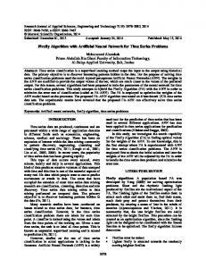
2.2 Explicit memory scheme As mentioned before, memory can improve the performance of optimisation algorithms in dynamic environments, especially for the cyclic ones. Figure 1, shows the block diagram of the explicit memory scheme used in this paper and its relationship with the proposed approach. It contains two memories: short-term memory and long-term memory.
History-driven firefly algorithm for optimisation in dynamic and uncertain environments Figure 1
329
Block diagram of explicit memory scheme and its relationship with the proposed approach Check similarity
Short-term memory
Long-term memory Insert item . . .
Hd-SFA algorithm
Insert node
Predict fitness
Figure 2
The structure of the each terminal and non-terminal node in short-term memory scheme Short-term memory xi [(L1i,U1i), (L2i,U2i), … (LDi, UDi)]
F(xi) [(L1i,U1i), (L2i,U2i), … (LDi, UDi)]
2.2.1 Short-term memory scheme The short-term memory is responsible for storing useful information about the individuals in the current environment, temporarily. After each environmental change, the useful information will transfer to the long-term memory in a summarised format. The aim of this memory is guiding the search direction to the promising areas by building a dynamic model of the problem over the time. This memory scheme uses the BSP tree for storing the valuable information during the run. In this tree, the whole search space is partitioned based on the distribution of the individuals in the environment. Each node in this tree represents a unique hyper-rectangular box in the search space and contains a representative solution for this sub-area. Suppose a parent node has two child nodes. The sub-areas represented by the child nodes are disjoint and their union is the sub-area of the parent. Figure 2 shows the structure of the short-term memory scheme used in this paper, in detail. The process of adding a new solution to the short-term memory is shown in Algorithm 1. After each fitness evaluation, first, the short-term memory – BSP tree – must be traversed to find the sub-area which the new solution belongs to (cur_node). Then, the new solution must be compared with the representative solution of that sub-area (xcur_node) to find a cut-off point. The middle of the largest difference between the all dimensions of these two solutions (x and xcur_node) will be selected as a cut-off point for creating two new children nodes. For more detail on the BSP tree construction as well as a numerical example, please refer to Chow and Yuen (2011).
Algorithm 1
ShortTermMem_insertNode()
Input: [x, f(x)] 1
begin
2
set cur_node to root node
3
while(cur_node has two child nodes: a and b)
4
Set Dimension j = arg max |a(k) – b(k)| where k ∈ [1, D]
5
if (|a(j) – x(j)| ≤ |b(j) – x(j)|) then
6
cur_node = a
7
else
8
cur_node = b
9
end if
10
end while
11
add two child nodes [xcur_node, F(xcur_node)] and [x, F(x)] to the parent node cur_node
12
convert the cur_node to a non-terminal node by removing [xcur_node, F(xcur_node)]
13
end
The proposed algorithm utilises this dynamic model (BSP tree) to approximate the fitness value of each individual exactly before actual fitness evaluation; this is done by Algorithm 2. Taking advantage of this dynamic model, the number of wasted fitness evaluations will decrease significantly and as a result the proposed algorithm is able to guide the search direction to the promising areas in the search space. As we can see in Algorithm 2, the preliminary steps are completely similar to the Algorithm 1. The only difference is from line 11 to 15. If the short-term memory is mature enough, the algorithm will return the fitness value of the
330
B. Nasiri and M.R. Meybodi
representative for the area which x belongs to, as a predicted value for solution x. The short-term memory is mature if the percentage of correct prediction is more than a pre-defined threshold value (maturity_threshold); this percentage can be calculated after each fitness evaluation.
LongTermMem_CheckSimilarity()
Input: [xtestPoint, f(xtestPoint)] 1 2
begin foreach env#i in long-term memory do
3
if |f(xtestPoint) – f(xtestPoint)env#i| < sim_thr then
4
f(xgOptima) = calculateFitness(xgOptimaenv#i)
Input: [x]
5
if |f(xgOptima) – f(xgOptima)env#i| < sim_thr then
begin
6
Algorithm 2
1
Algorithm 3
ShortTermMem_PredictIndividual()
return [true, env #i]
2
set cur_node to root node
7
3
while(cur_node has two child nodes: a and b)
8
4
Set Dimension j = arg max |a(k) – b(k)| where k ∈ [1, D]
9
end
10
return [false, –1];
if (|a(j) – x(j)| ≤ |b(j) – x(j)|) then
11
5 6
cur_node = a
7
cur_node = b
9
end if
10
end while
11
if the short-term memory is mature enough then return fcur_node as a predicted value for x
12
else
13
return ∞
14 15
end if end Output: [fcur_node]
Figure 3
The long-term memory scheme structure (see online version for colours)
Env#
Env#2
Test point
Env#3
Peak#1
Position
end Output: [flagSimilarity, SimilarEnv#]
else
8
end if end if
Peak#2
…
…
Fitness value
2.2.2 Long-term memory scheme The long-term memory is responsible for storing useful information about the previous environments in a summarised format. This useful information includes the positions and fitness values of the all discovered optima and also a pre-specified test solution in the past environments. The aim of this summarised memory is to provide the ability for the algorithm to remember the previous environments if re-occur in the future. The long-term memory is not destroyed by changes happening in the environment and it is permanent during the computation. However, it becomes more mature and more informative over the time. Figure 3 shows the structure of this summarised long-term memory scheme in detail.
In order to take advantage of this long-term memory, after each environmental change, the pre-specified test solution should be evaluated and the result must be compared with all the previous fitness values for this test solution in previous environments. If the difference was less than a predefined threshold then one can say maybe a previous environment is appeared again. To ensure this event, the algorithm will re-evaluate the global optima (xgOptima) for the most similar environment. By comparing the fitness values of the global optima in current environment and the most similar environment, we can ensure that a previous environment will appear again or not; this process is shown in Algorithm 3.
2.3 History-driven speciation-based firefly algorithm In this section, a novel swarm intelligence algorithm, namely HdSFA is presented for optimisation in dynamic environments. This algorithm store the landscape historical information in two distinct explicit memories and build a dynamic model of the problem over the time to improve the accuracy and convergence speed of the algorithm as more as possible. Also, taking advantage of these memories, the algorithm is able to remember the previous environment if re-occur in the future. HdSFA is a real-coded swarm intelligence algorithm. For a D-dimensional landscape S ⊂ RD, a solution x of HdSFA is a 1 by D real-valued vector, i.e., x ∈ RD. This algorithm employs two different populations – discoverer and tracker swarm – and also two different explicit memories to overcome the most challenges which exist in dynamic environments. Among them, we can mention to changes happening in the environment, transforming a local optima to a global, losing the position of all optima, losing diversity, converging two sub-species to one local optima, out-dated memory and short interval of time between two changes in the environment. The proposed algorithm begins with initialising the swarms and short-term and long-term memories. Afterwards, specie identification, change identification, discoverer and tracker swarm processing and also fine
History-driven firefly algorithm for optimisation in dynamic and uncertain environments tuning process are repeated until the number of fitness evaluations exceeds a pre-determined value. Algorithm 4 shows the block diagram of the HdSFA. In the following, each step in this algorithm is described in detail. Algorithm 4 1
Proposed algorithm – HdSFA
begin
2
call Initialisation()
3
repeat
4
call specie_identification()
5
call change_identification()
6
/*----discoverer swarm process begin------*/
7
if discoverer swarm is active then
8
call Swarm_Moving(Discoverer)
9
call Exclusion(Discoverer)
10
call Discoverer_Convergence_Checking()
331
discoverer swarm is configured somehow to explore the new promising areas in the search space effectively and efficiently. Once the discoverer swarm converged to a local optima, the k-best fireflies in it should be migrated to the tracker swarm, and the discoverer swarm should be re-initialised. The tracker swarm is responsible for chasing the discovered optima in the environment and does not have any firefly initially. Also, the short-term memory will initialise by adding the root node of the BSP tree. However, the long-term memory does not have any entry at first. Algorithm 6
Specie_identification()
input: [tracker swarm sw, rexcl] 1 2
begin Calculate distance matrix M where Mi,j is Euclidean distance between firefly i and j.
3
Calculate binary matrix B form M, where Bi,j is one if Mi,j is less than rexcl
11
end if
4
12
/*------ discoverer swarm process end------*/
5
Create a graph from matrix B and consider each connected graph as one specie.
6
Return the best firefly in each specie as a Gbest firefly
13
/*------ tracker swarm process begin------*/
14
foreach active swarm si in tracker S do
15
call Swarm_Moving(si)
16
end
17
call Specie_Freezing()
18
/*------ tracker swarm process end------*/
19
call fine_Tuning()
20 21
until stopping criterion is met end
Algorithm 5 1
Initialisation()
begin
7
end
8
Output: [list of Gbest firefly in each specie]
Algorithm 7 1
Change_identification()
begin
2
/* checking behavioural change in the algorithm*/
3
if the offline error increased more than k times sequentially then
4
/* ------ re-evaluate a test solution -------*/
5
f(xtest solution)new = calculate_fitness(xtest solution)
6
if f(xtest solution)new f(xtest solution)old then
2
Initialise the discoverer swarm Sdiscoverer = [xi]
7
/*------ change happened ------*/
3
for i=1, 2, …, Discoverer_number.
8
Add all discovered optima and pre-specified test solution into long-term memory.
end
9
Reinitialise short-term memory.
6
for i=1, 2, …, Tracker_number.
10
Re-evaluate the pre-specified test solution.
7
11
[flagSimilarity, SimilarEnv#] = LongTermMem_CheckSimilarity()
8
Initialise the short-term memory STM to consist of a root node only. end
12
if flagSimilarity is true then
9
Initialise the long-term memory LTM.
13
4 5
Initialise the tracker swarm Stracker = [xi]
10
Initialise the xtest-point and calculate f(xtest-point).
11
Activate the discoverer swarm.
12
foreach Firefly i in discoverer swarm F do
13
f(xi) = calculateFitness(xi)
14
ShortTermMem_insertNode([xi, f(xi)])
15 16
end end
The initialisation process is shown in Algorithm 5. It utilises two firefly swarms with different configurations and purposes for optimisation in dynamic environment. The
Restore position of all local optima from SimilarEnv# into current environment.
14
else Diversify all the fireflies in tracker swarm by adding a random value to the GBestPosition of each swarm between [-Vlength*P, Vlength*P]
15
16
end if
17 18 19
end if end if end
332
B. Nasiri and M.R. Meybodi
Specie identification is the first process in the main loop of the algorithm. The aim of this process is to identify the whole tracker swarms in the environment by doing a simple clustering as shown in Algorithm 7. Generally, there are two methods for discovering changes in dynamic environment, including re-evaluating a pre-specified test solution, and monitoring behavioural changes in the algorithm during the run. The current paper presents a hybrid approach based on two mentioned methods to discover any changes in the environment as shown in Algorithm 7. In this algorithm first, the trend of a performance KPI should be checked during k-latest fitness evaluations. This KPI is the mean of all fitness evaluations after the latest change in environment. If the trend of this KPI is increasing, the algorithm needs to re-evaluate the pre-specified test solution to ensure that any changes have happened in the environment. This hybrid approach can help the algorithm to decrease the number of wasted fitness evaluations for discovering changes in the environment. In this paper, we used 4 for the k value. After the change is discovered in the environment, two actions should be done. First, all discovered optima should be added to the long-term memory and then the fireflies in each tracker species should be diversified. This diversification can be done by adding a random value in range of [–Vlength*P, Vlength*P] to the Gbest Position of each firefly specie. Algorithm 8
Swarm_Moving()
2
begin
The fitness value of the each firefly should be predicted by the BSP tree whenever the firefly moves to another position. If the predicted value for this new position is equal or better than its Pbest fitness value, the actual fitness evaluation will be happened on new position of the firefly.
3
The position of each firefly will change if the fitness value of the new position is better than the current position.
Algorithm 9 1
Move firefly i towards j based Equation (1)
6
end if
7
p(xinew)=ShortTermMem_PredictIndividual(xinew)
8
if p(xi
new
old
)