errors. Neural networks and stochastic models have been widely used in document analysis .... ori probability is calculated but in the same time the Viterbi.
HMM based Viterbi paths for rejection correction in a convolutional neural network classifier Hubert Cecotti, Szilard Vajda and Abdel Bela¨ıd READ Group LORIA/CNRS Campus Scientifique BP 239 54506 Vandoeuvre-les-Nancy cedex France cecotti,vajda,abelaid�@loria.fr Abstract This paper presents a rejection strategy for a convolutional neural network. The method is based on Viterbi paths generated by a context based 2D stochastic model for rejected image correction. The rejection strategy is an important issue in neural network theory. The challenge is to find rules, which determine if an image is correctly classified or not. Applying strong rules leads to the rejection of many well-recognized patterns whereas weak rules do not always involve a strong decrease of erroneous patterns. We propose to use in several ways the knowledge of an external stochastic model so called NSHP-HMM (Non Symmetric Half-Plane Hidden Markov Model) for re-evaluating the rejected patterns.
1 Introduction The rejection estimation is an important problem in order to obtain a reliable system [2, 3, 4, 9]. Considering a classifier, the optimal rejection would be to only reject errors. Neural networks and stochastic models have been widely used in document analysis system [5]. Neural networks have proved to be very effective in character recognition, and stochastic models have been applied with success in word recognition for recognition and normalization. As neural networks have a fixed input, deformed images may not be well recognized. A solution can be to correct rejected patterns thanks to an external system. Stochastic models like the NSHP-HMM based on Markov random fields, which works on pixel level, evaluate images by estimating probabilities on observations. The strategy described uses the neural network as the main classifier and the stochastic classifier as a way to improve the reliability of the systems. This relationship is possible thanks to knowledge extracted from the Viterbi paths from the NSHP-HMM. In the first section, we describe the different parts of the system: the
convolutional neural network, the rejection criterion and the NSHP-HMM model. The second section will show how can an NSHP-HMM be used to normalize an input image and change the network topology. The last section is dedicated to the experiments and describes the rejection improvement achieved by an external stochastic model.
2 System overview We propose to combine two systems: a neural networks based on convolutional layers and a HMM based model: NSHP-HMM. The first system is dedicated to classification; the second one is only used for normalization purpose. Both models are first trained separately. During the test phase, the neural network first processes images. If an image is rejected, it is corrected thanks to the Viterbi paths generated by the HMM, which give us a different vision of the image. If this new image created by the average HMM models answers to rejection criteria then it is accepted, otherwise it stays rejected. Considering the sense how a pattern can be read, several NSHP-HMM models can be built. The image is normalized with a combination of a vertical and horizontal NSHP-HMM model then it is given as input to the neural network. We finally use a voting scheme to find the correct class between all the corrected images that were not rejected. The rejection is based on 2 criteria: The mean recognition rate of each class on the learning database. The mean distance between the first and the second best class on the learning database. If an image does not correspond to one of these rules then the pattern is considered as being rejected. The purpose of the method proposed is to use Viterbi paths extracted from the NSHP-HMM model and to show how it can improve the relevance of the recognition.
2.1 Convolutional neural network The goal of the topology based on convolutional neural network is to classify the image given as input by analyzing it through different learnt “filters”. Each convolutional layer is composed of several maps, each map corresponds to a transformation of the image. These transformations extract features like edges, lines, etc [5, 8]. The proposed neural network is composed of 5 layers: The first one corresponds to the input image. The image is normalized by its center and reduced to a size of 29*29. The next two layers correspond to the information extraction, performed by convolutions. They are described as follows: – The second layer is composed of 10 maps; each one corresponds to a specific image transformation by convolution and sub-sampling reducing its size. For each map, all the neurons have the same input link number and share their weights.
As in our model the � was chosen as being a � �� order neighborhood, the NSHP-HMM is sub-divided in 4 NSHPHMM. Such a division of the model is necessary due the non-symmetric sampling of the image pattern. Each NSHPHMM can be considered a separate classifier representing the different reading senses (right to left, left to right, bottom to top and top to bottom) of the model. In the original model the a posteriori probabilities given by the different sub-models are integrated. During the Viterbi algorithm, which is basically a dynamic programming, an a posteriori probability is calculated but in the same time the Viterbi path is also conserved. The meaning of this path is to track which state reads which observation [6]. Vertical and horizontal NSHP-HMM have been considered as shown in figure 1. The first row represents vertical models with different reading sense to extract horizontal elasticity knowledge whereas the second row represents horizontal models for extracting vertical elasticity knowledge. Indeed, all these models are initially the same but as they are trained on images in different orientations and senses, they produce models with different meanings.
– The third layer is composed of 50 maps, each map representing a convolution of the combination of 5 maps coming from the previous layer. In each map, the link weights are shared by all its neurons. A pivot neuron is considered in each map. Its links synthesize the receptive field. In this case an input link is described by a special link to the weight value. The last two layers are fully connected. The last one corresponds to the output: 10 neurons.
Figure 1. NSHP-HMM models.
2.2 NSHP-HMM model A stochastic model, so called NSHP-HMM (Non Symmetric Half-Plane Hidden Markov Model), originally designed for handwritten word recognition has been used for this purpose. The model also achieved the same success in handwritten digit recognition [7]. The originality of this method resides in coupling a context based local vision performed by a NSHP with a HMM giving horizontal elasticity to the model. It operates on pixel level, analyzing pixel columns, which are viewed as the random field realizations considering a given � neighborhood. Let be the image having � rows and � columns observed by the NSHP. The joint field mass probability � � � of the image can be computed following the chain decomposition rule of conditional probabilities: �
�
� �� �
�
� �
�
� �
�
� �� � �
3 Viterbi paths for correction The Viterbi paths are used to normalize the image given as input to the neural network. Let an image � ��� � � of size � and 80 NSHP-HMM models. For each of the 10 classes, there exist 8 different models. The 4 first models are vertical models, allowing a synthesis of the columns for each reading direction. The same way, the 4 last models are horizontal and they allow a synthesis of rows. Combining the vertical and horizontal models, the image can be transformed in 16 (4*4) new images. The figure 2 presents the fusion of horizontal and vertical model in order to obtain a new image normalized in 2 dimensions. Each NSHP-HMM model is defined by � states in the main HMM, and observations. The use of the NSHP-HMM, and particularly its associated Viterbi paths, consists in transforming the input image in function of the different class models. Two
solutions can be considered for using the Viterbi paths for image normalization. In the first case, the output image has the size � �� � � ��. The new images have the same size as the number of states in the NSHP-HMM. This new image is like a sub-sampling of the original input image. This method has been used for image normalization by averaging the columns read by the same state of the NSHP-HMM. The classifiers used were SVM (Support Vector Machines) and neural networks [1]. In the second solution the output image has the same size of the input image: � . In both cases the transformation is applied in two steps. The first one uses a vertical NSHP-HMM where each main state observes one or several columns. The output image size at this step is � � ��. The second step uses a horizontal NSHP-HMM where each main state observes one or several rows. The normalization purpose is to redistribute fairly the observations between states in order to obtain a synthetic image. In the ideal case of a reduction with deformations, each state should observe only 2 columns. Let � � and �� the values corresponding to the 2 new observations of the �� state, with � � �. For each row of the image, we find the points sequences observed by a same state. For each sequence, the new observations values are calculated. These observations correspond to what the NSHP-HMM should see if the image would be well balanced. The new observations values are defined by: In the first solution: ��
�
� �� � ��
�
�
�
�
�
� �� � � �
� ��
In the second solution: ��
�
�
�
� �
��
�
�� �
��
�
�
�
�
�
� �
� �
� �
��
�
�
�
� � � � � � ��� � � � � � � �
� � � �� � � �
� ��
Where � represents the number of points observed by the �� state, � � � and � ��� �� represents the gray density of a point of coordinate ��� � �. This process is iterated again using a horizontal NSHP-HMM model for normalizing the rows. In this case, rows and columns are exchanged of � ��� � � for computing � � and �� . The first solution assigns to each state the mean value of each observed point. That corresponds to a sub-sampling of the image. Using the second solution, the image is not reduced. The observations balance in the image is just restored function to what it should be better to observe. With this method, the variation between points observed by a same state keeps its meaning. Whereas the mean erases the
difference between points and can delete some information like contrast variation, this difference is always conserved by 2 observations. For example, let a sequence (1,3,4) observed by a state. In the first case, these observations are synthesized by the mean of their values: �� � � � � �. In a sub-sampling, the 2 ideal observations for homogeneous observations in the image would be also
�. In the second case, the first new observation is defined by �� � ��� � ��� � � � � � � whereas the second one has the value �� � � � � � � � � �� � � �� �. This method allows keeping details of the image without reducing the size of the image to the state number of the NSHP-HMM. In the case of a heterogeneous sequence like (0,0,9), it’s much better to observe the sequence (0,6) than the sequence (3,3).
Figure 2. NSHP-HMM models fusion.
4 Experiments The system has been tested on the MNIST database. This well-known benchmark database contains separated handwritten digit images of � � � in gray level. The learning set contains 60000 images (50000 used for real learning and 10000 used to choose when to stop the learning). The test set contains 10000 images. The table 1 presents the recognition rate with (B) and without (A) rejection criteria. The tables 2 and 3 show the results obtained by normalizing rejected images by using the Viterbi paths from the different NSHP-HMM models. The figure 3 shows the global recognition system using 16 normalization hypothesis. The first and second table corresponds to the first and second solution respectively described in 3. In the two tables, the first column represents the number of patterns not rejected, recognized as a same class, needed to accept the image. For a low number of new images accepted the error rates is still high (bad correction) whereas after about 8 accepted patterns the correction is effective. The results obtained illustrate the improvement of the number of recognized patterns while keeping a very low error rate. Both solutions described in 3 give about the same results. Even with a separate learning, the NSHM-HMM model succeeds to supplement the neural network by using its synthesis class models.
Figure 3. Global System.
Method A B
Table 1. MNIST results. Recognition Rejection 98.73 0.00 88.98 10.95
Error 1.27 0.07
Table 2. Recognition rate function to the minimal number of corrected patterns accepted. Accepted pattern Recognition Rejection Error 1 94.52 2.63 2.85 2 93.13 5.20 1.67 3 92.04 7.06 0.90 4 91.25 8.15 0.60 5 90.17 9.51 0.32 6 89.88 9.90 0.22 7 89.65 10.18 0.17 8 89.54 10.34 0.12 9 89.40 10.50 0.10 10 89.29 10.63 0.08 11 89.23 10.70 0.07 12 89.16 10.77 0.07 13 89.10 10.83 0.07 14 89.06 10.87 0.07 15 89.02 10.91 0.07 16 88.98 10.95 0.07
Table 3. Recognition rate function to the minimal number of corrected patterns accepted. Accepted pattern Recognition Rejection Error 1 94.69 2.16 3.15 2 93.50 4.60 1.90 3 92.40 6.55 1.05 4 91.66 7.70 0.64 5 91.01 8.63 0.36 6 90.50 9.20 0.30 7 90.14 9.64 0.22 8 89.80 10.03 0.17 9 89.57 10.31 0.12 10 89.44 10.45 0.11 11 89.36 10.54 0.10 12 89.24 10.66 0.10 13 89.16 10.76 0.08 14 89.08 10.85 0.07 15 89.02 10.91 0.07 16 89.00 10.93 0.07
there was no relationship during the learning between the neural network and the NSHP-HMM, the NSHP-HMM allowed by its synthetic model to correct patterns. It improves the number of recognized patterns while keeping a very low error rate.
5 Conclusion
References
The rejection processing is a difficult task to optimize in order to reject only erroneous patterns. A method using an external stochastic model has been used for correcting the rejected patterns. The Viterbi paths are extracted from several NSHP-HMM models. These paths allow a vertical and horizontal normalization of the image. We have proposed two methods for using these paths. These two methods allow to correct some patterns previously rejected. Although
[1] C. Choisy and A. Belaid. Handwriting recognition using local methods for normalization and global methods for recognition. In In Proc. of 6th International Conference on Document Analysis and Recognition, pp. 23-27, 2001. [2] C. Chow. On optimum recognition error and reject tradeoff. In IEEE. Trans. Information Theory, vol 16, pp. 41-46, 1970. [3] N. Gorksi. Optimizing error-reject trade off in recognition systems. In 4th International Conference Document Analysis and Recogntion, pp. 556-559, Ulm, Germany, 1997.
[4] L. Koerich. Rejection strategies for handwritten word recognition. In to appear in 9th International Workshop on Frontiers in Handwriting Recognition (IWFHR-9), 2004. [5] Y. LeCun, L. Bottou, Y. Bengio, and P. Haffner. Gradientbased learning applied to document recognition. In Proceedings of the IEEE, vol. 86, n11, pp. 2278-2324., 1998. [6] L. Rabiner. A tutorial on hidden markov models and selected applications in speech recognition. In Proceedings of IEEE, volume 77, pp. 257-285, 1989. [7] G. Saon and A. Belaid. High performance unconstrained word recognition system combining hmms and markov random fields. In IJPRAI, vol. 11, no. 5, 1997, pp. 771-788, 1997. [8] L. Teow and K.-F. Loe. Robust vision-based features and classification schemes for off-line handwritten digit recognition. In Pattern Recognition 35 (11): pp. 2355-2364, 2002. [9] M. Zimmermann, R. Bertolami, and H. Bunke. Rejection strategies for offline handwritten sentence recognition. In 17th International Conference on Pattern Recognition (ICPR) Volume II, pp. 550-553, Cambridge, United Kingdom, 2004.