Holistic Processing Develops Because it is Good - UCSD CSE

Holistic Processing Develops Because it is Good Lingyun Zhang and Garrison W. Cottrell {lingyun,gary}@cs.ucsd.edu UCSD Computer Science and Engineering 9500 Gilman Dr., La Jolla, CA 92093-0114 USA

Abstract In this paper, we investigate the question, “what are the best features for face identification?” Ullman et al. used mutual information as measurement of how good a feature is for a class [Ullman et al., 2002]. Their experiments suggested that features of intermediate complexity are best in tasks of face vs. non-face and cars vs. non-cars. We are interested in the tasks of face identification and expression classification. We applied Ullman’s technique of finding features with high mutual information with category labels to the tasks. We found that features of large sizes convey the most information about face identity. Local features such as eyes and mouth are informative for identity in the context of large face areas. Yet they are not very informative by themselves, especially for an image set with high variability of facial expressions. On the other hand, small sized features around the eyes and mouth contain relatively high information for expression classification. This suggests that the appropriate feature sizes are task dependent. We suggest that holistic processing of faces has developed because these features are optimal for face identification.

Introduction In this paper, we investigated what the best features are for face identification. Face identification is a subordinate level task [Diamond and Carey, 1986] and is known to be holistic or configural. Holistic processing is typically taken to mean that the context of the whole face has an important contribution to processing the parts, and suggests that subjects use some kind of whole-face representation when processing faces: they have difficulty recognizing parts of the face in isolation, and they have difficulty ignoring parts of the face when making judgments about another part [Carey and Diamond, 1977, Carey and Diamond, 1994, Farah et al., 1995, Tanaka and Farah, 1993]. Configural processing means that subjects are sensitive to the relationships between the parts, e.g., the spacing between the eyes. Ullman et al. proposed using a measure of the mutual information between features and categories to find the features that provide the most information relevant to classification problems [Ullman et al., 2002]. Their experiments showed that features of intermediate complexity in size and resolution were best for classification (faces vs. non-faces, cars vs. non-cars). Figure 1 shows the combination of features they found for faces and cars. The intuition is that small, simple features are likely

to be found in both targets and non-targets (high false alarms) and large, specific features are unlikely to generalize to more than the image they are found in (high misses). Intermediate complexity gives a good balance between the trade-offs of misses and false alarms. They suggested that these features are represented after the encoding of simple features in V1 but before the encoding of complex object views in anterior IT cortex, and that the features of intermediate complexity are the natural result of being selected for visual classification.

Figure 1: The set of fragments extracted by maximizing the amount of information delivered. (a) The features found for faces. (b) Examples of images in the training set. (c) The features found for cars. (adapted from [Ullman et al., 2002] with author’s permission).

Will features that are good for telling faces from objects be good for identification? We expect more specific features would be needed for face identification. Our results show that features of large size are best for face identity classification. Local features are not as informative as global ones because the variances of local features such as eyes and mouth across different images of the same person due to expressions and other factors are comparable to those across individuals. We also show that the features optimal for expression classification are of small sizes. The result suggests that holistic processing for faces has been developed simply because it is good or even necessary for accurate identification.

Methods Data Set 36 frontal images of 6 individuals (6 images each) from the FERET database were used [Phillips et al., 1998]. The images were aligned by rotating, scaling and cropping [Zhang and Cottrell, 2004]. Figure 2 shows the normalized face images, where each row is an individual.

Figure 3: A Gabor function is constructed by multiplying a Gaussian function by sinusoidal function [Daugman, 1985]. We used five scales with eight orientations.

(Figure 4). Gabor filter responses of a certain frequency with all orientations on these grid points are collected. Hence, one “patch” is a concatenated vector of 8 Gabor filter responses at each grid point. Patches were of different locations, sizes and frequencies. We collect patches of size (2n − 1) ∗ (2m − 1) of all possible locations and frequencies, i.e. size 1 ∗ 1, 1 ∗ 3, 1 ∗ 5, ..., 3 ∗ 1, 3 ∗ 3, ... at all possible locations and frequencies.

Figure 4: Patches of different centers, sizes and Gabor filter frequencies were taken from the images.

Figure 2: The 6 individual by 6 images from FERET. Each row is an individual.

Preprocessing Ullman et al. used raw pixel patterns of varying size and resolution in their study, which is an unrealistic cortical representation of an image. Research suggests that the receptive fields of the striate neurons are restricted to small regions of space, responding to narrow ranges of stimulus orientation and spatial frequency [Jones and Palmer, 1987]. DeValois et al. [DeValois and DeValois, 1988] mapped the receptive fields of V1 cells and found evidence for multiple loci of excitation and inhibition. Two-D Gabor filters [Daugman, 1985](Figure 3) have been found to fit the 2D spatial response profile of simple cells quite well [Jones and Palmer, 1987]. The complex cells are found to approximately compute the magnitudes of the responses [Pollen and Ronner, 1983]. In the preprocessing, the images were filtered with a set of overlapping 2-D Gabor filters in quadrature pairs at five scales and eight orientations. Gabor filter responses are sampled at every grid point on a rigid 23 by 15 grid (Figure 4). [Dailey et al., 2002]. The magnitudes of the filter responses were then z-scored across images (subtract mean and divide by standard deviation so as to be zero mean and one standard deviation, so that every response is treated equally).

Patches Patches of Gabor filter responses were taken from the images. A patch is a rectangle sample of grid points

Because we have normalized our images, we can define corresponding patches in image coordinates. We define corresponding patches to be the patches of the same position, size and Gabor filter frequency across images. (Figure 5). A patch is said to be present in an image if the corresponding patch in the images has a correlation bigger than the threshold (a parameter) with the patch. Here we did not search across location for patch matches because the images were all normalized to approximately the same layout.

Figure 5: Corresponding patches across images.

Measurements by Mutual Information Following Ullman et al.([Ullman et al., 2002]), the usefulness of the patches for face identification was measured by mutual information: I(C; F ) = H(C) − H(C|F )

(1)

In the equation, H denotes entropy which measures the uncertainty of the variable. Thus I(C; F ) measures how much the uncertainty of variable C is reduced by knowing variable F . In other words, it measures how much information F conveys about C. In our implementation, C and F are both binary variables. C denotes the binary variable of “the image is the

face of the individual or not” for a certain individual. F denotes the binary variable of “presence of the patch in the image or not” for a certain patch. For patch i in image j, C = 1 for the 6 images belonging to the same individual of image j, C = 0 for the rest 30 images; F = 1 for images in which patch i is present, F = 0 otherwise. The mutual information can thus be calculated as follows: ¯ log p(C) ¯ I(C; F ) = −p(C) log p(C) − p(C) ¯ ¯ +p(F )(p(C|F ) log p(C|F ) + p(C|F ) log p(C|F )) ¯ F¯ ) log p(C| ¯ F¯ )) +p(F¯ )(p(C|F¯ ) log p(C|F¯ ) + p(C| Mutual information is calculated between every individual and the patches from the images of the individual. This measures how much the presence of the patch predicts identity. The best threshold for “presence of a patch” was found for each patch by brute force search, from −0.9 to 0.9 by steps of 0.1. The threshold with the highest mutual information was used for that patch. This is after the fashion of Ullman et al. Averages across corresponding patches from images belonging to the same individual were taken to measure how much a patch predicts this individual. Averages across individuals were taken to measure how much this patch predicts identity.

Face Identification The results showed that patches of large sizes had the most information about identity. The best patches are not whole face patches, but they do encode at least two “traditional” features (eyes, nose, mouth). That is, they encode the eye in the context of the nose and vice versa. Figure 6 shows several patches with highest mutual information. Figure 7 displays the mutual information of all patches centered on the image. Large patches are usually preferred given same frequency scale and position.

Figure 6: The best 6 patches. Frequency of 1 to 5 denotes from the highest Gabor filter frequency to the lowest. These are the patches with the highest mutual information. Note that some are similar to others because we do not eliminate redundancy in the results reported in this paper, i.e., the best combination was not considered at this stage as in Ullman et al.’s work.

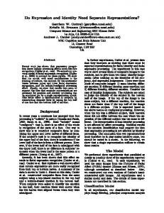
Figure 7: The mutual information of all the patches centered at the image center. The x axis is the width of the patch, and the y axis is the height of the patch. The big patches are on the top right while small patches are on the bottom left. The good patches are of large sizes.

Winner Take All In this experiment, the classification was carried out by voting of the patches. The best 100 (this number was arbitrarily used in the experiments reported in this paper) patches and their thresholds were calculated from the training set. For the test set, 1 image of each individual was taken as a “known” image. The other 30 were “novel.” For each novel image, the identity was decided by calculating how many of the best 100 patches from a “known” image were present in this image and taking the identity of the image to be the identity of the individual with the most patches present. The 36 images of the test set were divided to 6 sets of “known” images (the columns of Figure 8), and with each as the “known” image set, the error rate was calculated. Table 1 shows the results. One issue that arises is how the Gabor filter responses on the test set are normalized by z-scoring. We consider the z-score to be an adaptation on an individual neuron level, that is, each complex cell is adjusting its response to be 0-mean and unit standard deviation. If this is slow, then the training set z-scoring should be used. But if this is fast (the subject adapts to the test set), then the test set should be used. We report both for completeness. That the test set is z-scored by the test set means that the test set’s mean and standard deviation are used, while that the test set is z-scored by the training set means that the training set’s are used. Note that there is a decrease in performance when the test set is z-scored by the training set’s mean and standard deviation. Table Training set FERET1 FERET1 FERET2 FERET2

1: Error rate in “winner takes all” Test Test set Error rate set z-scored by (out of 180) FERET2 Test set 3.3% (6) FERET2 Training set 8.3% (15) FERET1 Test set 6.1%(11) FERET1 Training set 11.1%(20)

Generalization To find out how well the patches we found generalize to other face images, we extracted another set of 36 images (6 individual by 6 images each) from FERET (Figure 8). In the following text, the earlier set will be referred as “FERET1” and this new set as “FERET2”. We tested generalization in 2 ways.

Thresholding In this experiment, we set a threshold for “accepting the identity”, if the count of the patches (from a “known image”) presented (in a novel one) is above the threshold, then accept the identity of the known image as the novel image’s identity. In this formulation, none or more than one identity can be accepted

Figure 9: F-measure of FERET1. Table 2: Threshold = 29, Training set = FERET1, Test set = FERET2 Test set Miss False alarm z-scored by (out of 180) (out of 900) Test set 2.2% (4) 2.2% (20) Training set 1.1%(2) 49.6% (446)

for the training set is maximized (0.993) when threshold is in range [34,42]. The results are calculated by using threshold of 38 (the midpoint of [34,42]) in the test set. Figure 8: The new set 6 individual by 6 images from FERET. Each row is an individual.

for one image. Note the threshold is the number of the present patches and is different from the threshold for deciding whether a patch is present or not. For the training set, the 100 best patches were again calculated. Then the evaluation matrix of true positive, false positive etc. is calculated by thresholding the number of presented patches. The Fmeasure[Salton and McGill, 1983] can thus be calculated: F − measure =

2 ∗ recall ∗ precision recall + precision

(2)

where recall = precision =

true positive true positive + f alse negative

(3)

true positive true positive + f alse positive

(4)

Figure 9 plots how the F-measure of FERET1 changes with the threshold. The F-measure is maximized (0.990) when the threshold is from range [28,30]. We then applied the threshold of 29 (the midpoint of [28,30]) to the test set of FERET. Table 2 shows the results. The first row shows the results when the test set is z-scored with its own mean and standard deviation and the second row with the training set’s. Table 3 shows the results when using FERET2 as training set and FERET1 as test set. The F-measure

Table 3: Threshold = 38, Training set = FERET2, Test set = FERET1 Test set Miss False alarm z-scored by (out of 180) (out of 900) Test set 11.1% (20) 1.3% (12) Training set 3.3%(6) 24.2% (218) The results generally got worse when z-scored with the training set’s mean and standard deviation. The effect is larger in the thresholding method than the voting one. This may because the training set’s mean is off-center from the test set to some degree. The patches are thus distorted and more correlated. In the voting method, the number of the present patches for the correct identity goes up with the wrong ones so the maxima are not affected too much(Table 1), while in the threshold method, misses decreased but many more false alarms occurred (Table 2,3) because the counts goes up. We would expect a larger training set should help because the center (the mean) would be more general. The results were far from perfect. Yet it was encouraging because in the tests, classification (or identity acceptance/rejection) was based on only one image per person, and generalized to five.

Expression Classification The results from last section showed that local features such as eyes and mouth are informative for identity in the context of large face areas but not by themselves.

Why are the main features on the face such as the eyes and the mouth not good enough? Why features need to include configural information? Our hypothesis is that local features vary a lot in different images of the same individual due to expression and other possible factors. This variability could be comparable to that across different individuals, which makes local features bad predictors for identities. For example, “happy eyes” from different individuals could be more similar to each other than “sad eyes” and “happy eyes” from one individual. Thus, depending on the similarities of local features, a happy face would be more likely to be matched to another happy face rather than those of the same identity. Following this reasoning, we would expect local features to be good predictors of expressions. To test our hypothesis, we did similar experiments on 36 images from POFA [Ekman and Friesen, 1976] (6 individual by 6 expressions, Figure 10). Figure 11 shows the best patch found for each expression. (We do not show the best ones for identification here for comparison because the hairlines are always being chosen. This is due to the fact that hairstyle of each individual dose not change in POFA, so it is the most reliable identification feature.)

Figure 11: The best patches for each expression. The numbers in the parentheses are the Gabor filter frequencies, 1 the highest and 5 the lowest. Note that because the frequency for the sad one is of low frequency, which means the patch covers more spatial extent than would be suggested by the patch size.

we examined how smaller patches are doing for identities. Figure 12 shows mutual information between 3 by 3 grid sized patches and identity of the POFA set. Note that patches centered on the eyes or mouth are very bad for classifying identities although they can be good indicator of expressions. Patches around hairlines are better because the individuals’ hairstyles do not change in this image set. Figure 13 shows that of the image set from FERET1. In this image set, the expressions of individuals do not change as dramatically as those in the POFA, so the patches around local features such as mouth and eyes do not show a drop in mutual information, but they are not as informative as the large ones we showed earlier (Figure 7).

Figure 12: The mutual information of all 3*3 grid size patches for identity with the 36 images from POFA. The patches centered on the eyes and the nose are bad indicators of identity because the variability within an individual is largely due to different expressions.

Figure 13: The mutual information of all 3*3 grid size patches for identity with the 36 images from FERET.

Discussion Figure 10: The 6 individual by 6 expression face images from POFA. Each row is an individual. Each column is an expression.

As expected, local features are good predictors for expressions, which make them unlikely to be good predictors for identities at the same time. To take a closer look,

We applied Ullman et al.’s technique of finding features with high mutual information with category labels to the tasks of face identification and expression classification. Our results showed that large areas of faces are informative for the identity, or rather, individual features need to be processed in context of larger areas of the face to be informative. On the other hand, local features are informative for expression classification. This result may suggest why holistic processing of faces has developed -

simply because it is good or even necessary for identification, given individual features are not very useful by themselves.

[Phillips et al., 1998] Phillips, J., Wechsler, H., Huang, J., and Rauss, P. J. (1998). The feret database and evaluation procedure for face-recognition algorithms. Image and Vision Computing, 16(5):295–306.

Future Work

[Pollen and Ronner, 1983] Pollen, D. A. and Ronner, S. (1983). Visual cortical neurons as localized spatial frequency filters. ieee transactions on systems. IEEE Transactions on Systems, Man, and Cybernetics, 13(5):907–916.

A virtue of what we have done is its simplicity, but we also want to explore other issues. First, we do not search across images for patch matches, i.e. we assume a location as well. We would like to further investigate matching patches at multiple locations. Then the training can possibly be done without aligning the images. Second, in the current work, mutual information of patches is calculated separately. We would like to further looking into what combinations of features are optimal. Third, as Ullman et al. did, weights can be associated to patches depending how much information they provide for the classification task. Last but not least, the generalization tests we did are limited. We would like to further test our method and hypothesis with larger and more varied data sets.

Acknowledgement We thank PEN (Perceptual Expertise Network) for valuable discussions, GURU (Gary’s Unbelievable Research Unit) for suggestions. This research project was supported by NIMH grant MH57075 to GWC.

References [Carey and Diamond, 1977] Carey, S. and Diamond, R. (1977). From piecemeal to configurational representation of faces. Science, 195:213–313. [Carey and Diamond, 1994] Carey, S. and Diamond, R. (1994). Are faces perceived as configuration more by adults than by children? Visual Cognition, 1:253–274. [Dailey et al., 2002] Dailey, M. N., Cottrell, G. W., Padgett, C., and Adolphs, R. (2002). Empath: A neural network that categorizes facial expressions. Journal of Cognitive Neuroscience, 14(8):1158–1173. [Daugman, 1985] Daugman, J. G. (1985). Uncertainty relation for resolution in space, spacial frequency, and orientation optimized by two-dimensional visual cortical filters. Journal of the Optical Society of American A, 2:1160–1169. [DeValois and DeValois, 1988] DeValois, R. L. and DeValois, K. K. (1988). Spatial Vision. Oxford University Press. [Diamond and Carey, 1986] Diamond, R. and Carey, S. (1986). Why faces are and are not special: an effect of expertise. Journal of Experimantal Psychology: General, 115(2):107–117. [Ekman and Friesen, 1976] Ekman, P. and Friesen, W. (1976). Pictures of Facial Affect. Consulting Psychologists Press. [Farah et al., 1995] Farah, M., Levinson, K., and Klein, K. (1995). Face perception and within-category discrimination in prosopagnosia. Neuropsychologia, 33:661–674. [Jones and Palmer, 1987] Jones, J. P. and Palmer, L. A. (1987). An evaluation of the two-dimensional gabor filter model of simple receptive fields in cat striate cortex. Journal of Neurophysiology, 58(6):1233–1258.

[Salton and McGill, 1983] Salton, G. and McGill, M. (1983). Introduction to Modern Information Retrieval. McGrawHill. [Tanaka and Farah, 1993] Tanaka, J. and Farah, M. (1993). Parts and wholes in face recognition. The Quarterly Journal of Experimental Psychology: Human Experimental Psychology, 46A(2):225–245. [Ullman et al., 2002] Ullman, S., Vidal-Naquet, M., and Sali, E. (2002). Visual features of intermediate complexity and their use in classification. Nature Neuroscience, 5(7):682– 687. [Zhang and Cottrell, 2004] Zhang, L. and Cottrell, G. W. (2004). When holistic processing is not enough: Local features save the day. In Proceedings of the 26th Annual Cognitive Science Conference, Chicago, Illinois. Cognitive Science Society.