arXiv:hep-th/0008004v3 12 Oct 2001 · hep-th/0008004. Phys. Lett. B 519 (2001) 111-120 [Secs II-IV only]. Holography and field-to-particle transition in sigma ...
hep-th/0008004 Phys. Lett. B 519 (2001) 111-120 [Secs II-IV only]
Holography and field-to-particle transition in sigma model, dilaton and supergravity: Point particle as end product of field theory and seed of string-brane approach Konstantin G. Zloshchastiev
arXiv:hep-th/0008004v3 12 Oct 2001
Department of Physics, National University of Singapore, Singapore 119260, Republic of Singapore and Department of Theoretical Physics, Dnepropetrovsk State University, Dnepropetrovsk 49050, Ukraine ( Received: 1 Aug 2000 [LANL], 19 Jul 2001 [PLB] ) The paper consists of the two parts that are devoted to separate problems and hence seem to be independent of each other but for a first look only. In the Part one the field-to-particle transition formalism is applied to the sigma model (field counterpart of string theory), dilaton gravity and gauged supergravity 0-brane solutions. In addition to the fact that the field-to-particle transition is of interest itself it can be regarded also as the nontrivial dynamical dimensional reduction which takes into account field fluctuations as well as one can treat it as the method of the consistent quantization in the vicinity of the nontrivial vacuum induced by a field solution. It is explicitly shown that in all the cases the end product of the approach is the so-called non-minimal point particle. In view of this it is conjectured that this is not a mere coincidence, and point particles are not only the end product of the field theory but also the underlying base of material world’s hierarchy: if high-dimensional point particles are the base then the strings can be regarded as their path trajectories, etc. The Part two is devoted to the formal axiomatics of the string-brane approach - there we deepen the abovementioned conjecture and make it more accurate. It is shown that a point particle can be regarded as an extended object from the viewpoint of a macroscopic measurement - it is actually observed as the “cloud” consisting of the particle’s virtual paths, therefore, for an observer the real particle cannot be seen as a point object anymore. However, it cannot be supposed also as a continuous extended object unless we average over all the deviations. Once we have performed the averaging we obtain the extended object, metabrane, which can be considered “as is”, i.e., regardless of the underlying microstructure because it possesses the new set of the (collective) degrees of freedom. This brane may appear to be the composite string-brane object consisting of the microscopical objects (strings) and cosmological-size ones (3-brane) where the size of a corresponding embedding is governed by the weight constants arising along with the decomposition. Finally, we outline the picture which unifies both parts and sets the role of each of them. PACS number(s): 04.60.Kz, 04.65.+e, 11.25.Sq, 11.27.+d, 12.60.Jv
ories but, nevertheless, the problem of the origin of matter remains to be still open and important, especially in what concerns the theoretical explanation of the fundamental properties of observable particles. The most intuitive idea here is to regard the localized field solutions as the corpuscles of matter. However, if one tries to fit such a field solution in the particle interpretation one eventually encounters the problem of how to treat the field fluctuations in terms of particle degrees of freedom. In fact, it is caused by the fact that a field solution is still a field and hence it has an infinite number of degrees of freedom whereas a particle has a finite number of them. Therefore, it is necessary to correctly handle this circumstance to be protected from deep contradictions. Thus, in Sec. II A we demonstrate the field-to-particle transition for the N -component 2D sigma model or, equivalently, simple bosonic string in the N -dimensional spacetime (the latter is supposed flat for simplicity but the external potential U is included and can be treated as effective). Minimizing the action with respect to field fluctuations around a chosen solution, we remove zero modes and eventually obtain the effective
I. INTRODUCTION
In the part one of present paper we try to achieve the three main aims: (i) construction of the consistent classical and quantum field-to-particle transition formalism for the N -component 2D sigma model, (ii) application of this approach to classical and quantum dilaton gravity, (iii) application to supergravity 0-brane solutions and connection with the holographic principle. Let us consider them in more details. Field-to-particle transition. The study of the field-toparticle transition formalism itself lies within the wellknown dream program of constructing a theory which would not contain matter as external postulated entity but would consider fields as sources of matter and particles as special field configurations. Such a program was inspired probably first by Lorentz and Poincar´e and since that time many efforts have been made to come it into reality, one may recall the Einstein’s, Klein’s and Heisenberg’s attempts. The discovery of fermionic fields and success of Standard Model decreased interest to such the-
1
plicated because of, first of all, the appearance of zero modes [8]. Therefore, to correctly quantize a black hole it is necessary to quantize the gravity in the vicinity of such a nontrivial vacuum (= classical black hole solution) and handle the above-mentioned features. The theory based on a field-to-particle transition, where there is no rigid fixation of spatial symmetry and where field fluctuations and zero modes are properly taken into account, does it. Field-to-particle transition and holography. In Sec. IV we demonstrate how 0-brane solutions of the general supergravity in arbitrary spacetime dimensions D can be described in terms of the mechanics of non-minimal particles with rigidity as well as how this circumstance appears to be in agreement with the holographic principle [9] and, finally, how it is related to the AdS/CFT conjecture [10]. The holographic principle in its most radical form suggests that a bulk d-dimensional theory is equivalent to a boundary (d − 1)-dimensional theory. In our case the bulk theory is the two-dimensional (gauged) supergravity whereas the corresponding boundary theory will be shown to be given by the nonminimal mechanics with rigidity. The latter is invariant under the transformations of the proper parameter s, and one may recall another diff-invariant candidates for the role of a 0-brane boundary theory, the generalized conformal mechanics of a probe 0-brane [11,12] and the De Alfaro-Fubini-Furlan model coupled to an external non-integrable source [13], which fulfil the Maldacena’s conjecture. However, the probe mechanics by construction takes into account neither the field fluctuations near the brane solution nor arising zero modes whereas the roles of both are very important, following the aforesaid and Sec. II. If one properly considers these aspects when performing the consistent field-to-particle transition then the appearance of non-minimal, depending on world-line curvature, terms is inevitable. In Sec. V we discuss the part one (Secs. II - IV) and make the conjecture upon whether a point-particle theory could be the the underlying theory of the strings and branes which are regarded now as the basis of modern high-energy physics. Further, the successive Sec. VI begins the (selfsufficient) part two which aims to justify the proposed conjecture by putting a concrete physical mechanism forward. There it is demonstrated how the taking of quantum uncertainty into account leads to the “transmutation” of a point particle into the extended (brane-like) object. In particular, we demonstrate the differences between the proposed approach and the matrix theory [14] which also exploits the quantum point-particle concept but in quite different context. Also we discuss the cosmological consequences in the context of the string-brane world. Final conclusions and unresolved problems are given in Sec. VII where we attempt to unify the part one and part two into an integral picture and clearly point out the role and the place of each of them.
point-particle action where the non-minimal curvaturedependent (rigidity) terms [1] are caused by the fluctuations in the vicinity of the solution. Sec. II B is devoted to quantization of the effective action as a constrained mechanics with higher derivatives. There we discuss the recent state of the theory and we calculate the quantum corrections to the mass of such a field/string-induced particle. Field-to-particle transition and dilaton gravity. It is well-known that the black holes and singularities arise in gravity as field solutions of the corresponding equations of motion. On the other hand, from the viewpoint of general relativity the point particle can be regarded as the pointwise singularity - either non-coordinate and naked or hidden under horizon (black hole). As a rule, people make no difference between the concepts “black hole as a field solution” and “black hole as a particle”. However, in view of the previous paragraph the field solution and naively associated particle are not the identical entities, and it may result in contradictions when considering the perturbational, statistical and quantum aspects of the black hole theory. The two-dimensional theory of gravity [2] seems to be a good place of demonstration of how the field nature of a black hole should be properly taken into account. The success of the field-to-particle approach in the 2D dilaton gravity is very important, especially, if one recalls that the latter can be viewed also as a dimensional reduction of the 3D BTZ black hole [3,4] and spherically symmetric solution of 4D dilaton Einstein-Maxwell gravity used as a model of evaporation process of a near-extremal black hole [5]. Using the property that the gauged dilaton gravity can be regarded as a sigma model and keeping in mind the approach developed in Sec. II, we demonstrate how for any given localized dilaton-metric solution (having the global properties of either a black hole or a naked singularity) one can consistently perform the field-to-particle transition (taking into account the fluctuations of the dilaton field and metric) and obtain the action of the nonminimal particle with the rigidity caused by field fluctuations. In fact, only then it is possible to consistently quantize the field solution, and we demonstrate how to do it in a standard and uniform way within frameworks of the (nonminimal) quantum mechanics of Sec. II B, emphasizing on the corrections to mass spectrum. Besides, it should be noted that the main results are obtained in a non-perturbative way that seems to be important for highly non-linear general relativity. One may ask the following question: there already exists the wide literature devoted to classical and quantum aspects of the theory [6,7] so what are the advantages of the quantization based on the nonminimal-particle approach? The answer is evident if one understands that the quantizations in the vicinity of the trivial vacuum (the classical ground state is zero or at least a constant) and in the vicinity of the nontrivial vacuum (the ground state - classical field solution - is some function of coordinates) differ from each other. The latter is more com2
e xm = xm (s) + em (1) (s)ρ, Xa (x, t) = Xa (σ),
II. EFFECTIVE NONMINIMAL-PARTICLE ACTION FROM SIGMA MODEL (STRING)
where xm (s) turn out to be the coordinates of a (1+1)dimensional point particle, em (1) (s) is the unit spacelike vector orthogonal to the world line. Hence, the initial action can be rewritten in new coordinates as Z e = L(X) e ∆ d2 σ, S[X] (2.7)
In this section we will construct the nonlinear effective action of the sigma model (bosonic string) in the vicinity of a localized solution, and then consider its quantum aspects. In fact, here we will describe the procedure of the correct transition from field to particle degrees of freedom. Indeed, despite the localized solution resembles a particle both at classical and quantum levels, it yet remains to be a field solution with infinite number of field degrees of freedom whereas a true particle has a finite number of degrees of freedom. Therefore, we are obliged to correctly handle this circumstance (as well as a number of others) otherwise deep contradictions may appear.
and
e = L(X)
where ∂± =
whereas k is the curvature of a particle world line
Let us begin with the action of the following N component 2D sigma model Z S[X] = L(X) d2 x, (2.1)
k=
(2.2)
where σ is a constant N × N matrix, Greek indices run from 0 to 1, and a, b = 1, ..., N . The corresponding equations of motion are σab ∂ ν ∂ν X b + Ua (X) = 0,
(2.3)
ea (σ) = Xa(s) (ρ) + δXa (σ). X
where we have defined
Suppose, we have the solution which depends on the single combination of initial variables, e.g., the Lorentzinvariant one: p Xa(s) (ρ) = Xa(s) (γ(x − vt)) , γ = 1/ 1 − v 2 , (2.4) possessing localized Lagrangian density in the sense that the mass integral over the domain of applicability is finite µ=−
ρ1
L(X (s) ) dρ < ∞,
(2.8)
(2.9)
Substituting them into the expression (2.7) and consid(s) ering the static equations of motion for Xa (ρ) we have (below we will omit the superscript “(s)” at X’s for brevity assuming that all the values are taken on the (s) solutions Xa (ρ)): " � Z ∆ 2 2L + σab ∂− δX a ∂+ δX b S[δX] = d σ 2 # � ′ a′ b 3 a b ˘ (2.10) −Uab δX δX + ∆ σab X δX + O(δX ) + S,
∂ 2 U (X) ∂U (X) , U (X) = . Ua (X) = ab ∂X a ∂X a ∂X b
Zρ2
εmn x˙ m x ¨n √ , ( x˙ 2 )3
where εmn is the unit antisymmetric tensor. This new action contains the N redundant degrees of freedom which eventually lead to appearance of the so-called “zero modes”. To eliminate them we must constrain the model by means of the condition of vanishing of the functional derivative with respect to field fluctuations about a chosen static solution, and in result we will obtain the required effective action. ea (σ) in the neighSo, the fluctuations of the fields X (s) borhood of the static solution Xa (ρ) are given by the expression
where the Lagrangian is given by 1 σab ∂ν X a ∂ ν X b − U (X), 2
1 ∆ ∂s
1 e b − U (X), e e a ∂+ X σab ∂− X 2
± ∂ρ , and m ∂x √ = x˙ 2 (1 − ρk), ∆ = det ∂σ k
A. General formalism
L(X) =
(2.6)
where S˘ are surface terms (see below for details),
(2.5)
1 L = − σab X a′ X b′ − U, 2
coinciding with the total energy up to the sign and Lorentz factor γ (below the boundaries ρi will be omitted for brevity). Let us change to the set of the collective coordinates {σ0 = s, σ1 = ρ} such that
and prime means the derivative with respect to ρ. Extremizing this action with respect to δXa one can obtain the system of equations in partial derivatives for field fluctuations: 3
ρ2 ˇ 1 ≡ σab X a′ f b , α1 = α ˇ 1 ρ1 , α ρ2 1 a′ b α3 = − ρ σab f f , 2 ρ1 ρ2 (0) α2 = α2 + α3 − (ρˇ α1 ) .
� ∂s ∆−1 ∂s − ∂ρ ∆∂ρ δX a + ∆σ ac Ucb δX b √ +X a′ k x˙ 2 + O(δX 2 ) = 0, (2.11) which is the constraint removing redundant degrees of freedom, besides we have denoted the inverse matrix as σ with raised indices. Supposing δXa (s, ρ) = k(s)fa (ρ), in the linear approximations ρk ≪ 1 (which naturally guarantees also the smoothness of a world line at ρ → 0, i.e., the absence of a cusp in this point) and O(δX 2 ) = 0 we obtain the system of three ordinary derivative equations 1 d 1 dk √ √ + ck = 0, x˙ 2 ds x˙ 2 ds −f a′′ + (σ ac Ucb − cδba ) f b + X a′ = 0,
ρ1
However, the natural requirement of vanishing of field fluctuations at the spatial boundaries leads to the canceling of the terms containing k and k 3 . Thus, below we will regard the action (2.16) with S˘ = 0 as a basic one. It is straightforward to derive the corresponding equation of motion in the Frenet basis � � 1 d 1 dk 1 √ √ (2.18) + c − k 2 k = 0, 2 x˙ 2 ds x˙ 2 ds
(2.12) (2.13)
where c is the constant of separation. Searching for a solution of the last subsystem in the form (we assume that we can have several c’s and thus no summation over a in this and next formula) fa = ga +
1 ′ X , caˆ a
hence one can see that eq. (2.12) was nothing but this equation in the linear approximation with respect to curvature, as was expected. Thus, the only problem, which yet demands on resolving is the determination of the concrete (eigen)value of the constant(s) c. It is equivalent to the eigenvalue problem for the system (2.15) under some chosen boundary conditions. If one supposes, for instance, the finiteness of g at infinity then the c’s spectrum turns out to be discrete. Moreover, it often happens that c has only one or two admissible values if the effective potential is steep (e.g., of exponential type). In any case, the exact value of c is necessary hence the system (2.15) should be resolved as exactly as possible. Let us consider it more closely. The main problem is the functions ga are mixed between equations. To separate them, let us recall that there exist N − 1 orbit equations, whose varying resolves the separation problem. Let us demonstrate this for the most important for us case N = 2. Considering Eq. (2.14), the varying of a single orbit equation yields
(2.14)
we obtain the homogeneous system − g a′′ + (σ ac Ucb − caˆ δba ) g b = 0.
(2.15)
Strictly speaking, the explicit form of g a (ρ) is not significant for us, because we always can suppose integration constants to be zero thus restricting ourselves by the special solution. Nevertheless, the homogeneous system should be considered as the eigenvalue problem for caˆ ’s (see below). After resolving this eigenvalue problem and substituting the found functions δXa = kfa and eigenvalues caˆ back in the action (2.10), we can rewrite it in the explicit zero-brane form (omitting surface terms) Z � √ � (class) (fluct) (0) Seff = Seff + Seff = − ds x˙ 2 µ + α2 k 2 ,
δX2 X′ g2 = 2′ = , δX1 X1 g1
(2.16)
hence the system (2.15) at N = 2 can be separated into the two independent equations � ′′′ � Xa ′′ − ga + (2.20) − caˆ ga = 0, Xa′
describing the nonminimal point-particle with curvature, where µ is the value of the mass integral above, and (0) α2
1 = 2
Zρ2
ρ1
σab X a′ f b dρ =
µ . 2caˆ
(2.19)
(2.17)
if one uses X a′′′ = σ ac Ucb X b′ . In this form it is much easier to resolve the eigenvalue problem. Therefore, the two independent parameters for the action (2.16), µ and ca , can be determined immediately by virtue of eqs. (2.5) and (2.20). Thus, in this section we have constructed the effective action for the sigma model in the vicinity of a static solution taking into account the field fluctuational corrections which eventually lead to the appearance of nonminimal terms in the action. Before we proceed to the next section let us answer the following related question which can arise: well, now we
Let us recall the surface terms S˘ in the action (2.16). In general case they are non-zero and give a contribution: Z √ � Seff = − ds x˙ 2 µ + α1 k + α2 k 2 + α3 k 3 , where
4
p � P q + −q 2 µ + α[p2 + (pr)2 ] ≈ 0, Pq √ + f (q2 ) ≈ 0, −P 2 p −P 2 − M ≈ 0,
have obtained some effective action which interprets the localized soliton/solitary-wave field solution as a particle taking into account field fluctuations... Can we learn something useful from this interpretation in addition to the knowledge of this analogy itself? To answer it let us recall that the quantizations in the vicinity of the trivial vacuum (the classical ground state is zero or at least a constant) and in the vicinity of the nontrivial vacuum (the ground state - classical field solution - is some function of coordinates) differ from each other: the latter is more complicated, first of all, because of the appearance of zero modes [8]. Therefore, to correctly quantize a field theory (sigma model, in our case) in the vicinity of such a nontrivial vacuum it is necessary to handle the above-mentioned features. The theory based on a fieldto-particle transition does handle them all and in result yields the effective particle action which is eligible for further study including quantization.
where α = −c/µ and f > 0 is some function which dep 1 + q2 correpends on a concrete gauge: e.g., f = sponds to the proper-time gauge. This function does not affect the Hamiltonian picture but appears in the final Schr¨odinger equation (¯ h = 1), " # l(l + 1) µ − Mf˜(r2 ) ′′ −Ψ (r) + 2 Ψ(r) = 0, + r (1 + r2 ) α(1 + r2 ) p p where r = q/ −q 2 , f˜ = f / −q 2 , M is the total mass, l is the spin eigenvalue, a non-negative integer (halfinteger? see the corresponding discussion and criticism by Plyushchay [17] of the Pavˇsiˇc’s paper from Ref. [16]). At second, there is no clear understanding what is the difference between theories with positive and negative parameters α and µ, in particular, it is unclear at which values of those parameters we have the discrete spectrum of M and at which ones we have the continuous spectrum. In fact, it is also caused by the first problem, i.e., by the non-uniqueness of the Schr¨odinger equation in coordinate representation. It should be pointed out that there exists the rather different form of the Schr¨odinger equation [19] whose appearance was caused by slightly different (from Plyushchay’s) way of constructing of the Hamiltonian with constraints. In this paper we will follow the latter approach because its eigenvalue structure is well-studied and confirmed both by numerical methods and by comparison with others approaches. Besides, we are mainly interested in the quantum corrections to the canonical mass of a solution so in this connection we do the following. Referring a reader for details to the Chapter IVA of Ref. [19], we begin here with some ready results. Namely, it was shown that the first-order (with respect to Planck constant) corrections to the bare mass µ are given by the equation p h2 ), (2.22) 2ε = B(B − 1) + O(¯
B. Hamiltonian structure and Dirac quantization
The constructing of Hamiltonian and quantum pictures of the nonminimal theories is a separate large problem. From the particle-with-rigidity action � Z √ � 1 (2.21) S = −µ ds x˙ 2 1 + k 2 , 2c and definition of the world-line curvature one can see that we have the theory with higher derivatives. Besides, the Hessian matrix constructed from the derivatives with respect to accelerations, 2 ∂ Leff Mab = a b , ∂x ¨ ∂x ¨
appears to be singular that says about the presence of the constraints on phase variables of the theory. The constructing of Hamiltonian formalism and quantization of the quadratic-curvature model has been performed, reperformed or improved by many people [15–19], see Chapter IVA of Ref. [19] for a recent state of the theory and details. Summarizing those results one can say that, despite the Hamiltonian picture of phase variables and constraints is more or less understood, some questions, such as the reliable (unique) obtaining of the mass spectrum of such a non-minimal particle, remain to be open. At least, the two following problems seem to be presented here. At first, there appears no uniquely defined Schr¨odinger equation and hence it is known no unique spectrum of eigenvalues. This is caused by the gauge freedom which arises at the constructing of the Hamiltonian by virtue of the Dirac approach. When considering constraints on the phase variables we eventually have the following set of constraints (the definitions of Ref. [17] are used)
where
p ε = 8µ2 ∆/c, ∆ = 1 − M/µ, B = 8 µM/c,
where all the values should be real (B should be positive) to ensure the existence of bound states and hence to guarantee the stability of the quantum nonminimal particle. Further, Eq. (2.22) can be rewritten as s √ √ √ √ c 41−∆ c √ = O(¯ h2 ). (2.23) ∆− 8 1−∆− µ 4 2 µ Suppose first that c and µ are positive. Then the groundstate eigenvalue of M is given by ∆ = 0, i.e., M0 = µ. 5
We have deal with small oscillations around a ground state hence expanding the Eq. (2.23) in the Taylor series in the vicinity of the ground state ∆0 = 0 we eventually obtain the desired correction
special case of the considered sigma model. Let us consider the most general action of dilaton gravity � � Z 1 1 2 2 √ SDG [g, φ] = 2 d x −g D(φ)Rg + (∂φ) + V (φ) , 2k2 2
M a2 (a2 − 16) =1−4 4 + O(¯ h2 ∆2 ), c > 0, (2.24) µ a − 64a − 256 √ p √ where a ≡ 2 8 − c/µ. Note, here unlike Ref. [19] we are not needed in further approximations like O(c/µ2 ) etc. Now, what is happening when c < 0 ? The first impression is that imaginary terms appear in Eq. (2.23) and break bound states. However, numerical simulations show that it is not so. To demonstrate it analytically let us look at Eq. (2.22) and recall that our theory is defined up to the sign of µ (at least), therefore, the substitution µ = −|µ| and c = −|c| (keeping M positive) changes nothing in Eq. (2.22) (note, the root in the R.H.S of this equation is defined up to a sign), and eventually we have instead of Eq. (2.23) the following one s p p √ 4 p ¯ −1 |c| ∆ ¯ − 1 − |c| = O(¯ ¯− √ ∆ 8 ∆ h2 ), (2.25) |µ| 4 2 |µ|
(3.1) where R is the Ricci scalar with respect to metric gµν , D and V are arbitrary functions. By virtue of the Weyl rescaling transformation g¯µν = Ω2 (φ) gµν , φ¯ = D(φ), where Ω is such that 1 dD d ln Ω = , dφ dφ 4 we obtain the action with only one function of dilaton, ¯ = V (φ(φ)) ¯ Ω−2 (φ(φ)), ¯ V¯ (φ) ¯ = 1 SDG [¯ g, φ] 2k22
Z
� √ �¯ ¯ . d2 x −¯ g φRg¯ + V¯ (φ)
(3.2)
In the conformal coordinates g¯µν = e2¯u ηµν this action can be written in the form (2.1) where N = 2 and S = k22 SDG , σab = offdiag (−1, −1), 1 ¯ ¯ u X a = {φ, ¯}, U = − e2¯u V¯ (φ), 2
¯ = 1 + M/|µ|. Note, now the ground state bewhere ∆ longs to the lower continuum M0 = −|µ| but the excitedstate eigenvalue M must be positive. In fact, it means that we can impose the near-ground-state approximation O(∆2 ) ≈ 0 (which was used to obtain p Eq. (2.24)) only if |µ| → 0. Then, keeping M/µ and |c|/µ finite, we obtain
(3.3) (3.4)
and therefore we can apply to dilaton-gravitational systems all the machinery of the previous section. Namely, knowing the localized solution (if it exists, of course) it is supposed to perform the transition from the Liouville coordinates to the collective coordinates of the solution, get rid of zero modes, obtain the effective one-dimensional point-particle action with nonminimal corrections, and then quantize it in a standard way as a mechanical 1D system. In practice, however, it is enough to know the localized dilaton-gravity solution and then everything is (almost) automatic due to the analogy given by Eqs. (3.3), (3.4). Thus, every static solution of the dilaton gravity can be described in terms of the quantum mechanics of nonminimal particles provided the conditions of the formalism above are satisfied. This opens the way of the uniform “Hamiltonization” and hence consistent nonperturbative quantization of any given dilaton gravity in the vicinity of the static solution, i.e., region with nontrivial vacuum.
a2 (a2 − 16) M = −1 − 4 4 + O(¯ h2 ∆2 ), c < 0, (2.26) |µ| a − 64a − 256 p √ q where a ≡ 2 8 − |c|/|µ| and the values of c and µ are such that M is positive (which is possible following the simple numerical estimations). However, if |µ| is not small then the total mass is given by Eq. (2.25) resolved with respect to the total mass M. Thus, we have ruled out the expressions for the firstorder corrections to the total mass of a quantum particle with rigidity. It should be pointed out that this approach is indeed non-perturbative because all the formulae above cannot be obtained by virtue of the perturbation theory assuming small 1/c or µ. The details and other aspects arising at the “Hamiltonization” and quantization of the theory, such as the structure of constraints, spin interpretation and hidden SU (2) symmetry, can be found in Ref. [19].
IV. SUPERGRAVITY 0-BRANE SOLUTIONS AS NONMINIMAL PARTICLES
III. NON-MINIMAL PARTICLES IN DILATON GRAVITY
In this section we consider 0-brane solutions of the general supergravity in arbitrary spacetime dimensions D. Distinguishing the two cases, dilatonic and non-dilatonic branes, we demonstrate on classical and quantum levels the examples of how the 0-brane solution of the gauged
In this section we demonstrate how the abovementioned formalism can be also applied to the twodimensional gravity because the latter appears to be the 6
and it is possible to perform the Freund-Rubin compactification on S D−2 of the action (4.3) to obtain the following effective gauged supergravity action Z � � √ 1 S = 2 d2 x −geδφ Rg + γ(∂φ)2 + Λ , (4.7) 2k2
supergravity above can be described in terms of the onedimensional mechanics with rigidity if certain (very natural and evident, such as the convergence of necessary integrals) requirements of the field-to-particle transition formalism are satisfied.
where
A. Dilatonic brane
Λ=
The supergravity action in the Einstein frame is given by � Z √ 4 1 D e (∂φ)2 d x −G RGe − S= 2 2kD D−2 � 1 (4.1) e2aφ F22 , − 2·2!
a(D−2) 2∆
.
If the black hole is formed then the event horizon appears i1/̺ h √ , and the surface gravat xH = ΦH / Λ = √1Λ 2̺ √MΛ ity (= 2πTH ) and entropy are given by � �1−1/̺ �1/̺ � 1 M M 2π κ= √ 2̺ √ , S = 2 2̺ √ . (4.12) κ2 Λ Λ Λ
(4.4) (4.5)
Thus, we have all the necessary formulae to study the non-minimal mechanics of any given dilatonic 0-brane: expressions (3.2) - (3.4) and (4.8) relate supergravity with the approach of Sec. II, whereas Eqs. (4.9) and (4.10) give the desired solution. Unfortunately, for the case of general γ/δ 2 ’s the metric (4.9) cannot be rewritten in the conformal gauge in elementary functions, therefore, each special case requires a special treatment. Let us consider the two important examples, γ/δ 2 = 1 and γ/δ 2 = 0.
2
D−3 where H = 1 + (ˇ µ/r)D−3 and ∆ = a2 (D − 2) + 2 D−2 . In the near-horizon region the metric takes the AdS2 ×S D−2 form [20]:
ds2d
�
where M is the diffeomorphism-invariant parameter associated with the mass of solution: √ � � Λ 1 M =− Λ(∇Φ)2 + Φ̺ . (4.11) 2 ̺
D−1 2 4 D−2 , γ= δ − . D−3 D−2 D−2
, FD−2 = ∗(dH ∧ dt),
D−2 2 − D−3 ∆
hence in conformal gauge it also can be written as the special case of the sigma model (2.1), following Eqs. (3.2) - (3.4). Thus, 0-brane solution of the gauged supergravity above can be described in terms of the quantum mechanics of non-minimal particles as well. In turn it means that we can construct the Hamiltonian and quantum theories which properly take into account the fluctuations of all the acting fields including gravity. The static solutions of the system described by the latter action are well-known [21] � � √ 1 √ ds2 = − (x Λ)̺ − 2 ΛM dT 2 ̺ �−1 � √ 1 √ ̺ dx2 , (4.9) + (x Λ) − 2 ΛM ̺ √ γ Φ = Λx, (4.10) ̺ ≡ 2 − 2, δ
where
eφ = H
�2 �
2
which after the Weyl rescaling to the dual frame GeMN = 2a e− D−3 φ GdMN can be rewritten in the form � Z p 1 dD x −Gd eδφ RGd + γ(∂φ)2 S˜d = 2 2kD � 1 2 − , (4.3) FD−2 2 (D − 2) !
In the dual frame the 0-brane solution is � � 2 4 ds2d = H D−3 −H − ∆ dt2 + dr2 + r2 dΩ2D−2 ,
D−3 µ ˇ
After the Weyl rescaling gµν = Φ−γ/δ g¯µν (Φ = eδφ ) it takes the form of the action (3.2): Z i √ h 2 1 (4.8) g ΦRg¯ + ΛΦ1−γ/δ , S = 2 d2 x −¯ 2k2
where φ is D-dimensional dilaton, F2 = dA is the field strength of the 1-form potential A = AM dxM , where index M runs from 0 to D − 1. Applying the electric-magnetic duality to this action one can interpret the action of the dilatonic 0-brane as being magnetically charged under the (D − 2)-form field strength FD−2 : � Z √ 1 4 D e ˜ S= 2 (∂φ)2 d x −G RGe − 2kD D−2 � 1 2 e−2aφ FD−2 , (4.2) − 2 (D − 2) !
δ = −a
�
� �2 � �2− 4(D−3) ∆ µ ˇ µ ˇ dt2 + dr2 + µ ˇ2 dΩ2D−2 , ≈− r r (4.6) 7
√ C = −2/ Λ. However, below we will keep C unassigned for generality. Let us perform now the field-to-particle transition for this solution to obtain the action of the type (2.16) remembering that X a = {¯ u, Φ} and signature of our metric is opposite to that assumed in Sec. II. To obtain the first parameter µ which is given by Eq. (2.5) we find that for our solution L(X s ) = 2ΛeC|ρ| and hence
CGHS-reduced 0-brane γ/δ 2 = 1 Then we have D−3 , γ = 4, δ = −2, a = 2 D−2 �2 � D−3 , Λ= µ ˇ
(4.13) (4.14)
and one can see that applying the transformation Φ = e−2φ , g˜µν = e2φ g¯µν the action (4.8) has the form of that of the CGHS model [22] Z p � � 1 SCGHS = 2 d2 x −˜ g e−2φ ΦRg˜ + 4(∂φ)2 + Λ . 2k2
µ=−
− ga′′ (z) − ba ga (z) = 0,
(4.19)
where z = Cρ, b1 = cˆ1 /C and b2 = cˆ2 /C − 1. One can see that this system yield free modes and, therefore, no bound states are formed on the (non-closed and infinite) axis of ρ’s. In fact, the absence of any effective interaction means that the particle action does not contain non-minimal curvature-dependent terms, and the CGHS-reduced 0-brane is trivial in this sense. Another case, γ/δ 2 = 0, appears to be more non-trivial in this connection.
Λ C|ρ|+¯u0 + Φ0 , (4.15) e C2 √ ¯0 , where ρ = γl (r − vt), γl−1 = 1 − v 2 and C < 0, u Φ0 = 2M , v are some constants. We assume the absolute value of ρ in Φs to guarantee that the true dilaton (which is the logarithm of Φ up to a coefficient) remains real. Before considering the field-to-particle transition let us clarify the global properties of this solution. The bar metric eu¯s ηµν is flat but the true metric, u ¯s = Cρ + u¯0 , Φs =
eCρ eCρ (−dt2 + dr2 ) = (−dτ 2 + dρ2 ), Φs Φs
(4.18)
To find the non-minimal coefficients αi let us consider the corresponding Sturm-Liouville eigenvalue problem. The system (2.20) takes the form (no summation over a)
Then the static solution of the action (4.8) at γ/δ 2 = 1 is given by
ds2 =
2 Λ . k22 C
JT-reduced case γ/δ 2 = 0 In this case the bar metric coincides with the physical one, and the action (3.2) becomes that of JackiwTeitelboim gravity Z √ 1 (4.20) S = 2 d2 x −g Φ(Rg + Λ) 2k2
(4.16)
is not, and after � the transformation ρ → R = Λ Cρ + Φ0 can be written in the Schwarzschild−C Λ ln C 2 e like form � �−1 C2 � Λ � Λ Λ ds2 = − dR2 , 1 − Φ0 e C R dτ 2 + 2 1 − Φ0 e C R Λ C (4.17)
whereas the desired static solution is given by � �p C C/2 ρ , gµν = eus ηµν , eus = cosh−2 Λ �p � Φs = Φ∞ tanh C/2 |ρ| ,
which exhibits the existence at Rsing = −∞ of either naked singularity or singularity under the horizon RH = −C Λ ln Φ0 if Φ0 > 0. It is necessary to point out that black holes arising in the theories like those described by Eqs. (3.1), (3.2) or (4.8) seem not to be the true black holes because of the “semi-completeness” of the singularity [23]. Namely, all light-like extremals approach a singularity at an infinite value of a canonical parameter while time- and space-like ones hit a singularity at a finite value. Thus, solution (4.15) describes either naked singularity or (quasi-)black hole depending on what is the sign of Φ0 hence if we are interested in solutions with positive Φ we must suppose the black hole case Φ0 > 0. Finally, let us say some words about the value of C. If the black hole is formed and one calculates the surface gravity from the metric above by virtue of the naive Wick rotation argument and compares the result with that obtained from (4.12) at ̺ = 1 then one can conclude that
(4.21) (4.22)
√ where ρ = γl (r − vt), γl−1 = 1 − v 2 and C = 3/2 2Λ M > 0, Φ∞ = |Φ∞ | sign (ρ) > 0, v are some constants. We assume the absolute value of ρ in Φs because of the same reason as in the previous case. Also s similarly to the �pfind that � case we � L(X ) = �p previous −3 C/2 |ρ| cosh C/2 |ρ| and hence −2CΦ∞ sinh the first coefficient for the action (2.16) is √ µ = k2−2 2C Φ∞ .
(4.23)
To find the non-minimal coefficients αi let us consider the corresponding Sturm-Liouville eigenvalue problem. The system (2.20) takes the form � � (4.24) −g1′′ (z) − 2 − 2 tanh2 (z) + b1 g1 (z) = 0, � � ′′ 2 (4.25) −g2 (z) − 2 − 6 tanh (z) + b2 g2 (z) = 0, 8
p where z = C/2 ρ and ba = 2caˆ /C. Using the asymptotical technique described in Refs. [19,24,25] we can find that the only solutions of the Sturm-Liouville boundstate problem are
i. e., it can be reduced to the form (3.2) - (3.4) hence (being gauged) to the form (2.1) that means that its localized static solutions can be interpreted as nonminimal particles as well (however, some subtle thing exists here so let us demonstrate the approach step by step). The corresponding equations of motion are � � ν �� D − 3 (∂Φ)2 ∂ Φ Rg + − − 2∇ν D−2 Φ Φ δ Q2 δ Φ = 0, (4.30) (D − 3)(D − 4)Φ D−2 − 2 � � D − 3 gµν (∂Φ)2 ∂µ Φ ∂ν Φ ∇µ ∇ν Φ + + − D−2 2 Φ Φ � � D−4 Q2 gµν (D − 2)(D − 3)Φ D−2 − = 0, (4.31) 2 2Φ
{g1 = const cosh−1 (z) , cˆ1 = −C/2}, {g1 = const tanh (z) , cˆ1 = 0},
{g2 = const sinh (z) cosh−2 (z) , cˆ2 = 3C/2}, {g2 = const cosh−2 (z) , cˆ2 = 0}.
The solutions with zero eigenvalues should be omitted since they do not fulfil the requirements of the field-toparticle transition approach. The rest ones are good so the field solution {us , Φs } can be viewed as the doublet superposition of the two particles with rigidity: � Z √ � 1 2 2 S1 = −µ ds x˙ 1 − k , C � Z √ � 1 2 2 k , S2 = −µ ds x˙ 1 + 3C
where Φ = eδϕ , δ ≡ −2 and ∇ means the covariant derivative with respect to the metric g. In this paper we are mainly interesting in 0-branes, moreover, in the near-horizon region. The D-dimensional 0-brane solution is given by
where µ is given by Eq. (4.23). On the quantum level these particles should be treated as outlined in Sec. II B, e.g., the first-order quantum corrections to their masses are given for the particle S1 by Eq. (2.24) where c ≡ 3C/2 and for the particle S2 by Eq. (2.25) where |c| ≡ C/2 or by Eq. (2.26) provided µ is small.
� 2 ds2 = −H −2 dt2 + H D−3 dr2 + r2 dΩ2D−2 ,
At = −H −1 ,
(4.32)
where H = 1 + (ˇ µ/r)D−3 . In the near-horizon region spacetime becomes AdS2 × S D−2 and we have � �2(D−3) � �−2 r r 2 ds = − dt + dr2 + µ ˇ2 dΩ2D−2 , µ ˇ µ ˇ 2
B. Non-dilatonic brane
At = −(r/ˇ µ)D−3 ,
In this case φ ≡ 0 and the action (4.1) becomes singular. The true effective action for the non-dilatonic supergravity is � � Z √ 1 1 S= 2 FMN F MN , (4.26) dD x −G RG − 2kD 2·2!
(4.33)
whereas ϕ becomes constant. Therefore, we will seek for those static solutions of Eqs. (4.30), (4.31) whose spacetime part has the desired AdS2 × S D−2 form. One can check that the following pair,
where F is the field strength of the U (1) gauge field AM . Let us take the ansatz for the D-dimensional metric in the form
eus =
4
e−2ϕs
GMN dxM dxN = gµν dxµ dxν + e− D−2 ϕ dΩ2D−2 , (4.27) where µ, ν = 0, 1, gµν and ϕ are functions of xν . If one assumes that the gauge field A is electric then resolving the Maxwell equation ∇M F MN = 0 one obtains √ (4.28) Ftr = Q e2ϕ −g,
� �p C C/2ρ , gµν = eus ηµν , cosh−2 Λ � �1−D/2 Λ/2 ≡ Φs = , (D − 3)2
(4.34) (4.35)
1 i D−3 h where Λ = 2(D − 3)2 (D−2)(D−3) , C is a positive 2 Q /2 constant and ρ is the same as in previous sections, appears to be the solution of Eqs. (4.30), (4.31), besides the gravitational part has the desired AdS form Rgs = Λ. Further, performing the Weyl rescaling {g, ϕ} → 2 {¯ g, Φ} such that gµν = Φ−γ/δ g¯µν we can rewrite the action (4.29): Z � � √ 1 ¯ g Φ Rg¯ + Λ(Φ) , (4.36) S = 2 d2 x −¯ 2k2
where g = det (gµν ) and Q is the constant related to the electric charge. Then the initial action after dimensional reduction on S D−2 takes the following form � Z D−3 1 2 √ −2ϕ (∂ϕ)2 Rg − 4 S = 2 d x −g e 2k2 D−2 � 4 Q2 4ϕ ϕ D−2 −(D − 2)(D − 3) e , (4.29) e + 2
where δ = −2, γ/δ 2 = − D−3 D−2 , and
9
� � D−3 δ Q2 δ ¯ Φ , Λ(Φ) ≡ −Φ D−2 (D − 2)(D − 3)Φ D−2 − 2
transition approach was applied to the supergravity 0brane solutions in the near-horizon approximation. Also as in previous cases the final effective action appeared belonging to the class of non-minimal point-particle actions, and again it has opened the way of uniform study of supergravity solutions. Completing the summarizing of the part one we would like also to outline something that goes behind the fieldto-particle transition and field theory itself. Namely, the fact that the physically admissible solutions of so different field theories as the sigma model, dilaton and supergravity (which themselves are the reductions of more higher dimensional theories) eventually can be reduced to the description of the same object, non-minimal particle, can be read also “from right to left”. It may happen that it is not a mere coincidence: the point particles can be not only the end product but also the underlying base of modern high-energy theory even more fundamental than the strings. Indeed, being due to pointness geometrically simpler than a string the non-minimal particle nevertheless has the rich mathematical structure due to self-interaction [1]. Then the hierarchy of this world would become even more natural: high-dimensional point particles are the base, strings can be regarded as the path trajectories of these particles, membranes (1-branes) are surfaces swept by strings, etc.; different types of strings are caused by existence of several paths of the same particle; other (non-fundamental) “point” particles are excited states of the string(s), and so on. The holographic principle holds for the field-to-particle (string-toparticle) point of view as well: the string which has twodimensional worldsheet space is described by the (nonminimal) particle whose worldvolume spacetime is onedimensional. However, what is the concrete mechanism of how a point particle could yield the extended object like string or brane? In the part two we try to answer this question.
therefore, in the Liouville gauge g¯µν = eu¯s ηµν the Weyltransformed action obtains the form (2.1) where �p � D C/2 D−2 X 1 ≡ eu¯s = cosh−2 C/2ρ , Φs D−3 2 ¯ 2 ) X 2 eX 1 . X ≡ Φs , U ≡ Λ(X However, it turns out that the effective (sigma-model) Lagrangian vanishes on this doublet solution, therefore, the non-dilatonic brane in the near-horizon region cannot be described by the two-component sigma model. In fact, it is caused by the fact that the electric component of this solution happens to be constant in this region hence the whole solution can not be regarded as two-component. To construct the appropriate one-component effective action let us fix Φ = Φs rather than g. Then in the Liouville gauge the remaining equation (4.30) can be written as the Liouville equation η µν ∂µ ∂ν u − Λ eu = 0,
(4.37)
hence the appropriate one-component effective theory is the Liouville one. The field-to-particle transition for the Liouville theory was previously considered in Ref. [25] so let us use the results obtained there. Defining β ≡ 1/2, m = 2Λ, ζ ≡ mC = 2ΛC, S → 2k22 S, we straightforwardly obtain the desired non-minimal particle action � Z √ � k2 2 , (4.38) Seff = −µ ds x˙ 1 − ΛC √ where µ = 2k2−2 2ΛC. Finally, also we immediately obtain that the first-order quantum correction to the bare mass µ is given by Eq. (2.25) (or by Eq. (2.26) if µ → 0) where |c| ≡ ΛC/2.
VI. PART TWO: THE “MICROSCOPICAL” THEORY OF STRINGS AND BRANES
V. DISCUSSION
When discussing the results of Secs. II - IV in the previous section it was conjectured that the hierarchy of this world “begins and ends” with the point particle. The aim of this section is to deepen and improve this conjecture by virtue of proposing of a concrete mechanism.
Let us enumerate the main aims achieved in the previous sections. First, in Sec. II the field-to-particle transition formalism was generalized for the sigma model. It was shown that the field fluctuations cause the appearance of the nonminimal curvature-dependent terms in a final effective action. Using it we performed the quantization of the sigma model in the vicinity of the nontrivial vacuum induced by a certain soliton (solitary-wave) solution of the model. Then in Sec. III it was demonstrated how one can directly apply the approach of Sec. II to the two-dimensional dilaton gravity in the Liouville gauge. Then the black hole solution which is the doublet consisting of graviton and dilaton components can be effectively interpreted as a massive point-particle with rigidity (curvature). Further, in Sec. IV the field-to-particle
A. Worldvolume holography: Transition from point particle to extended object via fuzzy state
Let us begin with the simplest action of the bosonic point particle of mass µ in the D-dimensional spacetime Z q Sp = −µ ds −X˙ ν X˙ ν , (6.1) 10
or in the root-free form Z � � 1 ds η −1 X˙ ν X˙ ν − ηµ2 , Sp = 2
where it was imposed µ ≡ 0 (in fact, there was no need in µ ab initio but we had to use it to make the considerations smooth), and of course ∂α = ∂σα . Besides, we have introduced the characteristic length of particle’s path lp as a normalizing overall coefficient assuming instead the dimensionlessness of η. The sense of the subscript at S will become clear below - the action we have obtained will appear to be the seed action for some forthcoming object. Indeed, the action of the latter can be obtained by the averaging of the seed action over all the deviations {σ 1 , ..., σ D−1 } - the averaged picture is the inevitable result of any procedure of measurement. So, R 1 √ dσ ... dσ D−1 −γ1∗D−1 Sseed R SMB = √ dσ 1 ... dσ D−1 −γ1∗D−1 Z √ 1 =− [dσ] −γ γ αβ ∂α X ν ∂β Xν , (6.8) VD
(6.2)
where η is the “einbein” - the auxiliary non-propagating field related to the one-dimensional metric of the particle worldline (we follow the notations of the Polchinski’s book [26]). Let us try to understand this action in the more general way. If one introduces the operator of the transport along a worldline - vector T such that 1 0 ∂ T(0) = , i. e., T (0) = . (6.3) , ∂s .. D − 1 0 where the components of the column are taken on the space of the Frenet vectors corresponding to the particle’s worldline: T(0) = T (0)α ∂σα = (T (0) α )ν dX ν where σ i , i = 1, ..., D − 1, are the appropriate coordinates toward the directions orthogonal to the worldline. Then the action (6.2) can be equivalently rewritten as Z i o h n 1 ds η −1 tr T(0) X ν T(0) Xν − ηµ2 . (6.4) Sp = 2
where we have defined [dσ] = dσ 0 ... dσ D−1 , the total volume VD ≡ V0∗D−1 = lp V1∗D−1 , besides γ1∗D−1 ≡ det 12 {T i , T k } (i, k = 1, ..., D − 1) is a function of σ i ’s, such that we obtain the metric in p √ effective worldsheet the vielbein form γ αβ −γ = 12 {T α , T β } −γ1∗D−1 /η 2 , or, shortly, γ αβ =
The quantum uncertainty (the interaction between a microworld object and a macroscopical device governed by h) and perhaps the classical chaos (the secular dynamical ¯ instability which leads to the uncertainty of trajectory at large ∆s = s − s0 through the so-called “forgetting of initial data”) may affect the transport vector and break the initial structure (6.3) down,
(6.5)
T D−1
where σ 0 ≡ s, and T 1 , ..., T D−1 may happen to be nonzero (moreover, from now we will regard T ’s as the matrices whose properties become clear below - after Eq. (6.8)), and dim{σ} ≤ maxdim{σ} = dim{X} = D.
(6.9)
hence T α ’s coincide with the gamma matrices generalized for curved spacetime [27] (for the most general expression for T ’s see Ref. [28]) and hence realize the Clifford algebra for the vielbein spacetime for which the Hilbert space forms representation. In general case γ αβ is not necessary a symmetric matrix - it can have an antisymmetric part if ∂X’s do not commutate (for different reasons like the non-commutative geometry [29] or due to their contraction with an antisymmetric tensor over µν indices); in view of aforesaid, the antisymmetric part is given by the (generalized) Dirac commutator Σαβ = 12 [γ α , γ β ]. Be that as it may be, keeping in mind Eq. (6.6) we see that SMB describes the embedding (or the superposition of embeddings) of the total dimension maxdim{σ} ≤ D, and we will call it (them) the metabrane. Thus, the worldsheet metric of the metabrane is induced and governed by the averaged set of all the possible path deviations of a quantum point particle. Besides, the number of metabrane’s worldsheet dimensions can vary along with evolution but becomes fixed once the averaging (measurement) is performed, as in Eq. (6.8). The proposed mechanism (6.2)→(6.7)→(6.8) should not be confused with the ideology of the matrix theory [14]: despite that in the both cases the point-particle quantum mechanical paradigm is exploited there exists the huge difference between how these approaches act. Namely, matrix theory is the eleven-dimensional SYM QM possessing the symmetry U (N ) which does not imply any “smearing” of the transport operator along the
T = U T(0) U −1 , so in general case the transport is described by: 0 T T1 T(0) → T = T α ∂σα , T = . , ..
1 α β {T , T }, 2
(6.6)
Replacing in Eq. (6.4) T(0) by T from Eq. (6.5) we obtain the action of what we will call the fuzzy (matrix) particle Z � 1 Sseed = − ds η −1 T α , T β ∂α X ν ∂β Xν , (6.7) 2lp 11
single-particle worldline. Below it will be shown that there is nothing common also in the aims and final results. Before we proceed to the special cases some conclusive comments are in order. The fact that we have obtained from the point particle (6.1) the extended object (6.8) just taking into account the uncertainty can be understood in the following way. Everyone intuitively understands that the real, i.e., non-bare, particle in Ddimensional spacetime is observed (= measured) as the (D − 1)-dimensional “cloud” consisting of the particle’s virtual paths and hence nothing prevents them from deviating from the classical (averaged) trajectory governed by T(0) . Therefore, the real particle can be no more regarded as a point object. However, it cannot be regarded also as a (deterministic) extended object unless we average over all the possible deviations. Once we have performed the averaging we have obtained the extended object which can be considered “as is”, i.e., independently of the underlying structure because it does possess the new set of the (collective) degrees of freedom.
SSS = −
1 4πα′
Z
dσ 0 dσ 1
p −˜ γ γ˜ ab ∂a X ν ∂b Xν ,
(6.12)
where the constant α′ = Rcharact lp /2 is the Regge slope. One may wonder why so much attention was paid to the overall coefficient which is not very important for the classical dynamics of the string in the sense it does not appear in equations of motion? There are the two reasons we were led by. At first, we demonstrate how the global properties of an embedding generate the characteristic constant of this embedding. Second, such coefficients are overall only in the case of the single string whereas in the cases when we have a number of embeddings they may play much more important role of either weight or coupling constants. At least, they determine the characteristic length scale of an embedding: whether it belongs to the microscopical world or (running ahead) to the cosmological scale. Multiple strings: metabrane as “storage” place. Let us suppose now that the uncertainty affects all the components of the transport vector (matrix) but in such a way that γ can be decomposed into the direct product of ab ab 2×2 matrices of Lorentzian signature γi∗k = γi∗k (σ i , σ k ), i 6= k. Correspondingly, the metabrane becomes split into the superposition of strings (or strings and particles, in dependence on the structure and on whether D is odd or even). For the block-diagonal case, ab γ0∗1 ab γ2∗3 (6.13) γ αβ = , .. .
B. Special cases of metabrane: strings plus branes plus worldsheet fields
The special cases of the split of the metabrane (6.8) are determined by the concrete features of how the transport vector (matrix, more correctly) is “smeared”. Let us glance over the most instructive of them. Single string. This case in some sense the first-order (averaged) correction to the bare point particle. If one supposes that uncertainty causes the transport toward the only one extra orthogonal direction, for definiteness, σ 1 in addition to the σ 0 = s one such that the deviationinduced metric γ takes the form 00 01 γ˜ γ˜ 10 11 (6.10) γ αβ = γ˜ γ˜ , .. .
we have from Eq. (6.8) the superposition of D/2 strings (D is assumed even): SMB=ΣS = −
D 2 −1
X i=0
α2i∗2i+1
Z
dσ 2i dσ 2i+1
ab ×γ2i∗2i+1 ∂a xν(i) ∂b x(i)ν ,
a b
p −γ2i∗2i+1
= 2i, 2i + 1, (6.14)
where x(i) is the position of the (i + 1)th string, and it was imposed that the metabrane’s X is decomposed into the sum:
rest components are zeros, γ˜ ab and X a are functions of σ a ’s (a, b = 0, 1), then the metabrane (6.8) after integrating other dimensions out reduces to Z p V2∗D−1 SSS = − γ γ˜ ab ∂a X ν ∂b Xν . (6.11) dσ 0 dσ 1 −˜ V0∗D−1
X ν (σ α ) = xν(0) (σ 0 , σ 1 ) + xν(1) (σ 2 , σ 3 ) + ... +xν( D −1) (σ D−2 , σ D−1 ). 2
(6.15)
The values of the weight constants α are determined again after integrating appropriate extra dimensions out by the topology of a split submanifold and its characteristic size:
This is almost the action of the (Brink-Di VecchiaHowe-Deser-Zumino-) Polyakov string [30], the only thing which yet remains unclear is the overall constant. If one requires that the space {σ 0 , σ 1 , ..., σ D−1 } has the following topology: T opology{σ 0, σ 1 , ..., σ D−1 } = T opology{cylinder} × T opology{σ 2 , σ 3 , ..., σ D−1 }, i.e., S 1 × R1 × T opology{σ 2, σ 3 , ..., σ D−1 } then V0∗D−1 = 2πRcharact lp V2∗D−1 , and we exactly obtain the Polyakov action
α0∗1 =
V0∗1∗4∗...∗D−1 V2∗3∗...∗D−1 , α2∗3 = , etc., (6.16) V0∗...∗D−1 V0∗...∗D−1
that is, they are, in fact, inverse volumes of embeddings. Some comments of how all this can be used should be done. Recently it is believed that the five consistent superstring theories due to the mutual dualities are the part 12
of some underlying M-theory. On the other hand, from the viewpoint of the proposed approach the metabrane plays the role of an absorbing theory because the strings (and, as will be shown below, branes) appears to be parts of it. If there exists the temptation to proclaim metabrane as the desired M-theory but it is not so: the M theory in its narrow sense [31,32] implies the 11D Poincar´e-invariant theory whose decoupling limit yields the 10D closed oriented superstring IIA, whereas the metabrane itself is much less tricky: it is rather the “storage” place of several ∗-branes including strings; one may assume, however, that the string-string dualities can be regarded as the relations between the components of the metabrane. Further, in its turn the metabrane also has the underlying theory - the microscopical theory of a fuzzy particle from which it was obtained by virtue of the averaging (definitely, there appears some mishmash with the multiple use of the word “microscopical” - strings themselves are microscopical objects). Worldsheet fields. The good question is how the worldsheet fields can arise from the metabrane’s internal structure. It was mentioned above that dilaton can be included into the structure of transport matrix [28] but what is about other fields? To answer it let us consider the appearance of the worldsheet curvature for the case of the single string: assume the structure (6.10) but X is now complex (of course, in all the actions above the second Xν is assumed to be replaced by its conjugation Xν∗ ): X ν (σ α ) = xν (σ 0 , σ 1 ) + i Rν (σ 0 , σ 1 ),
may ask, however, is the capacity of the combination ∂a Rν ∂b Rν enough to store all the information about the curvature? The answer is “yes” that can be confirmed by simple calculation of independent components. All together: the string-brane world. In general case, the metabrane can contain in addition to strings the branes of several worldsheet dimensions (throughout the paper we understand the branes in the most broad sense of Ref. [33] besides of the black hole p-branes [34] and superstring D-brane solutions [35,36]). The 3-branes are of special interest because of the anthropic principle and not so far proposed (Antoniadis-Arkani-Hamed-DimopoulosDvali-Gogberashvili-)Randall-Sundrum cosmological scenario(s) [37–40]. The 3-brane can be separated when: (a) the metabrane’s worldsheet metric can be decomposed into the form “4 × 4 metric times the rest”, and (b) X is split into the sum X 0 3 ν X ν (σ α ) = xν (σ 0 , ..., σ 3 ) + i R(f ) (σ , ..., σ ) + {rest}, f
(6.21) where x is the position of the 3-brane, R(f ) ’s are “square roots” of the worldsheet fields including the confined 3-brane Standard Model (especially if one assumes the more realistic supersymmetric case described in the next section). The term “rest” means all other degrees of freedom corresponding to strings (by analogy with Eq. (6.15)), worldsheet fields (by analogy with Eq. (6.17)) and their possible interactions between themselves and with 3-brane. Then the metabrane becomes the following superposition
(6.17)
where x = ℜX is the position of the string, R = ℑX appear to be additional degrees of freedom. The Eq. (6.8) after integrating other dimensions out yields Z p V2∗D−1 SSS = − γ γ˜ ab ∂a xν ∂b xν dσ 0 dσ 1 −˜ V0∗D−1 � (6.18) +∂a Rν ∂b Rν ,
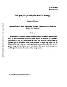
SMB = S3-brane + ΣSstrings + Sworldsheet fields +Smutual interactions , (6.22) hence one can see that the metabrane does contain both the microscopical embeddings (strings) and cosmologicalscale ones (such as our 3-brane Universe): their characteristic sizes are encoded in the corresponding weight constants αi1 ∗i2 ∗...∗ik which actually are the inverse volumes of the embeddings, like those in Eq. (6.16). When the 3-brane universe is small (the “early universe”) the value of its weight constant is comparable with those of strings and decreases as the 3-brane expands. Finally, we must say about the varieties of the formation of the string-brane world in addition to the simplest case described above, see Fig. 1 (a1). Namely, despite the transition from particle to metabrane is more or less unique due to the tough condition (6.9) or [28] for the transport matrix but: (i) it is unclear how many fundamental particles we have: for example, in the column [(b1),(b2)] of subfigures of Fig. 1 everything starts with two point particles: one particle yields strings whereas another one produces a 3-brane unlike the column [(a1),(a2)]; this question is strongly related with the total number of dimensions D: in the case [(a1),(a2)] the five strings and 3-brane can
and the latter term can be associated with the induced worldsheet curvature, V2∗D−1 λ ∂a Rν ∂b Rν ≡ Rab , V0∗D−1 4π
(6.19)
where Rab is the Ricci tensor constructed from γ˜ab , so that we eventually have the string with the induced worldsheet gravity � Z p 1 ab 0 1 γ˜ ∂a xν ∂b xν SS = − dσ dσ −˜ γ 4πα′ � λ + R , ab = 0, 1. (6.20) 4π The further generalizations can be done by analogy exploiting the decompositions (6.15) and (6.17). One 13
not have fermions, and the best way to incorporate the fermions into the picture is supersymmetry. Also, it is desirable to regard the 3-brane as the supersymmetric as well: then the bosonic coordinates are where we live in whereas the fermionic part yields the Fermi sector of the confined Standard Model. So, below we will try to perform the particle-to-fuzzyparticle-to-metabrane transition for the supersymmetric point particle in D dimensions. Let us consider the onedimensional (worldline) N = 1 supergravity [41] given by the following superspace action of the massless superparticle Z i Sp = (6.23) dθds Λ−1 ∇θ Y¯ ν ∇s Yν , 2
be incorporated into the metabrane if its worldvolume dimension is not less than 4 + 5 × 2 = 14 that in turn assumes D ≥ 14 whereas in the case [(b1),(b2)] we have the two metabranes whose worldvolume dimensions are respectively 4 and 5 × 2 = 10 (for five strings) so D must be not less than ten; (ii) the mechanism of producing of worldsheet fields is non-unique: for example, in the row [(a1),(b1)] the particle yields the metabrane which in turn produces both the desired ∗-branes and worldsheet fields on them but nothing hinders us from assuming the initial particle having the worldline field which would directly induce the worldsheet ones as drawn in the row [(a2),(b2)] rather than one uses the constructions like (6.17); (iii) the 3-brane and string are required by anthropic principle and gauge symmetry but yet there exists a lot of several ways of the split of the metabrane (6.8) (or, more precisely, (6.29)) into the ∗-branes so it is possible that 0-branes and (p 6= 3)-branes do appear as well.
where θ is the Grassmann coordinate, there is no spin connection hence the spinor covariant derivatives are ∇θ = ∂θ + iθ∂s , ∇s = ∂s ,
(6.24)
and the superfields Y and Λ are the supersymmetric counterparts of the particle’s position vector X and einbein η, respectively, Y µ = X µ + iθψ µ , Λ = η + iθχ.
(6.25) (6.26)
In the same manner as in Sec. VI A we assume that the uncertainty causes the transport also toward the directions σ i , i = 1, ..., maxdim{σ} − 1, orthogonal to the worldline: T(0) = ∂s → T = γ α ∂α ,
(6.27)
where we have taken into account our knowledge about the forthcoming Eq. (6.9) and have neglected Ref. [28] for simplicity. Also for simplicity we assume that uncertainty does not cause the transport toward extra Grassmann directions because eventually it would require the changes of the supersymmetry index N . Substituting all these formulae back into the initial action (6.23) and integrating over the Grassmann coordinate we eventually obtain the action of the fuzzy superparticle (cf. Eq. (6.7)) � Z 1 ds 1 α β Sseed = − {γ , γ }∂α X ν ∂β Xν lp η 2 � ν α β α ν ¯ (6.28) +2iψ γ ∂α ψν − iχ ¯β γ γ ∂α Xν ψ ,
FIG. 1. Some of the most characteristic ways of string-brane world formation. The dash-dotted line means subsequent applying of particle-to-fuzzy-particle “smearing” and fuzzy-particle-to-metabrane averaging procedures, the solid line means the way of how the metabrane’s worldsheet metric is decomposed; “PP”, “MB”, “3-B”, “S” mean respectively the point particle, metabrane, 3-brane, string, and “WLF” and “WSF” mean the worldline and worldsheet fields.
where we have redefined
C. Including fermions: supermetabrane
ψ → 2ψ, η −1 χ → χ ¯α γ α , η → lp η,
The scheme given in the two previous subsections is quite general but some of its components need to be corrected. Namely, everything said before holds but the strings must be supersymmetric rather than bosonic because the latter (a) do have tachyonic states, (b) do
where first Greek letters run from 0 to Dσ −1, Dσ again is the maximal number of the orthogonal directions toward which the uncertainty-caused propagation of a point particle takes place. Averaging the seed action over all the 14
deviations σ i in the spirit of Eq. (6.8), we eventually obtain the following supermetabrane action � Z √ 1 SMB = − [dσ] −γ γ αβ ∂α X ν ∂β Xν VD � ν α β α ν ¯ +2iψ γ ∂α ψν − iχ ¯β γ γ ∂α Xν ψ , (6.29)
At third (but of course not actually last), the question which is inverse to the previous one - what kind of particles corresponds to the known five (I, IIA, IIB, heterotic) strings - is also of large interest in its own. Besides, it may happen (by analogy with the quantum-mechanical Matrix theory [14]) that different strings originate from the only certain particle - this is, in fact, an alternative idea to that depicted in Fig. 1 where strings are the descendants of (meta)brane’s “decay”.
see the paragraph after Eq. (6.8) for corresponding notations. It is straightforward to check that if the conditions near Eq. (6.10) are hold (assuming the analogous ones for the fermionic part) then Eq. (6.29) yields the superstring � Z 1 0 1√ SS = − −γ γ ab ∂a X ν ∂b Xν + dσ dσ 8πα′ � (6.30) 2iψ¯ν γ a ∂a ψν − iχ ¯b γ b γ a ∂a Xν ψ ν ,
VII. CONCLUSION
Let us overview now the whole paper. As was mentioned above it can be divided into the two parts which are independent of each other for a first look. The first part (field-to-particle transition and its applications, Secs. II - IV) itself was discussed in Secs. I and V so here we will take a look on the part one only in relation to the part two. In the discussion of the first part it was conjectured that the point particle is not only the end product of field theory but also the justification of the string-brane approach. Then in the second part this conjecture was deepened: it turns out that the real point particle from the viewpoint of a macroscopic observation can look like the extended object and hence can be effectively described in terms of branes and strings. Then the 3-brane can be regarded as our Universe whereas strings describe gauge symmetry of quantum field theory. One may pictorially imagine the picture which unifies these two parts and describes the role of each of them - Fig. 2. It is doubtless that a lot of work has to be done in future. In connection with the part one: the interesting question is what is the nonminimal noninteger-spin particle. It seems that there exist two ways of how to treat it: (a) use the concept “noninteger-spin particles without spinors” [1,42], or (b) construct the models of supersymmetrical nonminimal particles. The second task is to expand the field-to-particle transition formalism on the cases of higher spacetime dimensions and more complicated fields. It seems that the whole picture holds but details may differ. In connection with the part two: we have a lot of directions for further studying and a number of unclear points, see the discussion at the bottom of Secs. VI B and VI C. Besides, there exists a number of additional questions. The first one is what is the number of dimensions of the spacetime where the fundamental particle lives. It is interesting that besides of the standard numbers 10 and 11 it was proposed (for the case of a minimal fermionic particle) the number 14 as a result of the purely spacetime realization of the symmetry group of the Standard Model SO(1, 3) × U (1) × SU (2) × SU (3) times an additional extracharge U (1) [43]. The second question is about the dualities and metabrane’s internal content. Once we try to include the strings into the one metabrane what are the
and it is clear that it is possible to repeat all the way of Sec. VI B, and eventually obtain the similar picture with the only exception: both the strings and, which is very important, 3-brane Universe do contain a fermionic sector now. Some final comments concerning the whole Sec. VI are in order. One may ask the question what are the possible applications of this viewpoint (in addition to the physically clear but abstract construction justifying the use of extended objects in field theory). It definitely hard to completely answer this question at this stage but some significance can be already outlined. At first, this formalizm can be regarded as the unique procedure which is inverse to worldvolume reduction - we start with a point-particle and obtain branes of higher dimension including strings. Therefore, one may regard the proposed approach as the realization of the worldvolume holography principle. In any case, it equips us with some kind of hierarchy (correspondence) between branes of different worldvolume dimensions. In its turn, this correspondence can be used for obtaining of valuable information about embeddings. For instance, it is well-known that strings are renormalizable at the quantum level whereas other branes are not, therefore, one may do the following: study the string (classically or non-classically) then uplift its worldvolume dimension by means of the proposed approach so that the string will not be a string anymore and becomes a brane but then a solid piece of information about the new-born brane can be obtained from string theory. At second, as was established above the simplest bosonic and fermionic particles correspond respectively to the simplest bosonic and fermionic strings. It is an exciting question what kind of strings corresponds to more complicated models of particles such as those with worldline curvature, torsion (with higher derivatives, in general), with charges of several types, curved-space corrections, etc.
15
place and role of the string-string dualities? Can they be regarded as the relations between the metabrane’s components? Also, what is the explicit internal structure of the metabrane?
[2]
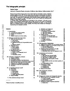
FIG. 2. Everything starts from the bare point particle; inevitable uncertainty under macroscopical measurement breaks the determinism and the particle becomes fuzzy (6.7), (6.28) from the viewpoint of a measurer; after averaging over the deviation states (in fact, this is what the procedure of a measurement does) we obtain the metabrane (6.8), (6.29) which has a varying number of worldsheet dimensions; the metabrane decays (see Fig. 1) into the superposition of ∗-branes including strings: the 3-brane yields our Universe, strings produce fields including gravity; eventually, physical field solutions after field-to-particle transition result in the nonminimal point particle(s), see Secs. II-IV. It is clear that the initial particle and the resulting one (after a cycle) are not the same - this is graphically emphasized by lens distortion, so the latter (whose action contains the higher-derivative terms) perhaps begins the new cycle. The square boxes unlike the oval ones mean the deterministic embeddings.
[3] [4] [5] [6] [7]
[8] [9]
[10]
ACKNOWLEDGMENTS
I am grateful to Edward Teo (DAMTP, Univ. of Cambridge and Natl. Univ. of Singapore) and Mikhail O. Katanaev (Steklov Math. Inst.) for helpful discussions concerning dilaton gravity and branes as well as to Belal E. Baaquie (Natl. Univ. of Singapore) for bringing some papers into my attention and for constant encouragement in superstring theory [44]. At last but not least, I acknowledge the correspondence by Mikhail S. Plyushchay (Univ. de Santiago de Chile) enlightening some subtle points of the higher-derivative particles’ mechanics.
[11]
[12] [13] [14] [15] [16]
[1] Throughout the paper by the nonminimal particle we assume the spatially 0-dimensional object whose action depends in general case on the world-line R √ curvature (rigidity) k and torsion κ: A = −µ ds x˙ ν x˙ ν F (k, κ); other historical names, “elastica” and “zero-brane”, were rejected to avoid confusing with the theory of elasticity and superembeddings, respectively. Those who wonders
[17] [18] [19] [20]
16
how a point object can possess the curvature and torsion are referred to the mathematical textbooks: B. A. Dubrovin, A. T. Fomenko and S. P. Novikov, Modern geometry - methods and applications (Springer-Verlag, New York, 1984), and Yu. Aminov, The geometry of submanifolds (Gordon and Breach, London, 1999). Here we will not consider the non-minimal terms containing the torsion (which are of higher order than those with curvature) because they are of separate large interest. B. M. Barbashov, V. V. Nesterenko and A. M. Chervyakov, Theor. Math. Phys. 40, 15 (1979); J. Phys. A 13, 301 (1980); E. Teitelboim, Phys. Lett. B 126, 41 (1983); E. d’Hoker, D. Z. Freedman and R. Jackiw, Phys. Rev. D 28, 1583 (1983); R. Jackiw and C. Teitelboim, in Quantum Theory of Gravity (Adam Hilger, Bristol, 1984). M. Ba˜ nados, C. Teitelboim, and J. Zanelli, Phys. Rev. Lett. 69, 1849 (1992). A. Ach´ ucarro and M. E. Ortiz, Phys. Rev. D 48, 3600 (1993). M. Cadoni and S. Mignemi, Phys. Rev. D 51, 4319 (1995). D. Louis-Martinez, J. Gegenberg, and G. Kunstatter, Phys. Lett. B 321, 193 (1994). H. Terao, Nucl. Phys. B 395, 623 (1993); E. Elizalde and S. Odintsov, Nucl. Phys. B 399, 581 (1993); D. Cangemi, R. Jackiw and B. Zwiebach, Ann. Phys. 245, 408 (1996); M. Cavagli´ a, V. de Alfaro and A. T. Filippov, Phys. Lett. B 424, 265 (1998). R. Rajaraman, Solitons and Instantons (North-Holland, Amsterdam, 1988). G. ’t Hooft, gr-qc/9310026; L. Susskind, J. Math. Phys. 36, 6377 (1995); E. Witten, Adv. Theor. Math. Phys. 2, 253 (1998). J. M. Maldacena, Adv. Theor. Math. Phys. 2, 231 (1998); N. Itzhaki, J. M. Maldacena, J. Sonnenschein and S. Yankielowicz, Phys. Rev. D 58, 046004 (1998). P. Claus, M. Derix, R. Kallosh, J. Kumar, P. K. Townsend and A. Van Proeyen, Phys. Rev. Lett. 81, 4553 (2000). D. Youm, Nucl. Phys. B 573, 257 (2000); Phys. Rev. D 60, 064016 (1999). M. Cadoni, P. Carta, D. Klemm and S. Mignemi, hepth/0009185; M. Cadoni and P. Carta, hep-th/0010263. T. Banks, W. Fischler, S. H. Shenker and L. Susskind, Phys. Rev. D 55, 5112 (1997). M. S. Plyushchay, Mod. Phys. Lett. A 3, 1299 (1988); Mod. Phys. Lett. A 4, 837 (1989). M. Paˇ vsiˇc, Phys. Lett. B 205, 231 (1988); Phys. Lett. B 221, 264 (1989); H. Arodz, A. Sitarz and P. Wegrzyn, Acta Phys. Polon. B 20, 921 (1989); J. Grundberg, J. Isberg, U. Lindstr¨ om and H. Nordstr¨ om, Phys. Lett. B 231, 61 (1989); J. Isberg, U. Lindstr¨ om and H. Nordstr¨ om, Mod. Phys. Lett. A 5, 2491 (1990). M. S. Plyushchay, Phys. Lett. B 253, 50 (1991). A. A. Kapustnikov, A. Pashnev, and A. Pichugin, Phys. Rev. D 55, 2257 (1997). K. G. Zloshchastiev, Phys. Rev. D 61, 125017 (2000). K. Behrndt, E. Bergshoeff, R. Halbersma and J. P. van der Schaar, Class. Quantum Grav. 16, 3517 (1999).
[41] L. Brink, P. Di Vecchia and P. Howe, Nucl. Phys. B 118, 76 (1977); J. C. Henty, P. S. Howe and P. K. Townsend, Class. Quantum Grav. 5, 807 (1988). [42] M. S. Plyushchay, Phys. Lett. B 243, 383 (1990); Phys. Lett. B 262, 71 (1991); Nucl. Phys. B 362, 54 (1991); Yu. A. Kuznetsov and M.S. Plyushchay, Nucl. Phys. B 389, 181 (1993). [43] P. Maraner, hep-th/0006109. [44] B. E. Baaquie and L. C. Kwek, NUS Lectures on Superstrings, Gauge Fields and Black Holes [hep-th/0002165].
[21] D. Louis-Martinez and G. Kunstatter, Phys. Rev. D 49, 5227 (1994); M. O. Katanaev, W. Kummer and H. Liebl, Phys. Rev. D 53, 5609 (1996); D. Youm, Phys. Rev. D 61, 044013 (2000). [22] C. G. Callan, S. B. Giddings, J. A. Harvey and A. Strominger, Phys. Rev. D 45, 1005 (1992). [23] M. O. Katanaev, W. Kummer and H. Liebl, Nucl. Phys. B 486, 353 (1997). [24] K. G. Zloshchastiev, Europhys. Lett. 49, 20 (2000); Phys. Lett. B 450, 397 (1999); Mod. Phys. Lett. A 15, 67 (2000). [25] K. G. Zloshchastiev, J. Phys. G 25, 2177 (1999). [26] J. Polchinski, String Theory (CUP, Cambridge, 1998). [27] V. A. Fock, Z. Phys. 54, 261 (1929); V. A. Fock and D. Ivanenko, Z. Phys. 54, 798 (1929); N. D. Birrell and P. C. W. Davies, Quantum fields in curved space (CUP, Cambridge, 1982), Ch. 3.8. [28] More precisely, in general case T α ’s coincide with the gamma matrices up to the scalar-field coefficient which can be associated with the square root of dilaton. If so then the physical origin of the dilaton field is deeper than it is usually regarded nowadays. [29] J. Fr¨ ohlich, O. Grandjean and A. Recknagel, Supersymmetric Quantum Theory, Non-Commutative Geometry, and Gravitation, lectures, Les Houches Summer School on Theoretical Physics, France, 1995 [hep-th/9706132]. [30] S. Deser and B. Zumino, Phys. Lett. B 65, 369 (1976); L. Brink, P. Di Vecchia and P. Howe, Phys. Lett. B 65, 471 (1976); A. M. Polyakov, Phys. Lett. B 103, 207 (1981). [31] M. J. Duff, P. S. Howe, T. Inami and K. S. Stelle, Phys. Lett. B191, 70 (1987); M. J. Duff and J. X. Lu, Nucl. Phys. B347, 394 (1990). [32] M. J. Duff, J. T. Liu and R. Minasian, Nucl. Phys. B452, 261 (1995); C. M. Hull and P. K. Townsend, Nucl. Phys. B438, 109 (1995); P. K. Townsend, Phys. Lett. B350, 184 (1995); Phys. Lett. B354, 247 (1995); C. M. Hull and P. K. Townsend, Nucl. Phys. B451, 525 (1995); E. Witten, Nucl. Phys. B443, 85 (1995). [33] J. Hughes, J. Liu and J. Polchinski, Phys. Lett. B 180, 370 (1986); E. Bergshoeff, E. Sezgin and P.K. Townsend, Phys. Lett. B 189, 75 (1987); D. Sorokin, Phys. Rep. 329, 1 (2000). [34] G. T. Horowitz and A. Strominger, Nucl. Phys. B 360, 197 (1991). [35] J. Dai, R. G. Leigh and J. Polchinski, Mod. Phys. Lett. A 4, 2073 (1989); R. G. Leigh, Mod. Phys. Lett. A 4, 2767 (1989). [36] J. Polchinski, Phys. Rev. Lett. 75, 4724 (1995); TASI Lectures on D-branes [hep-th/9611050]. [37] I. Antoniadis, N. Arkani-Hamed and S. Dimopoulos, Phys. Lett. B 436, 257 (1998) [hep-ph/9804398]; N. Arkani-Hamed, S. Dimopoulos and G. Dvali, Phys. Rev. D 59, 086004 (1999) [hep-ph/9807344]. [38] M. Gogberashvili, hep-ph/9812296; Europhys. Lett. 49, 396 (2000) [hep-ph/9812365]. [39] L. Randall and R. Sundrum, Phys. Rev. Lett. 83, 4690 (1999) [hep-th/9906064]; Phys. Rev. Lett. 83, 3370 (1999) [hep-ph/9905221]. [40] K. G. Zloshchastiev, gr-qc/0007075 (submitted to Class. Quantum Grav.).
17