Holography for Cosmology Paul McFadden∗ and Kostas Skenderis† Institute for Theoretical Physics, Valckenierstraat 65, 1018XE Amsterdam. (Dated: Jan 13, 2010)
arXiv:0907.5542v2 [hep-th] 13 Jan 2010
We propose a holographic description of four-dimensional single-scalar inflationary universes, and show how cosmological observables, such as the primordial power spectrum, are encoded in the correlation functions of a three-dimensional quantum field theory (QFT). The holographic description correctly reproduces standard inflationary predictions in the regime where a perturbative quantization of fluctuations is justified. In the opposite regime, wherein gravity is strongly coupled at early times, we propose a holographic description in terms of perturbative large N QFT. Initiating a holographic phenomenological approach, we show that models containing only two parameters, N and a dimensionful coupling constant, are capable of satisfying the current observational constraints. PACS numbers: 11.25.Tq, 98.80.Cq
Introduction. Over the last two decades striking new observations have transformed cosmology from a qualitative to quantitative science. A minimal set of cosmological parameters characterizing the observed universe, the concordance cosmology, have now been measured to within a few percent [1]. These observations reveal a spatially flat universe, endowed with small-amplitude primordial perturbations that are approximately Gaussian and adiabatic with a nearly scale-invariant spectrum. These findings are consistent with the generic predictions of inflationary cosmology and set inflation as the leading theoretical paradigm for the initial conditions of Big Bang cosmology. With future observations promising an unprecedented era of precision cosmology, the constraints on cosmological parameters are expected to tighten further still, particularly as regards the inflationary sector. This presents a unique window to Planck-scale physics and a challenge for fundamental theory. During the last decade we have also witnessed exciting new developments in fundamental theory. Holographic dualities have been proposed and developed leading to a new viewpoint for physical reality. Holography states that any quantum theory of gravity should have a description in terms of a quantum field theory (QFT) which does not contain gravity in one dimension less. It is natural to wonder how cosmology fits into the holographic framework and the main aim of this article is to propose a concrete holographic framework for inflationary cosmology. Apart from the conceptual advances that such a development would imply, there are also a number of more pragmatic reasons for developing such a framework. Firstly, uncovering the structure of three-dimensional QFT in cosmological observables brings in new intuition about their structure and may lead to more efficient computational techniques, cf. the computation of non-Gaussianities in [2]. Secondly, holographic dualities are strong/weak coupling dualities meaning that in the regime where the one description is weakly coupled the other is strongly coupled. This provides an arena for
constructing new models with intrinsic strong-coupling gravitational dynamics at early times that have only a weakly coupled three-dimensional QFT description and are thus outside the class of model described by standard inflation. Such models may well lead to qualitatively different predictions for the cosmological observables that will be measured in the near future. Any holographic proposal should specify what the dual QFT is and how to use it to compute cosmological observables. The holographic description we propose uses the one-to-one correspondence between cosmologies and domain-wall spacetimes discussed in [3, 4] and assumes that the standard gauge/gravity duality is valid. More precisely, the steps involved are illustrated in Fig. 1. The first step is to map any given inflationary model to a domain-wall spacetime. For inflationary cosmologies that at late times approach either a de Sitter spacetime or a power-law scaling solution [5], the corresponding domain-wall solutions describe holographic renormalization group flows. For these cases there is an operational gauge/gravity duality, namely one has a dual description in terms of a three-dimensional QFT. Now, the map between cosmologies and domain-walls can equivalently be expressed entirely in terms of QFT variables, and amounts to a certain analytic continuation of parameters and momenta. Applying this analytic continuation we obtain the QFT dual of the original cosmological spacetime. We shall call the resulting theory a ‘pseudo’-QFT because we currently only have an operational definition of this theory. Namely, we do the computations in the QFT theory dual to the corresponding domain-wall and then apply the analytic continuation. Perhaps a more fundamental perspective is to consider the QFT action, with complex parameters and complex fields as the fundamental objects, and then to consider the results on different real domains as applicable to either domain-walls or cosmologies. Note that the supergravity embedding of the domain-wall/cosmology correspondence discussed in [6] works in precisely this way.
2 lution of the scalar field is (piece-wise) monotonic, ϕ(z) can be inverted to give z(ϕ), allowing the Hubble rate H = a/a ˙ to be expressed in terms of some ‘fake superpotential’ W (ϕ) as H(z) = −(1/2)W (ϕ). The complete equations for the background are then 1 a˙ = − W, a 2
FIG. 1: The ‘pseudo’-QFT dual to inflationary cosmology is operationally defined using the correspondence of cosmologies to domain-walls and standard gauge/gravity duality.
The holographic description should reproduce standard inflationary results in their regime of applicability, namely when the fluctuations around the cosmological background can be perturbatively quantized. New results should follow by applying the duality in the cases where such a perturbative quantization of fluctuations is not justified. In the remainder of this article, we show first that the standard results are indeed reproduced, then move to construct new models which are strongly coupled at early times but have a weakly coupled large N QFT description. Domain-wall/cosmology correspondence. For simplicity, we focus on spatially flat universes equipped with a single minimally coupled scalar field, but the results can be extended to more general cases (eg., non-flat, multiscalar, non-canonical kinetic terms, etc.) The linearly perturbed metric and scalar field may be written in the form ds2 = ηdz 2 + a2 (z)[δij + hij (z, ~x)]dxi dxj , Φ = ϕ(z) + δϕ(z, ~x),
(1)
where η = −1 in the case of cosmology, in which case z is the time coordinate, and η = +1 in the case of domain-wall solutions, in which case z is the radial coordinate. We take the domain-wall to be Euclidean for later convenience. A Lorentzian domain-wall may be obtained by continuing one of the xi coordinates to become the time coordinate [4]. The continuation to a Euclidean domain-wall is convenient, however, because the QFT vacuum state implicit in the Euclidean formulation maps to the Bunch-Davies vacuum on the cosmology side. Other choices of cosmological vacuum require considering the boundary QFT in different states, as may be accomplished using the real-time formalism of [7]. The actions for both the cosmology and the Euclidean domain-wall may be written in the combined form Z p η (2) S = 2 d4 x |g| [−R + (∂Φ)2 + 2κ2 V (Φ)], 2κ where κ2 = 8πG and we take the scalar field Φ to be dimensionless. For background solutions in which the evo-
ϕ˙ = W ′ ,
3 2ηκ2 V = W ′2 − W 2 , 2
(3)
where W ′ = dW/dϕ. This first-order formalism goes back to the work of [8] (for cosmology), where it was obtained by application of the Hamilton-Jacobi method. In [4] this formalism was linked to the notion of (fake) (pseudo-) supersymmetry. The equations of motion for the perturbations are 0 = ζ¨ + (3H + ǫ/ǫ) ˙ ζ˙ − ηa−2 q 2 ζ, 0 = γ¨ij + 3H γ˙ ij − ηa−2 q 2 γij ,
(4)
where ~q is the comoving wavevector of the perturbations, and the background quantity ǫ(z) is defined as 2 ˙ ǫ = −H/H = 2(W ′ /W )2 . γij is a transverse traceless metric perturbation and ζ = ψ + (H/ϕ)δϕ ˙ is the standard gauge-invariant variable constructed from a metric perturbation, hij = −2ψ(z, ~x)δij , and the scalar perturbation δϕ. Defining now the analytically continued variables κ ¯ and q¯ according to κ ¯ 2 = −κ2 ,
q¯ = −iq ,
(5)
it is easy to see that a perturbed cosmological solution written in terms of the variables κ and q continues to a perturbed Euclidean domain-wall solution expressed in terms of the variables κ ¯ and q¯. We have thus established that the correspondence between cosmologies and domain-walls holds, not only for the background solutions, but also for linear perturbations around them. This is the basis for the relation between power spectra and holographic 2-point functions, to be discussed momentarily. The argument can be generalized to arbitrary order to relate non-Gaussianities to holographic higher-point functions [9]. Quantization of perturbations. In the inflationary paradigm, cosmological perturbations originate on subhorizon scales as quantum fluctuations of the vacuum. Quantizing the perturbations in the usual manner, one finds the scalar and tensor superhorizon power spectra q3 q3 hζ(q)ζ(−q)i = |ζq(0) |2 , 2 2π 2π 2 2q 3 q3 hγ (q)γ (−q)i = |γq(0) |2 , ∆2T (q) = ij ij 2π 2 π2 ∆2S (q) =
(6)
where γq(0) and ζq(0) are the constant late-time values of the cosmological mode functions γq (z) and ζq (z). The mode functions are themselves solutions of the classical equations of motion (4) (setting γij = γq eij , for
3 some time-independent polarization tensor eij ). To select a unique solution for each mode function we impose the Bunch-Davies vacuum condition ζq , γq R ∼ e−iqτ as z τ → −∞, where the conformal time τ = dz ′ /a(z ′ ). The normalization of each solution (up to an overall phase) may then be fixed by imposing the canonical commutation relations for the corresponding quantum fields. This leads to the Wronskian conditions, ∗ i = ζq Π(ζ)∗ − Π(ζ) q q ζq ,
i/2 = γq Π(γ)∗ − Πq(γ) γq∗ , q
(7)
(γ) (ζ) where Πq = 2ǫa3 κ−2 ζ˙q and Πq = (1/4)a3 κ−2 γ˙ q are the canonical momenta associated with each mode function, and we have set ~ to unity. To make connection with the holographic analysis to follow, we introduce the linear response functions E and Ω satisfying
Π(ζ) q = Ω ζq ,
Πq(γ) = E γq .
(8)
(These quantities are well-defined since we have already selected a unique solution for each mode function). Substituting these definitions into the Wronskian conditions, which are valid at all times, the cosmological power spectra may be re-expressed as ∆2S (q) =
−q 3 , 4π 2 ImΩ(0) (q)
∆2T (q) =
−q 3 , (9) 2π 2 ImE(0) (q)
where ImΩ(0) and ImE(0) are the constant late-time values of the imaginary part of the response functions. We will see shortly how the response functions also give the 2-point functions of the pseudo-QFT. Let us now consider the corresponding domain-wall solution obtained by the applying the continuation (5). The early-time behavior ∼ e−iqτ of the cosmological perturbations maps to the exponentially decaying behavior ∼ eq¯τ in the interior of the domain-wall (τ → −∞). Such regularity in the interior is a prerequisite for holography, explaining our choice of sign in the continuation of q. ¯ and Ω ¯ [10] are The domain-wall response functions E defined analogously to (8), namely ¯ ¯ (ζ) Π q¯ = −Ω ζq¯
¯ ¯ (γ) Π q¯ = −E γq¯,
(10)
¯ (γ) ¯ (ζ) = (1/4)a3 κ ¯ −2 γ˙ q¯ are = 2ǫa3 κ ¯−2 ζ˙q¯ and Π where Π q¯ q¯ the radial canonical momenta. The minus signs are in¯ ¯ serted so that Ω(−iq) = Ω(q) and E(−iq) = E(q). By choosing the arbitrary overall phase of the cosmological perturbations appropriately, we may ensure that the domain-wall perturbations are everywhere real. The domain-wall response functions are then purely real, while their cosmological counterparts are complex. Holographic analysis. There are two classes of domain-wall solutions for which holography is well understood.
(i) Asymptotically AdS domain-walls. solution behaves asymptotically as a(z) ∼ ez ,
ϕ∼0
as
In this case the
z → ∞.
(11)
The boundary theory has a UV fixed point which corresponds to the bulk AdS critical point. Depending on the rate at which ϕ approaches zero as z → ∞, the QFT is either a deformation of the CFT or else the CFT in a state in which the dual scalar operator acquires a nonvanishing vacuum expectation value (see [11] for details). Under the domain-wall/cosmology correspondence, these solutions are mapped to cosmologies that are asymptotically de Sitter at late times. (ii) Asymptotically power-law solutions. In this case the solution behaves asymptotically as √ a(z) ∼ (z/z0 )n , ϕ ∼ 2n log(z/z0 ) as z → ∞, (12) where z0 = n−1. This case has only very recently been understood [12]. For n = 7 the asymptotic geometry is the near-horizon limit of a stack of D2 brane solutions. In general, these solutions describe QFTs with a dimensionful coupling constant in the regime where the dimensionality of the coupling constant drives the dynamics. Under the domain-wall/cosmology correspondence, these solutions are mapped to cosmologies that are asymptotically power-law at late times. Holographic 2-point functions are now obtained by solving the linearized equations of motion about the domain-wall solution with Dirichlet boundary conditions at infinity and imposing regularity in the interior. It will suffice to discuss the 2-point function for the energymomentum tensor. On general grounds, the 2-point function takes the form hTij (¯ q )Tkl (−¯ q )i = A(¯ q )Πijkl + B(¯ q )πij πkl ,
(13)
where Πijkl is the three-dimensional transverse traceless projection operator defined by Πijkl = πi(k πl)j −(1/2)πij πkl and πij = δij −¯ qi q¯j /¯ q 2 . The holographic computation amounts to the extracting the coefficients A and B from the asymptotics of the linearized solution. Using the radial Hamiltonian method developed in [10], one finds ¯(0) (¯ A(¯ q ) = 4E q ),
B(¯ q) =
1¯ Ω(0) (¯ q ), 4
(14)
where the zero subscript indicates the leading (constant) term as z → ∞, after holographic renormalization has been performed [10, 13]. Continuation to the pseudo-QFT. We now wish to re-express the bulk analytic continuation (5) in terms of QFT variables. This amounts to ¯ 2 = −N 2 , N
q¯ = −iq,
(15)
4 where the barred quantities are associated with the QFT dual to the domain-wall. We thus find that the power spectrum for any inflationary cosmology that is asymptotically de Sitter or asymptotically power law can be directly computed from the 2-point function of a threedimensional QFT via the formulae: ∆2S (q) =
−q 3
16π 2 ImB(−iq)
, ∆2T (q) =
−2q 3
π 2 ImA(−iq)
. (16)
Beyond the weak gravitational description. In the discussion so far we have assumed that the description in terms of gravity coupled to a scalar field is valid at early times, and that the perturbative quantization of fluctuations can be justified. The holographic description also allows us to obtain results when these assumptions do not hold. At early times, the theory may be strongly coupled with no useful description in terms of low-energy fields (such as the metric and the scalar field). The holographic set-up allows us to extract the late-time behavior of the system, which can be expressed in terms of lowenergy fields, from QFT correlators. (For further details see [13]). Here we only note that this is the counterpart of the standard fact that in gauge/gravity duality the asymptotic behavior of bulk fields near the boundary of spacetime is reconstructed by the correlators of the dual QFT [14]. This late-time behavior is precisely the information we need to compute the primordial power spectra and other cosmological observables. Ideally one would deduce from a string/M-theoretic construction what the dual QFT is. Instead we initiate here a holographic phenomenological approach. The dual QFT would involve scalars, fermions and gauge fields and it should admit a large N limit. The question is then whether one can find a theory which is compatible with current observations. In particular, one might consider either deformations of CFTs or theories with a single dimensionful parameter, as these QFTs have already featured in our discussion above. We will discuss here super-renormalizable theories that contain one dimensionful coupling constant. A prototype example is SU (N ) Yang-Mills theory coupled to a number of scalars and fermions, all in the adjoint of SU (N ). To extract predictions we need to compute the coefficients A and B of the 2-point function of the energymomentum tensor (13), analytically continue the results and insert them in the holographic formulae for the power spectra. Firstly, the leading contribution to the 2-point function of the energy-momentum tensor is at one loop. Since the energy-momentum tensor has dimension three, ¯ 2 q¯3 , A(¯ q) ∼ N
¯ 2 q¯3 . B(¯ q) ∼ N
(17)
A generic such model thus leads to a scale-invariant spectrum at leading order in N . To fix the parameters of these
FIG. 2: The straight line is the leading order prediction of holographic models with a single dimensionful coupling constant for the correlation of the running αs and the scalar tilt ns . The data show the 68% and 95% CL constraints (marginalizing over tensors) at q = 0.002 Mpc−1 , and are taken from Fig. 4 of [1]. As new data appear the allowed region should shrink to a point, which is predicted to lie close to the line.
models we may then compare with observations. Comparing the observed amplitude of the scalar power spectrum [1] with its holographic value we find N ∼ O(104 ), justifying the large N limit. To determine the coupling 2 constant gYM we may compare with the tilt of the spectrum. The precise formula requires a two-loop computation [16] and will be reported elsewhere [9]. One can obtain an order of magnitude estimate, however, on general grounds. The perturbative expansion depends on the 2 2 ¯ /¯ effective dimensionless coupling constant geff = gYM N q, and the leading correction to the 2-point function yields 2 (ns −1) = cgeff , where the constant c is of order one and depends on the details of the theory. From Table 4 of [1] one finds that (ns −1) ∼ O(10−2 ), thus we find that 2 ∼ O(10−2 ) justifying the perturbative QFT treatgeff ment. Independently of the details of the theory, the 4 scalar index runs: αs = dns /d ln q = −(ns −1) + O(geff ). This prediction is qualitatively different from slow-roll inflation (for which αs /(ns −1) is of first-order in slow-roll [18]), yet is nonetheless consistent with the constraints on ns and αs given in [1] for a wide range of values of ns and αs , as illustrated in Fig. 2. The ratio of tensor to scalar power spectra can be computed from (16), yielding r = 32ImB(−iq)/ImA(−iq). For massless scalars and for ¯ 2q¯3 (for conformally couvector fields A = B = (1/256)N pled scalars B = 0 instead), and for massless fermions ¯ 2q¯3 and B = 0. With appropriate field A = (1/128)N content one can thus satisfy the current observational bound on r. 2 Once N , gYM and the field content are fixed, all other cosmological observables (such as non-Gaussianities, etc.) follow uniquely from straightforward computa-
5 tions. We will present details of the correspondence between higher-order QFT correlation functions and nonGaussian cosmological observables elsewhere [9]. Our results indicate, however, that the non-Gaussianity palocal rameter fN L [15] is independent of N to leading order, consistent with current observational evidence [1]. Conclusions. We have presented a concrete proposal describing holography for cosmology, and initiated a holographic phenomenological approach capable of satisfying current observational constraints. Clearly one would like to further develop holographic phenomenology and obtain precise predictions for the cosmological observables to be measured by forthcoming experiments. We hope to report on this in the near future. Acknowledgements. We thank NWO for support.
∗ †
[1] [2] [3] [4] [5]
[email protected] [email protected] E. Komatsu et al. (WMAP), Astrophys. J. Suppl. 180, 330 (2009), arxiv:0803.0547. J. Maldacena, JHEP 05, 013 (2003), astro-ph/0210603. M. Cvetic and H. H. Soleng, Phys. Rev. D51, 5768 (1995), hep-th/9411170. K. Skenderis and P. K. Townsend, Phys. Rev. Lett. 96, 191301 (2006), hep-th/0602260; J. Phys. A40, 6733 (2007), hep-th/0610253. This era should then be followed by a hot big bang cosmology, as in standard discussions. Here we only discuss the very early universe, i.e., the times when the primordial cosmological perturbations were generated (the in-
flationary epoch). [6] E. A. Bergshoeff, J. Hartong, A. Ploegh, J. Rosseel and D. van den Bleeken, JHEP 07, 067 (2007), arxiv:0704.3559; K. Skenderis, P. K. Townsend and A. van Proeyen, JHEP 08, 036 (2007), arxiv:0704.3918. [7] K. Skenderis and B. C. van Rees, Phys. Rev. Lett. 101, 081601 (2008), arxiv:0805.0150. [8] D. S. Salopek and J. R. Bond, Phys. Rev. D42, 3936 (1990). [9] P. McFadden and K. Skenderis, to appear. [10] I. Papadimitriou and K. Skenderis, JHEP 10, 075 (2004), hep-th/0407071. [11] K.Skenderis, Class. Quant. Grav. 19, 5849 (2002), hepth/0209067. [12] I. Kanitscheider, K. Skenderis and M. Taylor, JHEP 09, 094 (2008), arxiv:0807.3324. [13] P. McFadden and K. Skenderis, arxiv:1001.2007. [14] S. de Haro, S. N. Solodukhin and K. Skenderis, Commun. Math. Phys. 217, 595 (2001), hep-th/0002230. [15] E. Komatsu and D. N. Spergel, Phys. Rev. D63, 063002 (2001), astro-ph/0005036. [16] Super-renormalizable theories have infrared divergences, but large N resummation leads to well-defined expres2 sions with gYM effectively playing the role of an infrared regulator. The exact amplitudes are nonanalytic functions of the coupling constant [17]. Note that our analytic continuation to pseudo-QFT does not involve the coupling constant. [17] R. Jackiw and S. Templeton, Phys. Rev. D23, 2291 (1981); T. Appelquist and R. D. Pisarski, Phys. Rev. D23, 2305 (1981). [18] A. Kosowsky and M. Turner, Phys. Rev. D52, 1739 (1995), astro-ph/9504071.