homotopy method for the large sparse real nonsymmetric ... - CiteSeerX

HOMOTOPY METHOD FOR THE LARGE SPARSE REAL NONSYMMETRIC EIGENVALUE PROBLEM S. H. LUI , H. B. KELLER y , AND T. W. C. KWOKz

Abstract. A homotopy method to compute the eigenpairs, i.e., the eigenvectors and eigenvalues, of a given real matrix A1 is presented. From the eigenpairs of some real matrix A0 , the eigenpairs of A(t)  (1 ? t)A0 + tA1 are followed at successive \times" from t = 0 to t = 1 using continuation. At t = 1, the eigenpairs of the desired matrix A1 are found. The following phenomena are present when following the eigenpairs of a general nonsymmetric matrix:  bifurcation  ill-conditioning due to non-orthogonal eigenvectors  jumping of eigenpaths These can present considerable computational diculties. Since each eigenpair can be followed independently, this algorithm is ideal for concurrent computers. The homotopy method has the potential to compete with other algorithms for computing a few eigenvalues of large sparse matrices. It may be a useful tool for determining the stability of a solution of a PDE. Some numerical results will be presented. Key words. eigenvalues, homotopy, parallel computing, sparse matrices, bifurcation AMS subject classi cations. 65F15, 65H17

1. Introduction. Given a real n  n matrix A, we wish to nd some or all its eigenvalues and eigenvectors. That is, we seek  2 CI such that Ax = x holds for nontrivial x 2 CI n . We call (x; ) an eigenpair. The QR algorithm (see Golub and van Loan [9]) is generally regarded as the best sequential method for computing the eigenpairs. Brie y, the QR algorithm uses a sequence of similarity transformations to reduce a matrix to upper Hessenberg form. It then applies a sequence of Givens rotations from the left and right to reduce the size of the sub-diagonal elements. When these elements are suciently small, the diagonal elements are taken to be approximations to the eigenvalues of the matrix. If the matrix is large and sparse, the QR algorithm suers two serious drawbacks. In the reduction to Hessenberg form, the matrix usually loses its sparsity. Hence the  Hong Kong University of Science & Technology, Department of Mathematics, Clear Water Bay, Kowloon, Hong Kong. This work was in part supported by RGC grant DAG92/93.SC16. y California Institute of Technology, 217-50, Pasadena, CA 91125. z Hong Kong University of Science & Technology, Department of Mathematics, Clear Water Bay, Kowloon, Hong Kong. 1

algorithm requires the explicit storage of the entire matrix. This may pose a problem if the matrix is so large that not all its entries can be accommodated within the main memory of the computer. A second drawback is that it is inherently a sequential algorithm due to the fact that Givens rotations must be applied sequentially. Bai and Demmel [3] have circumvented somewhat the second problem by performing a \block" version of the QR algorithm. This improved version seems to work well on vector machines. We now describe a homotopy method to compute the eigenpairs of a given matrix

A1 . From the eigenpairs of some real matrix A0 , we follow the eigenpairs of A(t)  (1 ? t)A0 + tA1 at successive times from t = 0 to t = 1 using continuation. At t = 1, we have the eigenpairs of the desired matrix A1 . We call the evolution of an eigenpair as a function of time an eigenpath. When A1 is a real symmetric tridiagonal matrix with nonzero o-diagonal elements, a very successful homotopy method is known (see Li and Li [16] and Li, Zhang and Sun [21]). The following phenomena, while absent in the symmetric tridiagonal case, are present for the general case:

 bifurcation  ill-conditioning due to non-orthogonal eigenvectors The rst can present computational diculties if not handled properly. The homotopy method does not produce the Schur decomposition. Instead, it evaluates the eigenvalues and eigenvectors and hence is subject to the diculty of ill-conditioning. Since the eigenpairs can be followed independently, this algorithm is ideal for parallel computers. We are primarily concerned with the case of a large, sparse, real matrix. We assume that all the nonzero entries of the matrix can be stored in each node of a parallel computer with distributive memory. Furthermore, we assume that the associated linear systems can be solved quickly, say in O(n2 ) time. 2

I



0

1

t II



0

1

t III



0

1

t

. Eigenpaths of a 2 by 2 matrix. The dotted lines denote complex eigenpaths.

Fig. 1

As a simple illustration, we consider 22 matrices where the matrix A0 is diagonal whose elements are the diagonal elements of A1 : 







A0 = a0 0b ; A1 = ac db : 3

The eigenvalues of A(t) are

p

a + b  (a ? b)2 + 4t2 cd : 2

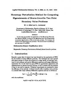
Assuming a 6= b, then three dierent situations arise (see Figure 1). In the rst case, the two eigenvalues never meet for all t in [0; 1]. In the second case, there is a double eigenvalue at some time t 2 (0; 1] with the eigenpaths remaining real throughout. In the third case, there is a bifurcation point with the eigenpaths becoming a complex conjugate pair to the right of the bifurcation point. Typically this is how complex eigenpaths arise from real ones. (Whenever a quantity is said to be complex, we mean it has a nontrivial imaginary component.) The situation for higher dimensional matrices is similar except that an eigenpath can have more than one bifurcation point and that the reverse of case three described above can occur (i.e., complex conjugate pair of eigenpaths occur to the left of the bifurcation point and two real eigenpaths to the right.) See Figure 2 for the eigenpaths of a random 10 by 10 matrix. We now give a synopsis of the rest of the paper. In Section 2, the homotopy method along with complex bifurcations will be presented. We will discuss some dierent types of bifurcations that may arise and identify the generic kind. We will derive an upper bound on the number of bifurcation points of all the eigenpaths. The numerical algorithm will be discussed in Section 3. We will describe how to deal with bifurcations, how to choose the initial matrix, the selection of stepsizes etc.. This will be followed by some numerical results. We will see that our homotopy method is impractical for dense matrices but has the potential to compete with other algorithms for nding a few eigenvalues of large sparse matrices. Matrices of dimension 104 arising from the discretization of PDEs have been tested. In the nal section, we recapitulate and suggest directions of further research. Li, Zeng and Cong [20] and Li and Zeng [19] have a very ecient homotopy method for the dense matrix eigenvalue problem. For other approaches to the nonsymmetric eigenvalue problem, see for example, Cullum and Willoughby [5], Dongarra 4

3.5

'real' 'complex'

3 2.5 2 1.5



1 0.5 0 -0.5 -1 -1.5

0

0.2

0.4

t

0.6

0.8

Fig. 2. Eigenpaths of a random 10 by 10 matrix. Only one path of a complex conjugate pair of eigenpaths is shown.

and Sidani [6], Saad [25], Shro [28], Sorensen [29], Ruhe [24] and Bai et al [2]. The classic reference for the eigenvalue problem is the treatise by Wilkinson [30]. See also Saad [26] and Bai and Demmel [4] and references therein. Except for some of the numerical results, the work in this paper had been completed in Lui [22]. In the paper of Li, Zeng and Cong [20], they prove Lemma A.1 5

1

(which they attribute to an unpublished work of H. B. Keller) which gives a necessary condition for a certain quantity (  (G0uu 2 )) to be nonzero. In this paper (Theorem 2), we give a necessary as well as sucient condition. Using analytic bifurcation theory, we identify the generic kinds of bifurcation which occur in following eigenpaths. We also give a bound on the number of bifurcation points in the eigenpaths. While the paper of Li et al address the dense eigenvalue problem, we address the complementary sparse case though our algorithm has not had the same degree of success as theirs.

2. Homotopy Method and Complex Bifurcation. In this section, we discuss some of the various phenomena that may arise on an eigenpath. Usually an eigenpath will be locally unique. That is, there are no other eigenpaths nearby. This can be characterized by a certain Jacobian being nonsingular. When this Jacobian is singular, bifurcation may occur. In other words, two or more eigenpaths may intersect at a point (u0 ; t0 ). Applying Henderson's work [10] on general analytic equations to our eigenvalue equations, we give a partial classi cation of some of the possible cases: simple quadratic fold, simple bifurcation point, simple cubic fold and simple pitchfork bifurcation. We will show that the generic kind of bifurcation is the simple quadratic fold. In fact, the transition between real and complex eigenpaths (and vice versa) are via simple quadratic folds. We rst establish some notation. We use the superscripts T and  to denote the transpose and the complex conjugate transpose respectively. The null and range spaces of a matrix are written as N () and R() respectively. The ith column of the identity matrix I is denoted by ei . Given a real n  n matrix A1 , we form the homotopy (1)

A(t) = (1 ? t)A0 + tA1 ; 0  t  1; 6

where A0 is a real matrix. We write the eigenvalue problem of A(t) as: 



G(u; t)  A(tn)x(x?) x = 0;

(2)

where u is the eigenpair (x; ) of A(t) and n(x) is a normalization equation. In this paper, we take

n(x) = c x ? 1; where c is some xed vector that is not orthogonal to x. The usual normalization

n(x)  x x ? 1 is not dierentiable except at x = 0 and it only de nes x up to a complex constant of magnitude one. We will always assume that every eigenvector x satis es c x 6= 0; in section 3, we show how to choose c . At this point, we make some remarks concerning the homotopy. It is known (Kato [12]) that the eigenvalues of A(t) are analytic functions of t except at nitely many points where some eigenvalue may have an algebraic singularity. Away from these singularities, the eigenvectors can be chosen to be analytic functions of t. As we shall see, typically, these singularities are encountered when an eigenvalue makes the transition from real to complex or vice versa. Suppose an eigenpair u0 is known at time t0 , i.e., G(u0 ; t0 ) = 0: We now describe how to obtain an eigenpair at a later time t1 . We must separate the discussion into dierent cases, depending on whether the Jacobian G0u  Gu (u0 ; t0 ) is singular or not and on the nature of the singularity.

2.1. Nonsingular Jacobian. When G0u is nonsingular, then the Implicit Function Theorem tells us that locally about t0 , there is a unique solution u(t) with u(t0 ) = u0 . Dierentiating (2) with respective to t and evaluating at t0 , we obtain

G0u u_ 0 + G0t = 0; where dot denotes t derivative and G0t  Gt (u0 ; t0 ). Since G0u is nonsingular, the above equation has a unique solution u_ 0. To obtain the eigenpair at a later time t1 , we 7



:o u_ 0

o

t0

0

t

t1

1

. Euler-Newton continuation

Fig. 3

apply Newton's Method to the equation G(u; t1 ) = 0 with initial guess u0 +(t1 ? t0 )u_ 0 . This is the Euler-Newton continuation method. The Euler step (t1 ? t0 )u_ 0 is used to obtain the rst Newton iterate (see Figure 3). Provided t1 ? t0 is suciently small, the Newton iterates will converge quadratically to the eigenpair at t1 .

2.2. Singular Jacobian: Simple Quadratic Fold. Here we assume the eigenpair u0 is real and

 G0u has a one-dimensional null space spanned by say , and let span the null space of G0uT ,

 G0t 62 R(G0u ),  a  T (G0uu 2 ) 6= 0. Note that G0uu 2 is a shorthand for G0uu . The point (u0 ; t0 ) having the above properties is said to be a simple (real) quadratic fold point of Equation 2. Pictorially, the real eigenpath is represented as the solid curve in Figure 4. Later, we will see that an equivalent de nition is that (1) 0 is an eigenvalue of A(t0 ) with algebraic multiplicity two and geometric multiplicity one, and (2) A0 (t0 )x0 is not in the range of [A(t0 ) ? 0 I; ?x0 ].

8



6 U



0

i 1

t

Fig. 4. Complex conjugate pair of solutions on the opposite side of a simple real quadratic fold point. Dotted lines denote complex solutions.

Since we can no longer use t to parametrize the solution, we employ the following pseudo-arclength method due to Keller [13]. Augment (2) with the scalar equation:

g(u; t; s)  T
(u ? u0) ? (s ? s0 ) = 0: This is the equation of a hyperplane whose normal is  and is at a distance s ? s0 from u0 . Now de ne (3)





F (u; t; s)  Gg :

We have immediately F (u0 ; t0 ; s0 ) = 0. It can be shown that the derivative of F with respect to (u; t) and evaluated at (u0 ; t0 ; s0 ) (4)

F(0u;t) =



G0u G0t T 0



is nonsingular. Hence again by the Implicit Function Theorem, F has a locally unique solution (u(s); t(s); s) with u(s0 ) = u0 and t(s0 ) = t0 . In fact, the solution has the form:

u(s) = u0 + (s ? s0 ) + O(s ? s0 )2 ; (5)

t(s) = t0 +  (s ? s0 )2 + O(s ? s0 )3 ;

where

 = ? 21

T (G0 2 ) uu  G0t : 9

From the de nition of a simple quadratic fold,  is well-de ned and nonzero. Note that dt(s0 )=ds = 0. We can apply the Euler-Newton continuation to the system F = 0 and follow the eigenpath around the fold point. Geometrically, the solution of F = 0 is the point at which the eigenpath punctures the hyperplane g = 0. Once around the fold point, t will begin to decrease. This is undesirable since our goal is to compute the eigenpair at t = 1. It turns out that a complex conjugate pair of eigenpaths will emerge to the right of the fold point. We now elaborate on this point. Recall that a point P0  (u0 ; t0 ) is called a bifurcation point of the equation

G(u; t) = 0 if in a neighborhood of P0 , there are at least two distinct branches of solutions (u1 (s); t1 (s)) and (u2 (s); t2 (s)) such that ui (s0 ) = u0 and ti (s0 ) = t0 for i = 1; 2: If at least one of these branches is complex, we will call P0 a complex bifurcation point. When u0 is real, (2) is a system of real equations. From the last paragraph, we know that locally about the point P0 , there is a unique path of real solutions. However, when considered as a system of equations over the complex

numbers, Henderson and Keller [11] have shown that P0 is a complex bifurcation point with a complex conjugate pair of solutions on the opposite side of the real quadratic fold (see Figure 4). Furthermore, the complex solutions have local expansions:

u(s) = u0 + i(s ? s0 ) + O(s ? s0 )2 ; t(s) = t0 ?  (s ? s0 )2 + O(s ? s0 )3 : They are very similar in form to the real solution (5). Note that the tangent vector of the complex solution is a rotation of the tangent () of the real solution. We can now use the Euler-Newton continuation with initial step in the direction i to nd the complex eigenpairs at a later time. The result of Henderson and Keller can be generalized to a complex quadratic fold point: i.e., u0 2 CI n+1 and satis es the three properties outlined at the beginning of this section.

10

Theorem 1 (Henderson [10]). Let G(u; t) be an analytic operator from CI n+1  IR to CI n+1 . Let (u0; t0) be a simple quadratic fold point of G(u; t) = 0. Then

in a small neighborhood of (u0 ; t0 ), there exist exactly two solution branches. They have the expansions for small jj:

u1() = u0 + e?i=2  + O(2 ); t1 () = t0 ? r2 + O(3 ); u2() = u0 + ie?i=2 + O(2 ); t2 () = t0 + r2 + O(3 ); where  0 2 rei = 2(GuuG0 ) : t

2.3. Singular Jacobian: Simple Quadratic Bifurcation. Here, we assume the eigenpair u0 is real and,

 G0u has a one-dimensional null space spanned by say , and let span the null space of G0uT ,

 G0t 2 R(G0u ),  a= 6 0 and b2 ? ac 6= 0, where a = T (G0uu 2 ); b = T (G0uu 0 + G0ut ); c = T (G0uu 20 + 2G0ut 0 ); and 0 is the unique solution of (6) orthogonal to N (G0u ).

G0u 0 = ?G0t 11

The point (u0 ; t0 ) having the above properties is called a simple quadratic bifurcation point. In any small neighborhood of (u0 ; t0 ), there are exactly two distinct branches of solutions passing through the point (u0 ; t0 ) transcritically. If b2 ? ac > 0, then both branches are real. If b2 ? ac < 0, both branches are complex except at the point (u0 ; t0 ). See Henderson [10] for a more detailed discussion. The tangent vectors of the two bifurcating branches can be computed and the Euler-Newton continuation can proceed as usual with these new directions. We will show that a simple quadratic bifurcation point is not likely to occur. Even if one existed, it would be transparent to a continuation method because it is highly unlikely for a numerical step to land exactly at the point.

2.4. Singular Jacobian: Cubic Fold Point. Here, we assume the eigenpair u0 is real and,

 G0u has a one-dimensional null space spanned by say , and let span the null space of G0uT ,

 G0t 62 R(G0u ),  a  T (G0uu 2 ) = 0,  T (G0uu 1 ) 6= 0, where 1 is the unique solution of (7)

G0u 1 = ?G0uu 2

orthogonal to N (G0u ). The point (u0 ; t0 ) having the above properties is called a cubic fold point. An equivalent de nition is that (1) 0 is an eigenvalue of A(t0 ) with algebraic multiplicity three and geometric multiplicity one, and (2) A0 (t0 )x0 is not in the range of [A(t0 ) ? 0 I; ?x0 ]. There is a unique branch of real solutions near (u0 ; t0 ) as well as a complex conjugate pair of solutions. See Figure 5. Cubic fold points are discussed, for example, in Yang and Keller [31] and Li and Wang [18]. Again, it will be seen that this case is not likely to occur in practice. 12



6 U



0

i

t

1

. Cubic fold point.

Fig. 5

2.5. Singular Jacobian: Simple Pitchfork Bifurcation. Here, we assume the eigenpair u0 is real and,

 G0u has a one-dimensional null space spanned by say , and let span the null space of G0uT ,

 G0t 2 R(G0u ),  a  T (G0uu 2 ) = 0,  T (G0uu 1 )
T (G0uu 0  + G0ut ) 6= 0, where 0 and 1 were de ned in (6) and (7). The point (u0 ; t0 ) having the above properties is called a simple pitchfork bifurcation point. On one side of the point, there are three real solutions. On the other side, there is one real solution and a complex conjugate eigenpair. The situation is depicted in Figure 6. See Henderson [10] for a more detailed discussion.

2.6. Generic Singular Jacobians. In the previous sections, we discussed four cases where the Jacobian G0u has a one-dimensional null space. The list is of course not exhaustive. We will now see that of all the singularities, only one, the simple quadratic fold will likely arise in the course of a calculation. The others are nongeneric. It is clear that of all the singular n  n matrices, those with a one-dimensional null space are generic. Of the four cases considered, all but the rst are nongeneric 13



6 U



0

i 1

t . Simple Pitchfork Bifurcation.

Fig. 6

because they have nongeneric conditions T (G0uu 2 ) = 0 and/or G0t 2 R(G0u ). The next result characterizes the generic singular Jacobian G0u .

Theorem 2. Let G be de ned as in Equation (2). Suppose for (u0 ; t0 ) 2 C I n+1 

IR; G(u0; t0) = 0 and G0u is singular with a one-dimensional null space. Let  and be spanning vectors for N (G0u ) and N (G0u ) respectively. Then  (G0uu 2 ) 6= 0 i 0 is an eigenvalue of A0  A(t0 ) of algebraic multiplicity two and geometric multiplicity one.

Proof: From (2), we obtain G0u =



A0 ? 0 I ?x0 c 0



2 CI n+1n+1 :

Partition the null vectors as: 



 = h ;

 = [p ; ];

where h; p 2 CI n and ;  2 CI . By a direct calculation, we get (8)

 (G0 2 ) = ?2p h: uu

We rewrite the equation  G0u = 0, using the de nitions of  and G0u , as (9)

[p (A0 ? 0 I ) + c ; ?p x0 ] = 0:

Taking the dot product of the rst n components of the above vector with x0 , we 14

obtain

p (A0 ? 0 I )x0 + c x0 = 0: Since c x0 = 1,

 = 0:

(10)

The following two cases are the only possible cases in which dim N (G0u ) = 1.

 CASE 1: 0 is an eigenvalue of A0 with algebraic multiplicity m  2 and geometric multiplicity 1. Let (11)

J

2

6 6 6  Q?1 (A0 ? 0 I )Q = 66 6 4

0 1 . 0 .. ... 1 0

3

J2

7 7 7 7 7 7 5

be a Jordan form of A0 ? 0 I where J2 is nonsingular of dimension n ? m and

x0 is the rst column of the matrix Q of principal (generalized) eigenvectors. Note that G0u is similar to: 



J ?e1 c Q 0 :

Now from (9) and (10), we have 0 = p(A0 ? 0 I ) = pQJQ?1 : Let y = p Q. Then

y J = 0: Thus from (11), we can take y to be em . From 



G0u h = 0; 15

we get, (12)

(A0 ? 0 I )h = x0 :

Using (11) in above, we obtain

QJQ?1h = x0 which implies

Jw = Q?1 x0 =  e1 ; where w = Q?1h. From (11), we obtain the solutions w = e1 +  e2 , where

 is any complex number. Hence y w = m2 . Finally, from (8),  (G0 2 ) = ?2 (p Q)(Q?1 h) uu

= ?2yw = ?2 2 m2 : Note that  6= 0 since otherwise w = e1 which implies h = x0 . Since

c h = 0 and c x0 = 1, we must have  = 0. We have reached a contradiction that  is the zero vector. Hence  (G0uu 2 ) is nonzero i m = 2.

 CASE 2: 0 is an eigenvalue of A0 with algebraic multiplicity m  2 and geometric multiplicity two. Let (13)

2

J1 0 J  Q?1 (A0 ? 0 I )Q = 4 0 J2

3

J3

5

be a Jordan form of A0 ? 0 I where J1 and J2 are Jordan blocks of sizes m1 and m2 , respectively with m1 + m2 = m, J3 is nonsingular and of dimension

n ? m and x0 is the rst column of the matrix Q of principal eigenvectors. J1 and J2 have zeroes on the diagonal. If J1 is diagonal, then as before, we have from (12),

Jw =  e1 ; 16

where w = Q?1 h. From the form of J , it is clear that  = 0. Hence  (G0 2 ) = ?2p h = 0: uu

Finally, if J1 is a nondiagonal Jordan block so that m1 > 1, then J has at least two linearly independent left null vectors (em1 and em ). This implies

that G0u has at least two linearly independent left null vectors [em1 Q?1 ; 0] and [em Q?1; 0]. (For example,     ?1  Q 0 J ? e1 Q 0  ? 1 0  ? 1 [em Q ; 0] Gu = [em Q ; 0] 0 1 c Q 0 0 1 =0 since m > 1 and em is a left null vector of J .) This contradicts the assumption

that dim N (G0u ) = 1. Note that if 0 is an eigenvalue of A0 of geometric multiplicity greater than two, it can be checked that the dimension of the null space of G0u is at least two. We have established the claim of the theorem. 2 See also Li, Zeng and Cong [20]. The fact that the generic case of a singular G0u occurs when 0 is an eigenvalue of

A0 of algebraic multiplicity two and geometric multiplicity one may seem surprising. We now attempt to give an intuitive explanation. Let X be the set of n  n matrices which have 0 as an eigenvalue of algebraic multiplicity two. Suppose A is a member of X . Now A ? 0 I can be similarly transformed to one of: 3 3 2 2 0 0 0 1 5 and 4 0 0 5; 4 0 0

J1

J2

where J1 and J2 are some nonsingular matrices. The rank of the left and right matrices are n ? 1 and n ? 2, respectively. Hence in the space X , the matrix A ? 0 I with geometric multiplicity one (i.e., similar to the left matrix) is generic. Using the notation of Theorem 2, we can show Corollary 1. Suppose n  4 and N (G0u ) is one-dimensional, then generically,

0 is an eigenvalue of A0 of algebraic multiplicity two and geometric multiplicity one and is real.

17

Proof: Let Xr be the set of real n-by-n matrices with one real eigenvalue of algebraic multiplicity two and geometric multiplicity one and all other eigenvalues simple and let Xi be the set of real n-by-n matrices with one complex conjugate pair of eigenvalues of algebraic multiplicity two and geometric multiplicity one and all other eigenvalues simple. De ne X = Xr [ Xi . From Theorem 2, the generic case of a one dimensional N (G0u ) implies that A0 2 X . We now show that Xr is generic in

X. For each A 2 Xr , we associate V (A)  (A; Y; ; d3 ; : : : ; dn ), where Y is a real nby-n matrix,  is the unique multiple eigenvalue of A, and d3 ; : : : ; dn are real numbers. In case all the eigenvalues of A are real, then the columns of Y can be considered as the generalized eigenvectors of A and dj as the eigenvalues. If A has a complex eigenvalue  with eigenvector z , then we could take  = d3 + id4 and z = y1 + iy2, for example. (yj denotes the j-th column of Y .) Note that (; z) is also an eigenvalue{ eigenvector pair of A. The point is that the information contained in Y and di is enough to determine the eigenvalues and eigenvectors of A. In case all eigenvalues are real, V (A) must satisfy 2

AY = Y J; J

6 6 = 666 4

 1 0 

3

d3

...

dn

7 7 7 7: 7 5

If complex eigenvalues exist, the above must be appropriately modi ed. In addition, there are n normalization equations for the eigenvectors. Thus, V (A) consists of 2n2 + n ? 1 real variables which must satisfy n2 + n real polynomial equations and thus has n2 ? 1 degrees of freedom. 1 For A 2 Xi , let V (A)  (A; Y; r ; i ; d5 ; : : : ; dn ); where   r +ii is the complex eigenvalue of A of algebraic multiplicity two. The Jordan form (in the case all other 1 In the language of algebraic geometry, V (A) is a variety and the degrees of freedom corresponds to the dimension of the variety. 18

eigenvalues are real) is 2

J

6 6 6 6 = 666 6 6 4

 1 0 

3

 1 0 

d5

...

dn

7 7 7 7 7 7: 7 7 7 5

Thus, V (A) consists of 2n2 + n ? 2 real variables and must also satisfy n2 + n real equations and thus it has n2 ? 2 degrees of freedom. Thus we see that Xr is generic. We remark that the equations AY = Y J and the normalization equations are linearly independent. If one normalization equation is omitted, then the length of some eigenvector is not uniquely determined. Also, if one of the real equations in AY = Y J is omitted, then we may not have an eigenvalue{eigenvector pair. Also in the above calculation, we actually include matrices with eigenvalues of higher multiplicities and other multiple eigenvalues (besides ). This is all right because they are nongeneric in X . 2 At simple quadratic folds and simple quadratic bifurcation points, the eigenvalue has algebraic multiplicity two and geometric multiplicity one. At both cubic fold and simple pitchfork bifurcation points, the algebraic and geometric multiplicities are three and one, respectively. See Table 1. The Jacobian G0u of course may have other types of nongeneric singularities. For example, the eigenvalue may have multiplicities three and two respectively. However, these are nongeneric and are unlikely to occur in practice. The signi cance of the above theory is that in practice, we only encounter simple real quadratic folds and this is the route by which real eigenpaths become complex.

2.7. A Bound on the Number of Bifurcation Points. It is not dicult to show that at a real or complex bifurcation point of (2), the algebraic multiplicity of 19

 G0t 6= 0

 G0t = 0

 G0uu 2 6= 0 simple quadratic fold simple quadratic bifurcation  G0uu 2 = 0

simple cubic fold

simple pitchfork bifurcation Table 1

Summary of some of the dierent types of points at a singular Jacobian G0u . With the exception of the quadratic fold, additional generic conditions must be satis ed for the other three cases.

the eigenvalue of A(t) is at least two. Let

p(t; )  det(A(t) ? I ): Since A(t) is linear in t, the above is a polynomial in (t; ) of degree n. If A0 is a diagonal matrix, then p can be written in the form

p(t; ) = a0 (t) + a1 (t) +


+ an (t)n ;

(14)

where ai (t) is a polynomial in t of degree at most n ? i for i = 0; : : : ; n and an (t) = (?1)n . De ne (t; ) : q(t; ) = @p@ From (14), it is easy to show that q is a polynomial of degree n ? 1. At a bifurcation point (t; ), we must have

p(t; ) = q(t; ) = 0: This is a system of two polynomial equations of degrees n and n ? 1 in two variables. By Bezout's theorem, it has at most n(n ? 1) roots. Hence the eigenpaths collectively can have at most n(n ? 1) bifurcation points.

We remark that some of these roots may have a complex time t and that some roots may lie outside the region of interest (i.e., t 2 [0; 1]). In practice we usually see less than n bifurcation points.

20

3. Numerical Algorithm. In this section, we describe the numerical implementation of the homotopy algorithm including choice of the initial matrix A0 , stepsize selection and transition from real to complex eigenpairs and vice versa. For a more thorough treatment of some of these topics, see Keller [14] and Allgower and Georg [1]. Suppose that we have computed the eigenpairs at time t0 . The normalization equation for the eigenvector x at the new time is taken to be

x0 x ? 1 = 0; where x0 is the eigenvector at time t0 . We always perform real arithmetic so that the pseudo-arclength formulation (3) is written as an equivalent system of 2n + 3 real equations whenever we are following a complex eigenpath.

3.1. Choice of Initial Matrix A0. The constraint that the eigenpairs of A0 be computable quickly severely limits the choice of A0 . Ideally, A0 should be chosen so that the number of real and complex bifurcation points be minimized. This is because there is extra work involved in locating real fold points. In the example shown in Figure 2, A0 is a diagonal matrix. By simply reordering the diagonal elements of this A0 , it is possible for the eigenpaths to have just three real fold points. This is the minimum possible because this A1 has six complex eigenvalues. There are no `unnecessary' fold points. Another desirable property of A0 is that the eigenpaths be well-separated. This decreases the chance of the path-jumping phenomenon. However, it seems extremely dicult to choose a priori an initial matrix which has all of the above properties. We have tried three dierent kinds of initial matrix: real diagonal, real block diagonal with 2x2 diagonal blocks and block upper triangular with 2x2 diagonal blocks. We now describe them in more detail. The real diagonal initial matrix is de ned as follows. Let a denote the trace of

A1 divided by n, the size of the matrix. This is the average value of the eigenvalues 21

of A1 . Let  be the square root of the maximum of the Gerschgorin radii of A1 . De ne the diagonal elements of A0 as equally distributed points in [a ? ; a + ] in ascending order. There is no theoretical justi cation for this choice of A0 except that the eigenvalues are initially simple and that the eigenvectors are just the standard basis vectors. Without the square root in the de nition of , numerical experiments on random matrices show that the initial eigenvalue distribution is too spread out. An alternative is to simply use the diagonal part of A1 as the initial matrix. One problem here is that this initial matrix may have multiple eigenvalues, leading to potential diculties. For a real diagonal initial matrix, the eigenpaths are real initially. As we shall see, the resultant homotopy usually has a large number of `unnecessary' fold points. As an attempt to remedy the situation, we tried initial matrices which have complex eigenvalues. One avenue is to try an A0 which is real block diagonal with 2x2 diagonal blocks of the form 



 ?  :

The eigenvalues of this block are   i . The pairs (; ) are chosen as uniformly distributed in the square box in the complex plane with center at the point a + 0i (the average of the eigenvalues of A1 ), and width 2 where  was de ned in the above paragraph. Now the eigenpaths start out complex initially. Since the complex space is much bigger than the real space, there is less likelihood of two eigenpaths venturing close together (hence less chance of path jumping) and less possibility of encountering fold points. The nal kind of initial matrix we consider is block upper triangular with 2x2 diagonal blocks. The upper triangular part of the matrix is taken to be the upper triangular part of A1 and the 2x2 diagonal blocks are de ned as above. We de ne the 2x2 diagonal blocks this way, instead of copying those of A1 , to avoid possible multiple eigenvalues in the beginning. The eigenpairs of this initial matrix can be 22

found quickly. The motivation for this initial matrix is that it is closer to A1 than the previous initial matrix. A smaller kA1 ? A0 k should lead to straighter eigenpaths and possibly less fold points. Some very limited experiments with 100  100 random matrices con rm our observations. A diagonal initial matrix leads to many more fold points than the other two initial matrices. The third type of initial matrix performs marginally better than the second type.

3.2. Transition at Real Fold Points. We rst describe the transition from a real eigenpath to a complex one. When it detects that it is going backwards in time, then generically, a real fold has been passed. By the theory of the last section, there must be a complex conjugate pair of solutions on the opposite of the real fold. We rst get a more accurate location of the fold point by using the secant method to approximate the point at which dt=ds = 0. (Recall that this is a necessary condition at a fold point.) With the augmented system, the Jacobian (4) is nonsingular so there is no numerical diculty in the task. We store the location of this fold point in a table for later reference. Using the tangent vector  at the fold point, we solve the problem (2) in complex space at a later time. This is done by carrying out the Euler-Newton continuation with the initial tangent i, in accordance with the theory of Henderson and Keller. When the partner of the above path comes from the other arm of the same fold, it checks that the fold point has been visited before and it stops further computation. This way, only one path of a complex conjugate pair of eigenpaths is computed. The reverse of the above situation also arises, although less frequently. That is, time decreases while advancing along a complex path. Generically, there must be a real fold on the opposite side of this complex path. Once the fold point has been located, we compute the real tangent vector . We then apply the Euler-Newton continuation in both the directions  and ?. See Figure 7. Because the problem 23

i 

0

t

6> ? ~ t0

1

Fig. 7. Transition from a complex solution to a real solution at a fold point. Dotted lines denote complex solutions.

is being solved in real space, there is no chance of converging back to the complex solution. On a parallel computer, a node which became idle at another fold point can be invoked to carry out the computation along one of these directions. If we start out with k complex eigenpaths, we may end up with many more than k eigenpaths because of these complex-to-real bifurcations. Fortunately in practice, at most a few more have been encountered.

3.3. Computing the Tangent. Suppose two eigenpairs u0 and u1 have been found. We wish to compute the tangent vector at t1 . In the formulation (3), we have:

Fu1 u_ 1 + Ft1 t_1 = 0; where the superscript 1 denotes evaluation of the Jacobian at (u1 ; t1 ) and dot denotes

s derivative. For a unit tangent, we require in addition: (15)

u_ 1 u_ 1 + t_21 = 1:

Note that the above two equations de ne the tangent up to a sign. To ensure that we are always computing in the same direction, we further impose the condition,

0: 24

Because (15) is nonlinear, we solve instead the linear system (when u0 is real): 

Fu1 Ft1 u_ T0 t_0









 0  = 1 :

The tangent (u_ 1 ; t_1 ) is obtained by normalizing the solution of the above system.

3.4. Selection of Stepsize. Suppose we have the two eigenpairs u0 and u1. We obtain stepsize s2 for u2 as follows:

s2 = s1 (