How Does High Dimensionality Affect Collaborative Filtering? ∗
Alexandros Nanopoulos
Miloš Radovanovi´c
Mirjana Ivanovi´c
Institute of Computer Science University of Hildesheim Germany
Department of Mathematics and Informatics University of Novi Sad Serbia
Department of Mathematics and Informatics University of Novi Sad Serbia
[email protected]
[email protected]
[email protected]
ABSTRACT
1. INTRODUCTION
A crucial operation in memory-based collaborative filtering (CF) is determining nearest neighbors (NNs) of users/items. This paper addresses two phenomena that emerge when CF algorithms perform NN search in high-dimensional spaces that are typical in CF applications. The first is similarity concentration and the second is the appearance of hubs (i.e. points which appear in k-NN lists of many other points). Through theoretical analysis and experimental evaluation we show that these phenomena are inherent properties of high-dimensional space, unrelated to other data properties like sparsity, and that they can impact CF algorithms by questioning the meaning and representativeness of discovered NNs. Moreover, we show that it is not easy to mitigate the phenomena using dimensionality reduction. Studying these phenomena aims to provide a better understanding of the limitations of memory-based CF and motivate the development of new algorithms that would overcome them.
Memory-based collaborative filtering (CF) is a successful recommender system technology that produces recommendations by matching user preferences to those of other users. Preferences are usually represented by a user-item matrix M , whose element Mui is the rating user u assigned to item i. In user-based (UB) collaborative filtering, similarity is defined between rows of M , whereas in item-based (IB) CF [8] similarities are defined between its columns. Fusion schemes for UB and IB collaborative filtering have also been proposed [9]. A fundamental operation in memory-based CF is the search for nearest neighbor (NN) users (UB CF) or items (IB CF), whose ratings are then combined to generate predictions. Data sparsity is regarded as a major limiting factor for CF, because it causes the reduced coverage problem – due to the lack of common ratings similarity may be undefined for many pairs of users or items. Therefore, data sparsity has attracted significant attention (see [4] for a recent survey). Besides sparsity, high dimensionality can limit memory-based CF as well. Since the user-item matrix has a large number of rows and columns, NN search, both in UB and IB cases, is performed in a high-dimensional space. In this article we focus on the impact of high dimensionality on NN search used by memory-based CF.
Categories and Subject Descriptors H.3.3 [Information Storage and Retrieval]: Information Search and Retrieval; H.4.m [Information Systems Applications]: Miscellaneous
General Terms Theory, Experimentation
Keywords Collaborative filtering, nearest neighbors, curse of dimensionality, similarity concentration, cosine similarity, hubs ∗ The authors would like to thank Zagorka Lozanov-Crvenkovi´c for valuable comments and suggestions. Alexandros Nanopoulos gratefully acknowledges the partial co-funding of his work through the European Commission FP7 project MyMedia (www.mymediaproject.org) under the grant agreement no. 215006. Miloš Radovanovi´c and Mirjana Ivanovi´c thank the Serbian Ministry of Science for support through project Abstract Methods and Applications in Computer Science, no. 144017A.
Permission to make digital or hard copies of all or part of this work for personal or classroom use is granted without fee provided that copies are not made or distributed for profit or commercial advantage and that copies bear this notice and the full citation on the first page. To copy otherwise, to republish, to post on servers or to redistribute to lists, requires prior specific permission and/or a fee. RecSys’09, October 23–25, 2009, New York, New York, USA. Copyright 2009 ACM 978-1-60558-435-5/09/10 ...$10.00.
1.1 Related Work and Motivation One counter-intuitive property of high-dimensional spaces is distance concentration [2]. It refers to the tendency of distances between all pairs of points in a high-dimensional data set to become almost equal. Concentration questions the meaningfulness of NN search in high-dimensional spaces, as it is hard to distinguish the nearest from the farthest neighbor [2, 5]. Recently, a new aspect of distance concentration has been described by the property of hubness [6], which refers to the fact that the distribution of the number of times each data point occurs among the NNs of all other points in a high-dimensional data set is considerably skewed. Hubness renders several points, called hubs, more influential NNs, because they appear to be NNs of many other points. Despite the impact of distance concentration and hubness, up to our knowledge they have not been examined thoroughly in the context of memory-based CF, but only for general data mining tasks and mostly for lp distances.1 However, memory-based CF algorithms use similarity measures, e.g., Pearson correlation or adjusted cosine [8], which will be shown to present characteristics concerning the property of concentration different to those of lp distances. The effect of the size of the user-item matrix in CF has been mainly related to scalability and efficiency issues [4, 7]. Few studies indi1
For d-dimensional vectors x and y, lp (x, y) =
is a positive real number.
“P d
i=1
|xi − yi |p
”1
p
, where p
rectly refer to distance concentration, without examining its causes and consequences [10]. Dimensionality reduction, based on factorizing the user-item matrix with singular value decomposition (SVD) [7], is a popular approach against the problems of sparsity and polysemy. However, it has not been recognized if dimensionality reduction can address distance concentration and hubness.
1.2 Contributions and Layout In this article, we study the causes and effects of concentration and hubness on the fundamental operation of NN search that is used by memory-based CF. We provide analytical results for concentration (Section 2) and discuss its relationship with hubness (Section 3). We also provide experimental evidence for these two properties (Section 4). Our main findings are the following. (i) Similarity measures that are commonly used in CF concentrate as the size of the user-item matrix increases. Therefore, it becomes difficult to identify effective neighborhoods of similar users or items in order to generate predictions. (ii) Due to high dimensionality, several users/items become hubs by being NNs of unexpectedly many other users/items, and are thus less capable of providing distinctive information about their respective neighborhoods. (iii) Both concentration and hubness are inherent properties of high-dimensional space – they are not related to sparsity or the skewness of the distribution of ratings. The two phenomena may present significant limitations for memory-based CF by questioning the meaningfulness of computed user/item neighborhoods. (iv) Dimensionality reduction does not constitute an easy mitigation for concentration and hubness. Our findings provide a basis to better understand the fundamental limitations of memory-based CF and motivate the development of new algorithms that would overcome them.
2.
CONCENTRATION
To ease comprehension, we first examine the concentration of the cosine similarity measure and then extend to cosine-like measures that are commonly used in memory-based CF.
2.1 Concentration of Cosine Similarity Concentration of cosine similarity is will be considered for two random d-dimensional vectors p and q with iid components. Such vectors can represent rows (in UB case) or columns (in IB case) of the user-item matrix. Our examination treats the two cases equivalently, that is, concentration occurs in both. Therefore, let Scos (p, q) denote the cosine similarity between p and q, which is defined in Equation 1.2 T
p q kpkkqk
(1)
kpk2 + kqk2 − kp − qk2 2kpkkqk
(2)
Scos (p, q) =
Note that by making the assumption that the coordinates of p and q equal to 0 indicate the absence of a rating, Scos (p, q) is computed over co-rated items in both p and q, which is the common approach for sparse data. Therefore, our examination treats sparse and dense data in the same way (concentration occurs in both cases). From the extension of Pythagoras’ theorem we have Equation 2 that relates Scos (p, q) with the Euclidean distance between p and q. Scos (p, q) =
Define the following random variables: X = kpk, Y = kqk, and Z = kp − qk. Since p and q have iid components, we assume 2
Henceforth, k · k denotes the Euclidean (l2 ) norm.
that X and Y are independent of each other, but not of Z. Let C be the random variable that denotes the value of Scos (p, q). From Equation 2, with simple algebraic manipulations and substitution of the norms with the corresponding random variables, we obtain Equation 3. „ « 1 X Y Z2 C= + − (3) 2 Y X XY Let E(C) and V(C) denote the expectation and variance of C, respectively. An established way [2] to demonstratepconcentration is by examining the asymptotic relation between V(C) and E(C) when dimensionality d tends to infinity. To express this asymptotic relation, we first need to express the asymptotic behavior of E(C) and V(C) with regards to d. Since, from Equation 3, C is related to functions of X, Y , and Z, we start by studying the expectations and variances of these random variables. T HEOREM 1 √(F RANÇOIS ET AL . [2], ADAPTED ). ` ´ limd→∞ E(X)/ d = const , and limd→∞ V(X) = const . The same holds for random variable Y . C OROLLARY 1. ´ √ ` limd→∞ E(Z)/ d = const , and limd→∞ V(Z) = const .
P ROOF. Follows directly from Theorem 1 and the fact that, since vectors p and q have iid components, vector p − q also has iid components.
C OROLLARY 2. limd→∞ (E(X 2 )/d) = const , and limd→∞ (V(X 2 )/d) = const . The same holds for random variables Y 2 and Z 2 . P ROOF. From Theorem 1 and the equation E(X 2 ) = V(X) + E(X)2 it follows that limd→∞ (E(X 2 )/d) = const . The same holds for E(Y 2 ) and, taking into account Corollary 1, for E(Z 2 ). By using the delta method to approximate the moments of a function of a random variable with Taylor expansions [1], we have V(X 2 ) ≈ (2E(X))2 V(X). From Theorem 1 it now follows that limd→∞ (V(X 2 )/d) = const . Analogous derivations hold for V(Y 2 ) and V(Z 2 ). pBased on the above results, the following two theorems show that V(C) reduces asymptotically to 0, while E(C) asymptotically remains constant (proof sketches are given in the Appendix). p T HEOREM 2. lim V(C) = 0. d→∞
T HEOREM 3. lim E(C) = const . d→∞
It is worth noting that, as mentioned in Section 1.1, the concentration of cosine similarity results from different reasons than the concentration of the l2 distance. For the latter, its standard deviation converges to a constant [2], whereas its expectation asymptotically increases with d. Nevertheless, in both cases the relative relationship between the standard deviation and the expectation is similar, e.g., their ratio asymptotically goes to 0 (providing that E(C) does not equal zero). Intuitively, in both cases concentration has the same effect, as it makes it difficult to distinguish the closest from the farthest nearest neighbors.
2.2 Concentration of Cosine-Like Measures A similarity measure that is often used in memory-based CF (mainly in the UB case) is Pearson correlation. For a vector distribution, the basic geometrical relationship between cosine and
EXPERIMENTAL EVIDENCE
This section provides experimental evidence on concentration and hubness. We start with a simple experiment that demonstrates concentration. We generated 1,000 d-dimensional vectors having zero/one coordinates. The percentage of ones is denoted as sparsity, whereas ones are uniformly distributed. p The average cosine similarity, E(C), and its standard deviation, V(C), were measured. Figures 1(a) and (b) present the results against dimensionality d for sparsity equal to 10% and 90%, respectively. The fol-
Synthetic data, 90% sparsity 0.94 0.92
0.2
0.9 0.88
0 1
HUBNESS
20 40 60 80 100 number of dimensions (x 1000)
0.86 1
(a)
20 40 60 80 100 number of dimensions (x 1000)
(b)
Figure 1: Demonstration of the concentration of the cosine similarity measure with synthetic data. To examine concentration in real data, we used the Movielens 100K data set.3 We measured adjusted cosine for the IB case and Pearson correlation for the UB case. In both cases we obtained varying dimensionalities by performing dimensionality reduction using SVD (each dimensionality is given as fraction of the original one). Figure 2(a) √ presents the relative relationship between the standard deviation V and mean value E of the measured similarities through their ratio.4 In accordance with the results in Section 2, the ratio tends to zero as dimensionality increases. Movielens
Movielens
0.3
4
Adjusted Cosine (IB) Pearson Correlation (UB) )
0.4
0.2 0.1 0 0
3
10
For vector p, let Nk (p) denote the number of times p occurs among the k NNs of all other vectors in a data set. It was shown that, as dimensionality increases, the distribution of Nk becomes considerably skewed to the right, resulting in the emergence of hubs, i.e., vectors which appear in many more k-NN lists than other vectors [6]. The skewness of Nk was linked to the phenomenon of concentration and examined mainly for Euclidean distance. For cosine and cosine-like similarity measures, the skewness of Nk is also related to concentration. High-dimensional random vectors with iid components, due to concentration, tend to have almost equal similarities among them, thus it can be said that they are lying on a hypersphere centered at the data set mean. For a high but finite number of dimensions, the distribution of similarities has a low but non-zero variance (Theorem 2). Hence, the existence of a non-negligible number of vectors closer to the data set mean is expected in high dimensions. By being closer to the mean these vectors are closer to all other vectors. This tendency is amplified by high dimensionality, making vectors closer to the mean have increased inclusion probability into k-NN lists [6]. With real highdimensional data it was established that hubs tend to appear in the proximity of cluster centers [6], instead of being near one global data set mean. In real CF applications, on the other hand, the distribution of ratings in the user-item matrix is also skewed. However, as will be verified in Section 4, this skewness is not related to the skewness of Nk . In memory-based CF we foresee that hubs, by being NNs of many other vectors, can become less representative NNs. That is, hubs can act like noise in k-NN lists, in an analogy to k-NN classification [6]. Since hubness is an inherent property of high dimensionality, we believe the issue warrants careful investigation, especially considering the fact that dimensionality reduction may not easily eliminate the phenomenon, as will be demonstrated in the next section.
4.
Synthetic data, 10% sparsity 0.4
sqrt(V)/E
3.
lowing measurements are plotted from top to bottom: (i) maximum observed similarityp between all pairs of vectors (red dash-dotted line), (ii) E(C) + V(C) p (blue dashed line), (iii) E(C) (black solid line), (iv) E(C) − V(C) (blue dashed line), and (v) minimum observed similarity between all pairs of vectors (red dashdotted line). True to the results from Section 2, as d increases p V(C) reduces, whereas E(C) remains constant. These results also show that concentration of cosine similarity appears regardless of sparsity. We obtained similar results for zipfean distribution of ones (omitted due to space considerations). Therefore, concentration appears both for skewed and uniform distributions of ratings.
skew(N
Pearson correlation is that the latter is equivalent to first centering the points by subtracting the mean of the data set from each vector, and then applying cosine similarity. Since we assume vector components are iid, the means of the components are all equal, thus centering produces a vector distribution with iid components. As shown in Section 2.1, cosine similarity in the centered space concentrates, implying that Person correlation in the original space also concentrates. Another similarity measure used in CF (mainly in the IB case) is adjusted cosine [7], which first subtracts from each component of a vector the mean of all its components, and then computes cosine similarities. Although the subtraction renders vector space components mutually dependent (preventing direct application of results derived in Section 2.1), concentration still appears (see experimental evidence in Section 4) since intrinsic dimensionality is not significantly altered. We refer to [2] for further discussion on component dependence.
0.2 0.4 0.6 0.8 number of dimensions (fraction)
(a)
1
2 1 0 0
Adjusted Cosine (IB) Pearson Correlation (UB) 0.2 0.4 0.6 0.8 number of dimensions (fraction)
1
(b)
Figure 2: Concentration (a) and hubness (b) in real data. To examine hubness, we measured for Movielens the distribution of N10 for adjusted cosine (IB) and Pearson correlation (UB). We characterize hubness through skew(N10 ), i.e., the standardized third moment of N10 . Figure 2(b) plots skew(N10 ) against the fraction of kept dimensions when using SVD dimensionality reduction. Starting from high dimensionality, skew(N10 ) remains relatively constant. This means that the distribution of N10 is stays considerably skewed, because there exist vectors with much higher N10 than the expected value (10). Skewness starts reducing only after a point at which the intrinsic dimensionality is reached, where further reduction may incur loss of information. Thus, dimensionality reduction may not effectively address hubness. The aforementioned findings have been verified for various k values. 3 4
movielens.umn.edu Similarities were scaled to [0, 1] range to facilitate comparison.
Finally, we examined our hypothesis that the skewness of Nk is related to the similarity with the mean vector. For both UB and IB we found a significant (Pearson) correlation (0.9 and 0.75, respectively) between Nk (k = 30) and the similarity of vectors with the mean vector (at 0.05 confidence level). Conversely, we could not establish a significant correlation between Nk and the number of ratings in the vector (measured by its norm). It is worth mentioning that we have confirmed the emergence of skewness of Nk in synthetic data (like those in the first measurement) with a uniform distribution of ratings. Thus, hubness is an inherent property of high dimensionality related to concentration, but not to sparsity or skewness of the distribution of ratings.
5.
CONCLUSIONS
We examined the consequences of high dimensionality on memory-based CF in terms of concentration of similarity, and hubness. Presented results provide insights into their causes and the limitations they can impose on memory-based CF. Our findings indicate that concentration and hubness are inherent properties of high dimensionality, not of data properties like sparsity or skewness of the distribution of ratings, and that they both impact CF algorithms by questioning the meaning and representativeness of discovered NNs. We also showed that dimensionality reduction may not constitute an easy remedy for these limitations. In future work we plan to extend our work towards developing memory-based CF algorithms that will take into account concentration and hubness and address them to improve prediction quality.
APPENDIX Proof sketch for Theorem 2. From Equation 3 we get: 4V(C)
X Y Z2 ) + V( ) + V( )+ (4) Y X XY X Z2 Y Z2 X Y ) − 2Cov( , ) − 2Cov( , ). 2Cov( , Y X Y XY X XY
=
V(
For the first term, using the delta method [1] and the fact that X and Y are independent: V(X) E2 (Y )
V( X Y ) ≈
+
E2 (X) V(Y E4 (Y )
For the third term of Equation 3, again from the delta method: V(
Z2 ) XY
≈
V(Z 2 ) − E2 (X)E2 (Y )
REFERENCES
[1] G. Casella and R. L. Berger. Statistical Inference, 2nd ed. Duxbury, 2002. [2] D. François, V. Wertz, and M. Verleysen. The concentration of fractional distances. IEEE T. Knowl. Data. En., 19(7):873–886, 2007. [3] L. A. Goodman. On the exact variance of products. J. Am. Stat. Assoc., 55(292):708–713, 1960. [4] M. Grˇcar, D. Mladeniˇc, B. Fortuna, and M. Grobelnik. Data sparsity issues in the collaborative filtering framework. In Proc. WebKDD Workshop, pages 58–76, 2005. [5] A. Hinneburg, C. C. Aggarwal, and D. A. Keim. What is the nearest neighbor in high dimensional spaces? In Proc. Int. Conf. on Very Large Data Bases (VLDB), pages 506–515, 2000. [6] M. Radovanovi´c, A. Nanopoulos, and M. Ivanovi´c. Nearest neighbors in high-dimensional data: The emergence and influence of hubs. In Proc. Int. Conf. on Machine Learning (ICML), pages 865–872, 2009. [7] B. Sarwar, G. Karypis, J. Konstan, and J. Reidl. Application of dimensionality reduction in recommender system. In Proc. WebKDD Workshop, 2000. [8] B. Sarwar, G. Karypis, J. Konstan, and J. Reidl. Item-based collaborative filtering recommendation algorithms. In Proc. World Wide Web Conf. (WWW), pages 285–295, 2001. [9] J. Wang, A. P. de Vries, and M. J. T. Reinders. Unifying user-based and item-based collaborative filtering approaches by similarity fusion. In Proc. ACM Conf. on Research and Development in Information Retrieval (SIGIR), pages 501–508, 2006. [10] K. Yu, X. Xu, M. Ester, and H.-P. Kriegel. Feature weighting and instance selection for collaborative filtering: An information-theoretic approach. Knowl. Inf. Syst., 5(2):201–224, 2003.
(5)
2
2
2
2E(Z ) E (Z ) Cov(Z 2 , XY ) + 4 V(XY ). E3 (X)E3 (Y ) E (X)E4 (Y ) In Equation 5, based on Theorem 1 and Corollary 2, the first term is O(1/d). Since V(XY ) = E2 (X)V(Y ) + E2 (Y )V(X) + V(X)V(Y ) [3], it follows that V(XY ) is O(d), thus the third term is O(1/d), too. Cov(Z 2 , XY ) is O(d), because from the definition of the correlation coefficient we have |Cov(Z 2 , XY )| ≤ max(V(Z 2 ), V(XY )). Thus, the second term of Equation 5 is O(1/d). Since all 2
Z its terms are O(1/d), V( XY ) is O(1/d).
Returning to Equation 4 and its fourth term, from the definition of the correY X Y lation coefficient it follows that |Cov( X Y , X )| ≤ max(V( Y ), V( X )), thus Y , ) is O(1/d). For the fifth term, again from the definition of the correlaCov( X Y X
Z2 X Z2 XY )| ≤ max(V( Y ), V( XY )). Based on the Z2 X Z2 ) and V( XY ), we get that Cov( Y , XY ) is O(1/d). 2 Z Y , XY ), is O(1/d). Having determined all 6 terms, Cov( X q
tion coefficient we have |Cov( X Y ,
previously expressed
V( X Y
Similarly, the sixth term,
6.
), from which it follows, based on Theorem 1, that
V( X Y ) is O(1/d) (for brevity, we resort to oh notation in this proof sketch). In the Y ) is also O(1/d). same way, V( X
4V(C), thus V(C), is O(1/d). It follows that lim
d→∞
V(C) = 0. 2
Proof sketch for Theorem 3. From Equation 3 we get: 2E(C) = E(
X Y Z2 ) + E( ) − E( ). Y X XY
(6)
For the first term, using the delta method [1] and the fact that X and Y are independent: √ √ E(X) E( X Y ) ≈ E(Y ) (1 + V(Y )). Based on the limits for E(X)/ d, E(Y )/ d, and V(Y ) in Theorem 1, it follows that limd→∞ E( X Y ) = const. For the second term, Y ) = const. in the same way, limd→∞ E( X For the third term in Equation 6, again from the delta method: E(
Z2 E(Z 2 ) Cov(Z 2 , XY ) E(Z 2 ) )≈ − 2 + 3 V(XY ). 2 XY E(X)E(Y ) E (X)E (Y ) E (X)E3 (Y )
(7)
In Equation 7, based on the limits derived in Theorem 1 and Corollary 2, it follows that the limit of the first term, limd→∞
E(Z 2 ) E(X)E(Y )
= const. The limit of the
second term in Equation 7 can be expressed by multiplying and dividing by d2 , get„ « 2 2 2 (Y ) −1 ting limd→∞ Cov(Zd2,XY ) limd→∞ E (X)E . From the definition 2 d
of the correlation coefficient we have: s s ˛ ˛ ˛ V(Z 2 ) V(XY ) Cov(Z 2 , XY ) ˛˛ ˛ ≤ . lim lim ˛ ˛ lim ˛ ˛d→∞ d→∞ d→∞ d2 d2 d2
From V(XY ) = E2 (X)V(Y ) + E2 (Y )V(X) + V(X)V(Y ) [3], based on Theorem 1 and Corollary 2, we find that both limits on the right side are equal to 0, Cov(Z 2 ,XY ) = 0. d2 2 E (X)E2 (Y ) = const . limd→∞ d2
implying that limd→∞
On the other hand, from Theorem 1
we have
The preceding two limits provide us 2
,XY ) = 0. with the limit for the second term of Equation 7: limd→∞ Cov(Z E2 (X)E2 (Y ) Finally, for the third term of Equation 7, again based on the limits given in Theorem 1 and Corollary 2 and the previously derived limit for V(XY )/d2 , we obtain
limd→∞
E(Z 2 ) V(XY E3 (X)E3 (Y )
) = 0.
Summing up all partial limits, it follows that limd→∞ 2E(C) = const , thus limd→∞ E(C) = const . 2