How good is the Chord algorithm? Constantinos Daskalakis∗
Ilias Diakonikolas†
Abstract The Chord algorithm is a popular, simple method for the succinct approximation of curves, which is widely used, under different names, in a variety of areas, such as, multiobjective and parametric optimization, computational geometry, and graphics. We analyze the performance of the chord algorithm, as compared to the optimal approximation that achieves a desired accuracy with the minimum number of points. We prove sharp upper and lower bounds, both in the worst case and average case setting.
1 Introduction Consider a typical design problem with more than one objectives (design criteria). For example, we may want to design a network that provides the maximum capacity with the minimum cost, or we may want to design a radiation therapy for a patient that maximizes the dose to the tumor and minimizes the dose to the healthy organs. In such multiobjective (or multicriteria) problems there is typically no solution that optimizes simultaneously all the objectives, but rather a set of so-called Pareto optimal solutions, i.e., solutions that are not dominated by any other solution in all the objectives. The trade-off between the different objectives is captured by the trade-off or Pareto curve (surface), the set of values of the objective functions for all the Pareto optimal solutions. Multiobjective problems are prevalent in many fields, e.g., engineering, economics, management, healthcare, etc. There is extensive research in this area published in different fields; see [Ehr, EG, FGE, Mit] for some books and surveys. In a multiobjective problem, we would ideally like to compute the Pareto curve and present it to the decision maker to select the solution that strikes the ‘right’ balance between the objectives according to his/her preferences (and different users may prefer different points on the curve). The problem is that the Pareto curve has typically an enormous number of points, or even an infinite number for continuous problems (with no closed form description), ∗ CSAIL, MIT. Email:
[email protected]. Work done while the author was a postdoctoral researcher at Microsoft Research New England. † Department of Computer Science, Columbia University. Email: {ilias,mihalis}@cs.columbia.edu. Research supported by NSF grants CCF-04-30946, CCF-07-28736, and by an Alexander S. Onassis Foundation Fellowship to the first author.
Mihalis Yannakakis†
and thus we cannot compute all of them. We can only compute a limited number of solutions points, and of course we want the computed points to provide a good approximation to the Pareto curve so that the decision maker can get a good sense of the range of possibilities in the design space. We measure the quality of the approximation provided by a computed solution set using a (multiplicative) approximation ratio, as in the case of approximation algorithms for single-objective problems. Assume (as usual in approximation algorithms) that the objective functions take positive values. A set of solutions S is an !-Pareto set if the members of S approximately dominate within 1 + ! every other solution, i.e., for every solution s there is a solution s! ∈ S such that s! is within a factor 1 + ! or better of s in all the objectives [PY1]. Often, after computing a finite set S of solutions and their corresponding points in objective space (i.e., their vectors of objective values), we ‘connect the dots’, taking in effect also the convex combinations of the solution points. In problems where the solution points form a convex set (examples include multiobjective flows, Linear Programming, Convex Programming), this convexification is justified and provides a much better approximation of the Pareto curve than the original set S of individual points. A set S of solutions is called an !-convex Pareto set if the convex hull of the solution points corresponding to S approximately dominates within 1 + ! all the solution points [DY2]. Even for applications with nonconvex solution sets, sometimes solutions that are dominated by convex combinations of other solutions are considered inferior, and one is interested only in solutions that are not thus dominated, i.e. in solutions whose objective values are on the (undominated) boundary of the convex hull of all solution points, the so-called convex Pareto set. Note that every instance of a multiobjective problem has a unique Pareto set and a unique convex Pareto set, but in general it has many different !-Pareto sets and !-convex Pareto sets, and furthermore these can have drastically different sizes. It is known that for every multiobjective problem with a fixed number d of polynomially computable objective functions, there exist an !-Pareto set (and also !-convex Pareto set) of polynod−1 mial size, in particular of size O(( m ), where m is the ! ) bit complexity of the objective functions (i.e., the functions take values in the range [2−m , 2m ]) [PY1]. Whether such approximate sets can be constructed in polynomial time is another matter: necessary and sufficient conditions for polynomial time constructibility of !-Pareto and !-convex
978
Copyright © by SIAM. Unauthorized reproduction of this article is prohibited.
Pareto sets are given respectively in [PY1, DY2]. The most common approach to the generation of Pareto points (called weighted-sum method) is to give weights wi ≥ 0 to the different objective functions fi (assume for simplicity that they are all minimization objectives) ! and then optimize the linear combining function i wi fi ; this approach assumes availability of a subroutine Comb that optimizes such linear combinations of the objectives. For any set of nonnegative weights, the optimal solution is clearly in the Pareto set, actually in the convex Pareto set. In fact, the convex Pareto set is precisely the set of optimal solutions for all possible such weighted linear combinations of the objectives. Of course, we cannot try all possible weights; we must select carefully a finite set of weights, so that the resulting set of solutions provides a good approximation, i.e. is an !-convex Pareto set for a desired small !. It is shown in [DY2] that a necessary and sufficient condition for the polynomial time constructibility of an !-convex Pareto set is the availability of a polynomial time Comb routine for the approximate optimization of nonnegative linear combinations. In a typical multiobjective problem, the Comb routine is a nontrivial piece of software, each call takes a substantial amount of time, thus we want to make the best use of the calls to achieve as good a representation of the solution space as possible. Ideally we would like to achieve the smallest possible approximation error ! with the fewest number of calls to the Comb routine. That is, given ! > 0, compute an !-convex Pareto set for the instance at hand using as few Comb calls as possible. (In [DY2] we study a different cost metric; we explain the difference at the end of this section, and we note that both metrics are relevant for different aspects of decision making in multiobjective problems.) We measure the performance of an algorithm by the ratio of its cost, i.e., the number of calls that it makes, to the minimum possible number required for the instance at hand (as is usual in approximation algorithms). Let OPT! (I) be the number of points in the smallest !-convex Pareto set for an instance I. Clearly, every algorithm that computes a !-convex Pareto set needs to make at least OPT! (I) calls. The performance (competitive) ratio of an algorithm A that computes a !-convex Pareto set using A(I) calls for each A(I) instance I is supI OPT . An important point that should ! (I) be stressed here is that, as in the case of online algorithms, the algorithm does not have complete information about the input, i.e. the (convex) Pareto curve is not given explicitly, but can only be accessed indirectly through calls to the Comb routine; in fact, the whole purpose of the algorithm is to obtain an approximate knowledge of the curve. In this paper we investigate the performance of the Chord algorithm, a simple, natural greedy algorithm for the approximate construction of the Pareto set. The algorithm and variants of it have been used often, under vari-
ous names, for multiobjective problems [AN, CCS, CHSB, FBR, RF, Ro, YG] as well as several other types of applications involving the approximation of curves, which we will describe later on. We focus on the bi-objective case; although the algorithm can be defined (and has been used) for more objectives, most of the literature concerns the biobjective case, which is already rich enough, and covers also most of the common uses of the algorithm. We now briefly describe the algorithm. Let f1 , f2 be the two objectives (say minimization objectives for concreteness), and let P be the (unknown) convex Pareto curve. First optimize f1 , and f2 separately (i.e. call Comb for the weight tuples (1, 0) and (0, 1)) to compute the leftmost and rightmost points a, b of the curve P . The segment (a, b) is a first approximation to P ; its quality is determined by a point q ∈ P that is least well covered by the segment. It is easy to see that this worst point q is a point of the Pareto curve P that minimizes the linear combination f2 + λf1 , where λ is the absolute value of the slope of (a, b), i.e. it is a point of P with a supporting line parallel to the ‘chord’ (a, b). Compute such a worst point q; if the error is ≤ !, then terminate, otherwise add q to the set S to form an approximate set {a, q, b} and recurse on the two intervals (a, q) and (q, b). In Section 2 we give a more detailed formal description (for example, in some cases we can determine from previous information that the maximum possible error in an interval is ≤ ! and do not need to call Comb). The algorithm is quite natural, it has been often reinvented and is commonly used for a number of other purposes. As pointed out in [Ro], an early application was by Archimedes who used it to approximate a parabola for area estimation [Ar]. In the area of parametric optimization, the algorithm is known as the “Eisner-Severance” method after [ES]. Note that parametric optimization is closely related to bi-objective optimization. For example, in the parametric shortest path problem, each edge e has cost ce + λde that depends on a parameter λ. The length of the shortest path is a piecewise linear function of λ whose pieces correspond to the vertices of the convex Pareto curve for the bi-objective shortest path problem with cost vectors c, d on the edges. A call to the Comb routine for the bi-objective problem corresponds to solving the parametric problem for a particular value of the parameter. The Chord algorithm is also useful for the approximation of convex functions, and for the approximation and smoothening of convex and even nonconvex curves. In the case of functions, an appropriate measure of distance between the function f and the approximation is the vertical distance, while for curves a natural measure is the Hausdorff distance; note that for a given curve and approximating segment ab, the same point q of the curve with supporting line parallel to ab maximizes also the above distances. In the context of smoothening and compressing curves and polygonal lines for graphics and related applications, the
979
Copyright © by SIAM. Unauthorized reproduction of this article is prohibited.
Chord algorithm is known as the Ramer-Douglas-Peucker algorithm, after [Ra, DP] who independently proposed it. Previous work has analyzed the Chord algorithm (and variants) for achieving an !-approximation of a function or curve with respect to vertical and Hausdorff distance, and proved bounds on the cost of the algorithm as a function of !: for all convex curves of length L, (under some technical conditions on the derivatives) the algorithm uses at most " O( L/!) calls to construct an !-approximation , and there are" curves (for example, a portion of a circle) that require Ω( L/!) calls [Ro, YG]. Note however that these results do not tell us what the performance ratio is, because for many instances, " the optimal cost OPT! may be much smaller than L/!, perhaps even a constant. For example, if P is a convex polygonal line with few vertices, then the Chord algorithm will perform very well for ! = 0; in fact, as shown by [ES] in the context of parametric optimization, if there are N breakpoints, then the algorithm will compute the exact curve after 2N − 1 calls. (The problem is of course that in most bi-objective and parametric problems, the number N of vertices is huge, or even infinite for continuous problems, and thus we have to approximate.) In this paper we provide sharp upper and lower bounds on the performance (competitive) ratio of the Chord algorithm, both in the worst case and in the average case setting. Consider a bi-objective problem where the objective functions take values in [2−m , 2m ]. We prove that the worst-case performance ratio of the Chord algorithm for m+log(1/!) computing an !-convex Pareto set is Θ( log m+log log(1/!) ). The upper bound implies in particular that for problems with polynomially computable objective functions and a polynomial-time (exact or approximate) Comb routine, the Chord algorithm runs in polynomial time in the input size and 1/!. We show furthermore that there is no algorithm with constant performance ratio. In particular, every algorithm (even randomized) has performance ratio at least Ω(log m + log log(1/!)). Similar results hold for the approximation of convex curves with respect to the Hausdorff distance. That is, the performance ratio of the Chord algorithm for approximating a convex curve of length L within Hausdorff distance !, is Θ( loglog(L/!) log(L/!) ). Furthermore, every algorithm has worstcase performance ratio at least Ω(log log(L/!)). We also analyze the expected performance of the Chord algorithm for some natural probability distributions. Given that the algorithm is used in practice in various contexts with good performance, and since worst-case instances are often pathological and extreme, it is interesting to analyze the average case performance of the algorithm. Indeed, we show that the performance on the average is exponentially better. Note that Chord is a simple natural greedy algorithm, and is not tuned to any particular distribution. We consider instances generated by a class of product distributions that
are “approximately” uniform and prove that the expected performance ratio of the Chord algorithm is Θ(log m + log log(1/!)) (upper and lower bound). Again similar results hold for the Hausdorff distance. Related Work. There is extensive work on multiobjective optimization, as well as on approximation of curves in various contexts. We have discussed already the main related references. The problem addressed by the Chord algorithm fits within the general framework of determining the shape by probing [CY]. Most of the work in this area concerns the exact reconstruction, and the analytical works on approximation (e.g., [LB, Ro, YG]) compute only the worst-case cost of the"algorithm in terms of ! (showing bounds of the form O( L/!)). There does not seem to be any prior work comparing the cost of the algorithm to the optimal cost for the instance at hand, i.e., the approximation ratio, which is the usual way of measuring the performance of approximation algorithms. The closest work in multiobjective optimization is our prior work [DY2] on the approximation of convex Pareto curves using a different cost metric. Both of the metrics are important and reflect different aspects of the use of the approximation in the decision making process. Consider a problem, say with two objectives, suppose we make several calls, say N , to the Comb routine, compute a number of solution points, connect them and present the resulting curve to the decision maker to visualize the range of possibilities, i.e., get an idea of the true convex Pareto curve. (The process may not end there, e.g., the decision maker may narrow the range of interest, followed by computation of a better approximation for the narrower range, and so forth). In this scenario, we want to achieve as small an error ! as possible, using as small a number N of calls as we can, ideally, as close as possible to the minimum number OPT! (I) that is absolutely needed for the instance. In this setting, the cost of the algorithm is measured by the number of calls (i.e., the computational effort); this is the cost metric that we study in this paper, and the performance ratio is as usual the ratio of the cost to the optimum cost. Consider now a scenario where the decision maker does not just inspect visually the curve, but will look more closely at a set of solutions to select one; for instance a physician in the radiotherapy example will consider carefully a small number of possible treatments in detail to decide which one to follow. Since human time is much more limited than computational time (and more valuable, even small constant factors matter a lot), the primary metric in this scenario is the number n of selected solutions that is presented to the decision maker for closer investigation (we want n to be as close as possible to OP T! (I)), while the computational time, i.e. the number N of calls, is less important and can be much larger (as long as it is feasible of course). This second cost metric (the size n of the selected set) is studied in [DY2] for the convex Pareto curve (and in [VY, DY] in the nonconvex
980
Copyright © by SIAM. Unauthorized reproduction of this article is prohibited.
case). Among other results, it is shown there that for all biobjective problems with an exact Comb routine and a continuous convex space, an optimal !-convex Pareto set (i.e. one with OPT! (I) solutions) can be computed in polynomial time using O(m/!) calls to Comb in general, (though more efficient algorithms are obtained for specific important problems such as bi-objective LP). For discrete problems, a 2-approximation to the minimum size can be obtained in polynomial time, and the factor 2 is inherent. As remarked above, both cost metrics are important for different stages of the decision making. Recall also that, as noted earlier, the Chord algorithm runs in polynomial time, and furthermore, its solution set can be post-processed to select a subset that is a !-convex Pareto set of size ≤ 2OPT! (I). The rest of the paper is organized as follows. Section 2 describes the model and states our main results, Section 3 concerns the worst-case analysis, and Section 4 the averagecase analysis. Many proofs are deferred to the full version.
we minimize the x objective. Let δ be the accuracy of the Comb oracle. Then, for λ ∈ R+ , we will denote by Combδ (λ) a routine that returns a point q ∈ I with the following property: Consider the line $(q,λ ) through q with slope −λ, i.e. $(q,λ ) = {(x, y) ∈ R2 | y + λx = y(q) + λx(q)}. Then there exists no solution point (in I) below def the line (1 + δ)−1 · $(q,λ ) = {(x, y) ∈ R2 | y + λ · x = (y(q)+λx(q))/(1+δ)}. In other words, the Combδ routine is an “approximate optimization oracle” for the objective space I. Geometrically we “sweep” the space with a line of absolute slope λ until the line “hits” I.
I
2 Model and Statement of Results 2.1 Basic Definitions. We describe the framework of a bi-objective optimization problem Π to which our results are applicable. Let x and y be the two objective functions (to be minimized, for simplicity) and I be the objective space (the set of 2-vectors of objective values of the solutions). As usual in approximation, we assume that the objective functions are polynomial time computable and take values in [2−m , 2m ], i.e. I ⊆ [2−m , 2m ]2 , where m is polynomially bounded in the size of the input. Note that this framework covers all discrete optimization problems of interest, but also contains many continuous problems (e.g. convex programs, etc). Let p, q ∈ R2+ . We say that p dominates q if pi ≤ qi , for i = 1, 2. We say that p !-covers q (! ≥ 0) if pi ≤ (1 + !)qi , for i = 1, 2. The convex Pareto set of I, denoted by CP(I), is the minimum subset of I whose convex combinations dominate I. An !-convex Pareto set CP! (I) of I (henceforth !-CP) is a subset of I whose convex combinations !-cover I. By definition, the set S = {si }ki=1 ⊆ R2+ , x(si ) < x(si+1 ), is an !-CP for I if and only if the polygonal chain &s1 , . . . , sk ' !-covers CP(I). We define the ratio distance from p to q as RD(p, q) = max{x(q)/x(p) − 1, y(q)/y(p) − 1, 0}. Intuitively, it is the minimum value of ! ≥ 0 such that q !-covers p. We also define the ratio distance between sets of points. If S1 , S2 ⊆ R2+ , then RD(S1 , S2 ) = maxq1 ∈S1 minq2 ∈S2 RD(q1 , q2 ). As a corollary of this definition, the set S is an !-CP for I if and only if RD(CP(I), S) ≤ !. Let Π be a bi-objective optimization problem in the aforementioned framework. We access the objective space I of Π via an oracle Comb that (exactly or approximately) minimizes non-negative linear combinations y + λx of the objectives. We use the convention that, for λ = +∞,
1+
q = Comb ( λ )
λ Figure 1: Illustration of Combδ (λ) routine. The shaded region represents the (set of solution points in the) objective space I. There exist no solution points below the dotted line. We assume that either δ = 0 (i.e. we have an exact routine), or we have a PTAS, i.e. can efficiently compute Combδ for all δ > 0. The existence of a PTAS for Combδ routine is necessary and sufficient for the efficient computability of an !-CP set [DY2]. Notation. We now introduce some notation used throughout the paper. For δ = 0, i.e. when the optimization is exact, we omit the subscript and denote the Comb routine by Comb(λ). We denote by OPT! (I) the size of an optimum !-convex Pareto set for the given instance, i.e. an !-convex Pareto set with the minimum number of points. Note that, obviously every algorithm that constructs an !CP, must certainly make at the very least OPT! (I) calls to Comb, just to get OPT! (I) points – which are needed at a minimum to form an !-CP ; this holds even if the algorithm somehow manages to always be lucky and call Comb with the right values of λ that identify the points of an optimal !CP. (Having obtained the points of an optimal !-CP, another OPT! (I) many calls to Comb with the slopes of the edges of the polygonal line defined by the points, suffice to verify
981
Copyright © by SIAM. Unauthorized reproduction of this article is prohibited.
that the points form an !-CP. Hence, the “offline” optimum number of calls is at most 2 · OPT! (I).) Let CHORD! (I) be the number of Comb calls required by the chord algorithm. The worst-case performance ratio of the algorithm is supI CHORD! (I)/OPT! (I). If the inputs are drawn from some probability distribution D, our measure will be the expected performance ratio EI∈D [CHORD! (I)/OPT! (I)] as a measure (note that we shall omit the subscript when it will be clear from the context). We denote by pq the line segment with endpoints p and q, (pq) denotes its length and )(pqr) is the triangle defined by p, q, r. Also S(A) denotes the area of A. We now define the horizontal distance. (We use this distance as an intermediate tool for our lower bound construction in Section 3.1.) The horizontal distance from p to q is defined ∆x(p, q) = max{x(q) − x(p), 0}. The horizontal distance from p to the line segment $ is ∆x(p,$ ) =∆ x(p, p# ), where p# is the y-projection of p on $. Also [n] := {1, 2, . . . , n} and [i, j] := {i, i + 1, . . . , j}.
Chord Algorithm (Input: I, !) a = Comb(+∞); b = Comb(0); c = (x(a), y(b)); Return Chord ({a, b, c}, !). Routine Chord (Input: {l, r, s}, !) If RD(s, lr) ≤ ! return {l, r}; λlr = absolute slope of lr; q = Comb(λlr ); If RD(q, lr) ≤ ! return {l, r}; $(q) := line parallel to lr through q; sl = ls ∩ $(q); sr = rs ∩ $(q); Ql = Chord({l, q, sl }, !); Qr = Chord({q, r, sr }, !); Return Ql ∪ Qr . Table 1: Pseudo-code for Chord algorithm.
R EMARK 2.1. All the results of this paper on the perfor- the computed points define a polygonal chain that is an mance of the Chord algorithm hold under the assumption “upper” approximation to CP(I) and the supporting lines that we have a PTAS for the Comb routine. However, for at these points define a “lower” approximation. the simplicity of the exposition, we describe the algorithm and prove our upper and lower bounds for the case of an ai exact Comb routine. The case of an approximate routine is postponed for the full version. 2.2 The Chord Algorithm. We have set the stage to formally describe the algorithm. Let Π be a bi-objective problem with an efficient exact Comb routine. Given ! > 0 and an instance I of Π (implicitly via Comb), we would like to construct an !-convex Pareto set for I using as few calls to Comb as possible. As mentioned in the introduction, a popular algorithm for this purpose is the chord algorithm that is the main object of study in this paper. In Table 1 we describe the algorithm in detailed pseudo-code. The pseudo-code corresponds exactly to the description of the algorithm in the introduction. The basic routine Chord is called recursively from the main algorithm. This recursive description will be useful in the analysis that follows. An illustration of one iteration of the algorithm (i.e. recursive call of the Chord routine) is given in Figure 2 below. The points ai , bi are solution points (in I) and are the results of previous recursive calls. The point qi = Comb(λai bi ) is the solution point computed in the current call. The algorithm will recurse on the triangles )(ai a!i qi ) and )(qi bi b!i ). Note that the line a!i b!i is parallel to ai bi and ∠ai ci bi ∈ [π/2, π). During the execution of the algorithm, we “learn” the objective space in an “online” fashion. After a number of iterations, we have obtained information that imposes an upper and a lower approximation to CP(I). In particular,
a 'i
qi
ci b 'i
bi Figure 2: Illustration of the Chord algorithm. The pseudo-code above is specialized for the ratio distance, but one may use other metrics based on the application. In the context of convex curve simplification, our upper and lower bounds for the chord algorithm also apply for the Hausdorff distance (i.e. the maximum euclidean distance of a point in the actual curve from the approximate curve). Consider the recursion tree built by the Chord algorithm. In the analysis we use the following convention: There is no node in the tree if, at the corresponding step, the routine terminates without calling the Comb routine (i.e. if
982
Copyright © by SIAM. Unauthorized reproduction of this article is prohibited.
D EFINITION 2.2. Let S be some bounded Lebesguemeasurable subset of R2 , and let D be a distribution over 2.3 Our Results. We are now ready to state our main S. The distribution D is called γ-balanced, γ ∈ [0, 1), if subsets S ! ⊆ S, D(S ! ) ∈ results. % for all Lebesgue measurable & ! Our first main result is an analysis of the chord algo- (1 − γ) · U(S ! ), U (S ) , where U is the uniform distribu(1−γ) rithm on worst-case instances that is tight up to constant tion over S. factors. In particular, for the ratio distance we prove RD(s, lr) ≤ ! in the above).
We assume that γ is an absolute constant and we omit T HEOREM 2.1. The worst-case performance ratio the dependence on γ in the performance ratio below. We of the chord algorithm (wrt the ratio distance) is prove: # m+log(1/!) $ Θ log m+log log(1/!) . Furthermore, no algorithm can have performance ratio better than Ω(log m + log log(1/!)). T HEOREM 2.2. For the aforementioned classes of random instances, the #expected performance$ ratio of the Chord The lower bound is proved in Section 3.1 (Theo- algorithm is Θ log m + log log(1/!) . rem 3.1). In Section 3.2 we show a slightly weaker upper The upper bound can be found in Section 4.1 and the bound of O(m + log(1/!)); this has the advantage that its lower bound in Section 4.2. We present detailed proofs for proof is simple and intuitive. The proof of the asymptotthe case of PPP. The case of Product distributions is only ically tight upper bound is more involved and is deferred sketched; detailed proofs will appear in the full version. to the full version. The lower bound against general algoWe note that similar results apply also for the Hausdorff rithms is sketched in Section 3.1.2 (Theorem 3.2). distance. R EMARK 2.2. It turns out that the Hausdorff distance behaves very similarly to the ratio distance. In particular, 3 Worst–Case Analysis by essentially identical proofs, it follows that the perfor3.1 Lower Bounds. In this section we prove the aforemance ratio of the Chord algorithm for approximating a mentioned lower bounds. In Section 3.1.1 we prove a tight convex curve of length L within Hausdorff distance !, is lower bound for the chord algorithm. In Section 3.1.2 we Θ( loglog(L/!) log(L/!) ). Furthermore, every algorithm has worst- sketch the proof of our general lower bounds. case performance ratio at least Ω(log log(L/!)). We also analyze the Chord algorithm with respect to the horizontal distance metric (or by symmetry the vertical distance). We prove that in this setting the performance ratio of the algorithm is unbounded. In fact, we can prove a strong lower bound in this case: Any algorithm has an unbounded performance ratio (see Theorem 3.3). Our second main result is a tight analysis of the Chord algorithm in an average case setting (wrt the ratio distance). Our random instances are drawn from two classes of standard distributions that have been widely used for the average case analysis of geometric algorithms in a variety of settings. In particular, we consider (i) a Poisson Point Process on the plane and (ii) n points drawn from “un-concentrated” product distribution. We now formally define these distributions. D EFINITION 2.1. A (spatial, homogeneous) Poisson Point Process (PPP) of intensity λ on a bounded subset S ⊆ Rd is a collection of random variables {N (A) | A ⊆ S is Lebesgue measurable} (representing the number of points occurring in every subset of S), such that: (i) for any Lebesgue measurable A, N (A) is a Poisson random variable with parameter λ · S(A); (ii) for any collection of disjoint subsets A1 , . . . , Ak the random variables {N (Ai ), i ∈ [k]} are mutually independent.
3.1.1 Lower Bound for Chord Algorithm. In fact, we prove a stronger result that also rules out the possibility of constant factor bi-criteria approximations, i.e. the lower bound applies even if the algorithm is allowed error O(!) and compare against the optimal !-approximation. T HEOREM 3.1. Let µ ≥ 1 be an absolute constant. Let ! > 0 be smaller than a sufficiently small constant and m > 0 be large enough. There exists an instance ILB = ILB (!, m, µ) such and ( ' that OPT! (ILB ) = O(1) CHORDµ·! (ILB ) =Ω (1/µ) ·
m+log(1/!) log m+log log(1/!)
.
Proof. Before we proceed with the formal proof, we give an explanation of our construction for the case µ = 1 and m = 1. The (rough) intuition is that the algorithm can perform poorly when the input instance is “skewed”, i.e. we have a triangle )(abc) where (ac) >> (bc). For such instances one can force the algorithm to select many “redundant” points (hence, perform many calls to Comb) to guarantee an !-approximation, even when few points (calls) suffice. For the special case under consideration, the hard instance has endpoints a = (1, 2) and b = (1 + 2!, 1), where ! is sufficiently small. Initially, the only available information is that the instance lies in the right triangle )(acb), where c = (1, 1). Observe that, for an instance
983
Copyright © by SIAM. Unauthorized reproduction of this article is prohibited.
with these endpoints, the original error (i.e. RD(c, ab)) is roughly 2! and one intermediate point q ∗ always suffices to !-cover, i.e. the optimal size is (at most) 3. We want to define a sequence of points {q1 , . . . , qj } – all of which will be vertices of the convex pareto set for the corresponding instance – that force the algorithm to select all the qi ’s (in order of increasing i), until it finds q ∗ = qj . That is, we want the algorithm to monotonically converge to the optimal point by visiting all the vertices of the instance in order. Let λab = 1/(2!) be the slope of ab. In the first step, the algorithm calls Comb(λab ) to find a solution point at maximum ratio distance from ab. We want this call to return q1 . The idea is to subdivide the (length of the) edge ac geometrically with ratio k – for an appropriately selected k – and place q1 on ac so that (q1 c) = (ac)/k. Let $(q1 ) be the line parallel to ab through q1 . By definition, this line supports the objective space. Denote q1∗ = $(q1 ) ∩ bc. Then the error of the approximation {a, q1 , b} equals RD(q1∗ , q1 b) (the error to the left of q1 is 0). If k ≤ 2, we are already done, since x(q1∗ ) ≥ 1 + !, which implies RD(q1∗ , q1 b) ≤ !. On the other hand, if k ≥ 1/!, we are also done since y(q1 ) ≤ 1 + !, hence RD(q1∗ , q1 b) ≤ !. If ω(1) ≤ k ≤ o(1/!), it can be argued that RD(q1∗ , q1 b) ≈ (q1∗ b) = 2!·(1−1/k). (Observe that the RHS is actually the horizontal distance of q1∗ from q1 b.) Hence, for this regime the error decreased by only an additive 2!/k ! , we can approximate RD(q2∗ , q2 b) ≈ (q2∗ b) ≈ 2! · (1 − 2/k), i.e. the error has decreased by another additive 2!/k. We can repeat this process iteratively, where (roughly) in step ∗ i we select qi on the line qi−1 qi−1 , so that the length of ! ! the projection satisfies (qi c) = (qi−1 c)/k. The iterative process can continue, as long as (qi! c) >>! . Also note that the number j of iterations cannot be more than ≈ k/2 because x(qi ) ≈ 1 + i · (2!/k) and x(q ∗ ) ≤ 1 + !. Since, (qi! c) = 1/k i it turns out that the optimal choice of log(1/!) parameters is 2j ≈ k ≈ log log 1/! . We stress that the actual construction is more elaborate than the one presented in the intuitive explanation above. Also, to show a bi-criterion lower bound, we need to add one more point qj+1 so that the chord algorithm selects {q1 , . . . , qj } until it covers by µ · !, while the last point qj+1 (along with the endpoints) suffice to !-cover. The formal proof comes in two steps. We first analyze
the chord algorithm wrt to the horizontal distance metric. We show that the performance ratio of the chord algorithm is unbounded in this setting (this also holds for the vertical distance by symmetry). In particular, for every k ∈ N, there exists an instance IG (actually in the unit square) so that the chord algorithm has ratio k for additive error 1/2. We then show that, for an appropriate setting of the parameters in IG , we obtain the instance ILB that yields the desired lower bound for the ratio distance. Step 1: The instance IG (H, L, k, j) lies in the triangle )(abc), where a = (1, 1 + H), b = (1 + L, 1) and c = (1, 1). The points a and b are (the extreme) vertices of the convex Pareto set. We introduce two additional parameters. The first one, k ∈ N, is the ratio used in the construction to geometrically subdivide the length of the line ac in every iteration. The second one, j ∈ N with j ∈ [1, k − 1], is the number of iterations and equals the number of vertices in the instance. We define a set of points Q = {qi }j+2 i=0 ordered in increasing x–coordinate and decreasing y–coordinate. Our instance will be the convex polygonal line with vertices the points in Q. We set q0 = a and qj+2 = b. The set of points {q1 , . . . , qj+1 } is defined recursively as follows: 1. The # point q1 $has x(q1 ) = x(a) and y(q1 ) = y(c) + y(a) − y(c) /k.
2. For i ∈ [2, j + 1] the point qi is defined as follows: Let $(qi−1 ) denote the line parallel to qi−2 b through qi−1 . The point # qi is the point $ of this line having y(qi ) = y(c) + y(qi−1 ) − y(c) /(k + i − 1).
We want to compute an !L -approximation – recall that the error is measured wrt the horizontal distance – with def def k−1 !L (L, k, j) = L · k+j−1 . Also denote !!L (L, k, j) = j ! L · k−1 k · k+j−1 . Note that !L /!L = j/k. We show the following:
L EMMA 3.1. The chord algorithm applied to the instance IG (wrt horizontal distance) selects the sequence of points &q1 , q2 , . . . , qj ' to get error !L , while the set {a, qj+1 , b} attains error !!L . Sketch of Proof: For i ∈ [j − 1], let qi∗ be the intersection of the line $(qi ) – the line parallel to qi−1 b through qi –with bc. The error of {a, qj+1 , b} is exactly ∆x(q1 , aqj+1 ). Observe that ∆x(q1 , aqj+1 ) < ∆x(q1 , aqj∗ ). By a triangle similarity argument we obtain ∆x(q1 , aqj∗ ) = !!L , which yields the second statement. For the first statement, we show inductively that the recursion tree built by the algorithm for IG is a path of length j − 1 and at depth i − 1, for i ∈ [j], the chord subroutine selects point qi . The proof amounts to noting that the error of the approximation {q1 , . . . , qi } is ∆x(qi∗ , qi b), which is > !L for i < j and = !L for i = j. The details of the proof are deferred to the full version. "
984
Copyright © by SIAM. Unauthorized reproduction of this article is prohibited.
Step 2: We now define the instance ILB . Fix H ∗ := 2m −1, # ∗ /!) $ ∗ L∗ := (µ + 1) · !, j ∗ :=Θ (1/µ) · loglog(H log(H ∗ /!) and k := ∗ ∗ ∗ ∗ ∗ µ · j + 1. We set ILB (!, m, µ) := IG (H , L , k , j ). ∗ Also, let !L ∗ := !L (L∗ , k ∗ , j ∗ ) and !! L := !!L (L∗ , k ∗ , j ∗ ). Observe that, under this choice of parameters, we have ∗ !L ∗ ≥ µ · ! and !!L < !. We show:
of cardinality j ∗ a lower bound of Ω(log j ∗ ) follows (for randomized algorithms as well). "
Our next theorem says that, if our metric is the horizontal/vertical distance, then every algorithm with access to a Comb routine has an unbounded performance ratio. This holds even for instances that lie in the unit square and for additive error 1/2. The proof of the following theorem L EMMA 3.2. The chord algorithm applied to ILB selects builds on the lower bound construction for the chord algo(a superset of) the points {q1 , . . . , qj ∗ /8 } to attain ratio rithm (Section 3.1.1, Step 1). The details will be in the full ∗ distance !L ∗ , while the set {a, qj ∗ +1 , b} is an !!L -convex version. Pareto set. T HEOREM 3.3. For any k ∈ N and any algorithm A, there Sketch of Proof: The proof amounts to proving that for the exists an instance for which the performance ratio of A is particular instance, the horizontal distance is a very good Ω(k). This is true even for instances that lie in the unit approximation to the ratio distance. Hence, the behavior square and for error (horizontal distance) 1/2. of the algorithm in these metrics is similar. The reason we lose a constant factor in the number of points (i.e. j ∗ /8 as 3.2 Upper Bound. In this section we prove that the peropposed to j ∗ ) is due to the error term in the approximation formance ratio of the chord algorithm wrt the ratio distance between the metrics. We omit the details. " is O(m + log(1/!)). We do this for the sake of the expoThis completes the proof of Theorem 3.1.
"
3.1.2 General Lower Bounds. We can prove a (weaker) lower bound against any algorithm that rules out the possibility of a constant factor approximation for the problem. In particular, we have T HEOREM 3.2. For any algorithm (even randomized), there exists an instance such that the ratio of the algorithm is Ω(log m + log log(1/!)). Sketch of Proof: The proof uses the construction of the previous subsection as a black box. It works by essentially reducing the computation of an !-CP (given access to Comb) to a comparison-based binary search on a set of cardinality j∗. Recall that we consider algorithms that have access to Comb and measure the number of calls made by the algorithm as compared to the minimum possible for the given instance. The proof uses the lower bound ILB from the previous theorem essentially as a black box. For simplicity, let µ = 1 and Q = {q1 , . . . , qj ∗ } be the corresponding set of points. Suppose the error we care about is ! > RD(qj∗∗ , qj ∗ b). Define the family of “prefixes” ∗
Q = {Qi }ji=1 of Q, where Qi = {q1 , . . . , qi }, i ∈ [j ∗ ]. It follows from the properties of the set Q that the convex polygonal instance corresponding to each Qi has the following property: its last point (i.e. qi ) suffices to !-cover (together with the endpoints), while the set Qi \ qi does not. Consider a general algorithm A. In order to find an !convex Pareto, it must be able to “distinguish” among Qi ’s. Since otherwise, it cannot detect the rightmost point of the given instance, hence cannot guarantee an !-approximation. This essentially means that the algorithm must perform a ∗ binary search on the slopes {λqi b }ji=1 . Having reduced the problem to a comparison-based binary search on a set
sition ; the proof of the tight upper bound is more involved and will appear in the full paper. Before we proceed with the argument, some comments are in order. Perhaps the most natural approach to prove an upper bound would be to argue that the error of the approximation constructed by the chord algorithm decreases substantially (say by a constant factor) in every subdivision. This, if true, would yield the desired result – since the initial error cannot be more than 2O(m) . Unfortunately, such an approach badly fails, as implied by the construction of Theorem 3.1. Recall that, in the simplest setting of that construction, the initial error is 2! and decreases by an additive 2!/k in every iteration, where k ≈ log(1/!)/ log log(1/!). Hence, the error decreases by a sub-constant factor in every iteration. In fact, we note that such an argument cannot hold for any algorithm (given access to Comb), as follows from our general lower bound (Theorem 3.2)† . Our approach is somewhat indirect. We prove that the area between the “upper and lower approximation” decreases by a constant factor in every step of the algorithm. This can be interpreted as a “potential function type argument”. It is not hard to argue that, when the area has become “small enough” (roughly at most !2 /22m ), the error of the approximation (ratio distance of the lower approximation from the upper approximation) is at most !. We then use a simple charging argument to show that this suffices to yield the desired performance guarantee. Formally, we prove: T HEOREM 3.4. Let T1 be the triangle at the root of def
the chord algorithm’s recursion tree and denote α = † In
[RF] the authors – in essentially the same model as ours – propose a variant of the Chord algorithm (that appropriately subdivides the current triangle into three sub-problems). They claim (Lemma 3 in [RF]) that the error reduces by a factor of 2 in every such subdivision. However, their proof is incorrect. In fact, our counterexample from Section 3.1 implies the same lower bound for their proposed heuristic as for the chord algorithm.
985
Copyright © by SIAM. Unauthorized reproduction of this article is prohibited.
min{x(q), y(q) | q ∈ T1 }. The chord algorithm finds an !' $( # convex Pareto set after at most O log S(T1 )/S0 ·OPT! def 2
We have S(Ti,l ) +
calls to Comb, where S0 = ! · α2 /2.
= =
The desired result follows from the above, since T1 ⊆ [2−m , 2m ], which implies S(T1 ) ≤ 22m and α ≥ 2−m .
=
$ # S(Ti,r ) = (ai a!i ) · (qi e!i ) + (bi b!i ) · (qi d!i ) /2 # $ (1 − y) · (ai ci ) · (qi e!i ) + (bi ci ) · (qi d!i ) /2 $ # (1 − y) · S()(ai ci qi )) + S()(bi ci qi )) # $ (1 − y) · S(Ti,l ) + S(Ti,r ) + S()(a!i b!i ci ))
Proof. The first thing one needs to argue is that, upon which gives termination, the algorithm has found an !-CP set. This can S(Ti,l ) + S(Ti,r ) = y · (1 − y) · S(Ti ) ≤ S(Ti )/4 be shown by an easy induction: as desired. L EMMA 3.3. The set of points Q computed by the algorithm is an !-convex Pareto set.
"
Our second lemma gives a convenient lower bound on the value of the optimum. L EMMA 3.5. Consider the recursion tree T ‡ built by the algorithm and let L! be the number of lowest non-leaf nodes. Then OPT! ≥|L ! |.
ai
a 'i
qi
e 'i
ci
Proof. Each such node in the tree corresponds to a triangle Ti = )(ai bi ci ) with the property that the ratio distance of the convex pareto set from the segment ai bi is strictly greater than ! (o/w the node would be a leaf). Hence, each such triangle must contain a point of the optimal !-convex Pareto set. Since all these triangles are disjoint, the result follows. "
d 'i
b 'i
bi
Finally, we need a lemma that relates the ratio distance within a triangle to its area:
L EMMA 3.6. Consider a triangle Ti = )(ai bi ci ) such Figure 3: Illustration of the area shrinkage property of the that Ti ⊆ T1 . If S(Ti ) ≤ !2 · α2 /2, then RD(ci , ai bi ) ≤ !. Chord algorithm. The above lemma follows essentially by observing that the worst-case for the area-error trade-off is when ci = To upper bound the performance ratio we need a few (α,α ), and the triangle is right and isosceles (i.e. (ai ci ) = lemmas. Our first lemma quantifies the area shrinkage (a b )). i i property. We remark that this is a statement independent Now we have all the tools we need prove the theof !. orem. First, by Lemma 3.4, when a node of the tree is at depth log(S(T1 )/S0 ), it will have area at most S0 . L EMMA 3.4. Let Ti = )(ai bi ci ) be the triangle processed By Lemma 3.6, this implies that the depth of the tree by the chord algorithm at some recursive step. Denote qi = T is O(log(S(T1 )/S0 )). Now, Lemma 3.5 implies that ! ! Comb(λai bi ). Let Ti,l = )(ai ai qi ), Ti,r = )(bi bi qi ) be CHORD! ≤ O(log(S(T1 )/S0 )) · OPT! , which concludes the triangles corresponding to the two new subproblems. the proof. " Then, we have S(Ti,l ) + S(Ti,r ) ≤ S(Ti )/4. Proof. Let d!i , e!i be the projections of qi on bi ci and ai ci respectively; see Figure 3 for an illustration. Let y = (a!i ci )/(ai ci ) = (b!i ci )/(bi ci ) ∈ (0, 1). Then, S()(a!i b!i ci ))
2
= y S(Ti ).
R EMARK 3.1. We briefly sketch the differences for the case of an approximate Comb routine. First we note that, in this case, the description of the Chord algorithm (Table 1) has to be slightly modified to guarantee that the set of computed points is an !-CP. In particular, in the Chord routine, we need to check whether RD(q, lr) ≤ !! for some !! < !. As a consequence, to prove the desired upper ‡ We
use the following convention: There is no node in the tree if, for a triangle, the routine terminates without calling the Comb routine.
986
Copyright © by SIAM. Unauthorized reproduction of this article is prohibited.
bound, in addition to the above lemmas we need a way to relate OPT!! and OPT! . This is provided to us by a planar geometric lemma from [DY2] that roughly says that as ! decreases, the size of the optimal !-CP (for the same instance) does not increase too fast.
4 Average Case Analysis In this section we prove our average case results. 4.1 Upper Bounds. We present only the case of the Poisson point process in the body of the paper. The proofs for unconcentrated product distributions are only sketched and will appear in the full version. The analysis for both cases has the same overall structure, however each case has its difficulties, as elaborated below. Overview of the proof. We now give a brief overview of the proof. For the sake of simplicity, in the following intuitive explanation, let n denote: (i) the expected number of points in the instance for a PPP and (ii) the actual number of points for product distributions. As in the worstcase, we resort to an indirect measure of the algorithm’s progress, namely the area of the triangles maintained in the algorithm’s recursive tree. We think that this feature of our analysis is quite interesting and indicates that this measure is quite robust. We first show (see Lemma 4.1 for the case of PPP) that every subdivision performed by the algorithm decreases the area between the upper and lower approximations by a significant amount (roughly an exponential decrease) with high probability. It follows then that at depth log log n of the recursion tree, each “surviving triangle” contains an expected number of at most log log n points with high probability. We use this fact, together with a charging argument in the same spirit as in the worst-case, to argue that the expected competitive ratio is log log n in this case. To analyze the expected competitive ratio in the complementary event, we break it into a “good” event, under which the competitive ratio is log n with high probability, and a “bad” event, where the competitive ratio is potentially unbounded (in the Poisson case) or at most n (for the case of product distributions). The potential unboundedness of the competitive ratio in the Poisson case creates complications in bounding the expected competitive ratio of the algorithm over the full space. We overcome this difficulty by bounding the upper tail of the Poisson distribution (see Lemma 4.6). In the case of product distributions, the worst case bound of n on the competitive ratio is sufficient to conclude the proof, but the technical challenges present themselves in a different form. Here, the “contents” of a triangle being processed by the algorithm depend on the information coming from the previous recursive calls making the analysis harder. We overcome this by understanding the nature of the information provided from the conditioning.
On the choice of parameters. A simple but crucial observation concerns the “interesting range” for the parameters of the distributions. Consider for example the uniform distribution: we select n independent random points, each uniformly distributed in [2−m , 2m ]2 . We are given an ! > 0 and we run the chord algorithm on this random instance. It is easy to see that, if n is larger than some poly(2m /!), then the algorithm makes a constant number of calls in expectation. Hence, we can assume wlog that n = O(poly(2m /!)). A similar bound also holds for the intensity λ of the PPP. 4.1.1 Poisson Point Process. We prove the following theorem – which combined with the aforementioned discussion yields the desired upper bound of O(log m + log log(1/!)). T HEOREM 4.1. Let T1 be the triangle at the root of the Chord algorithm’s recursion tree, and suppose that points are inserted into T1 according to a Poisson Point Process with intensity λ, λS(T1 ) > c > e, where c is an absolute constant. The expected performance ratio of the Chord ' # $( algorithm on this instance is O log log λS(T1 ) .
Proof. Let us denote S1 = S(T1 ). We can assume that λS1 > 10, since otherwise the expected total number of points inside T1 is O(1) and the bound trivially holds. We show next that the area of the triangles maintained by the algorithm decreases rapidly at every recursive step. Namely, L EMMA 4.1. Let Ti = )(ai bi ci ) be the triangle processed by the chord algorithm at some recursive step. Denote qi = Comb(λai bi ). Let Ti,l = )(ai a!i qi ) and Ti,r = )(bi b!i qi ). 1 For all c > 0, with probability at least 1 − (ln λS c 1) conditioning on the information available to the algorithm, ) " c · ln ln λS1 . S(Ti,l ), S(Ti,r ) ≤ S(Ti ) · λ
Proof. It follows from the properties of the chord algorithm that, before the Comb routine on input Ti is invoked, the following information is known to the algorithm, conditioning on the history: • there exist solution points at the locations qj , for all j = 1, 2, . . . , i − 1; • there is no point to the left of (below) the line defined by aj and cj , for all j = 1, 2, . . . , i; • there is no point below the line defined by cj and bj , for all j = 1, 2, . . . , i; See Figure 4 for an illustration. It follows from the properties of the Poisson Point Process that, conditioned on the above information, the number of points in a triangle of area S inside Ti follows a Poisson distribution with
987
Copyright © by SIAM. Unauthorized reproduction of this article is prohibited.
where to bound the probability of the above event we have taken a union bound only over the events on the path of the recursion tree connecting T to the root of the recursion. Now consider the top d∗ := -log2 ln λS1 . levels of the recursion tree of the algorithm. The tree has at most 2 · ln λS1 internal nodes. Notice that the tree in general has many internal nodes with out-degree 1. Intuitively, for ζi each such node the algorithm performs a redundant call to a 'i qi Comb. Using Lemma 4.1 and a union bound it follows that, 2·ln λS1 with overall probability at least 1 − (ln λS1 )c , the area of di ∗ θi c every triangle at depth d of the recursion tree is at most i b 'i η S ∗∗ := (e · c · ln ln λS1 )/λ, where we used our assumption i on the range of c. Let A be the event that all the nodes (triangles) mainbi tained by the algorithm at depth d∗ of the recursion tree (if any) have area at most S ∗∗ . We just argued that the prob2 Figure 4: Illustration of the average case area shrinkage ability of the event A is at least 1 − (ln λS1 )c−1 . We now show the following: property of the algorithm.
ai
parameter λ · S. Hence, letting ζi ηi being parallel to ai bi so def def λS1 that the triangle T ∗ = )(ci ζi ηi ) has area S ∗ = c·ln ln , λ 1 it follows that, with probability at least 1 − (ln λS1 )c , the point qi is contained in the triangle T ∗ . We bound from ! above the area of Ti,l by the area of Ti,l = )(ai ci ηi ) and ! similarly the area of Ti,r by the area of Ti,r = )(ζi ci bi ). From the similarity of the triangles Ti and T ∗ we get (ci ηi ) (ζi θi ) (ζi ηi ) = = (ai bi ) (bi ci ) (ai di ) Hence, S∗ = S(Ti )
1 2 (ci ηi )(ζi θi ) 1 2 (bi ci )(ai di )
=
*
(ci ηi ) (bi ci )
+2
,
, ∗ S which gives (ci ηi ) = (bi ci ) S(T . Therefore, i) ! S(Ti,l )
Finally, ! S(Ti,r )=
1 1 S∗ (ai di )(ci ηi ) = (ai di )(bi ci ) = 2 2 S(Ti ) ) " " c · ln ln λS1 . S(Ti ) · S ∗ = S(Ti ) · = λ 1 (ci ηi ) 1 ! (ζi θi )(bi ci ) = (ai di )(bi ci ) = S(Ti,l ). 2 2 (bi ci )
L EMMA 4.2. Conditioning on the event A, the expected performance ratio of the algorithm is O (log log λS1 ). Proof. Let T be the recursion tree of the algorithm pruned at level d∗ , let V be the set of nodes of T ‡ , and let Ld∗ be the subset of nodes in V that lie at depth d∗ from the root. (Note that the set Ld∗ is a subset of the leaves of T .) For a triangle (node) T maintained by the algorithm at depth d∗ of the recursion, that is T ∈ Ld∗ , we let the random variable XT denote the number of points inside T . We denote by L! the set of lowest non-leaf nodes of the tree T . As in the worst-case analysis, we have OPT! ≥|L ! |. Also note that |V|≤ 3d∗ |L! | and that the Chord algorithm makes a call to Comb for every node in the tree. We condition on the information F available to the algorithm in the first d∗ levels of its recursion-tree (without the information obtained from processing – i.e. calling Comb for – any triangle at depth d∗ ). By assumption F satisfies the event A. Moreover, conditioning on the information F, for all T ∈ Ld∗ , XT follows a Poisson distribution with parameter λ · S(T ). So, given that the event A holds, we have E[XT F ] ≤ λ · S ∗∗ . Also recall that the number of Comb calls performed by the algorithm on a triangle T containing a total number of XT points is at most 2XT . Hence, the expected total number of calls performed by the algorithm is at most E[CHORD! | F ] ≤
This concludes the proof of the lemma. " ( ' 1 Let us choose c ∈ ln ln1λS1 , ln λS ln λS1 , and let S(T ) be the area of a triangle T maintained by the algorithm at depth d of the recursion. It follows from Lemma 4.1 that, d with probability at least 1 − (ln λS c, 1) 1
S(T ) ≤ S12d ·
*
c · ln ln λS1 λ
+1−
1 2d
,
|V| + 2 ·
.
E[XT | F ]
T ∈Ld∗
≤
|V| + 2 |Ld∗ | · λ · S ∗∗
≤ |V| + 4|L! | · λ · S ∗∗ ≤|L ! | · (3d∗ + 4λ · S ∗∗ ), ‡ We
remind the reader that by convention we do not have a node in the tree for those triangles T = "(ai bi ci ) for which RD(ci , ai bi ) ≤ !.
988
Copyright © by SIAM. Unauthorized reproduction of this article is prohibited.
where we made use of the fact that |Ld∗ | ≤ 2 |L! |. So, con- Now we can bound the expectation of the performance ratio ditioning on the information F available to the algorithm in as follows: 0 / / 0 the first d∗ levels of its recursion tree (before the processing CHORD! CHORD! of any triangle in the d∗ -th level), the expected performance ≤E E A · Pr[A] OPT! OPT! ratio of the algorithm is / 0 / CHORD! 0 / 0 + E C · Pr[C] CHORD! CHORD! OPT! E F ≤ E F ! 0 / OPT! |L | 1 2 CHORD! A ∪C · Pr A ∪C + E ≤ (3d∗ + 4λ · S ∗∗ ) OPT! + * = O (log log λS1 ) . 2 ≤ O(log log λS1 ) · 1 − Integrating over all possible F inside A concludes the proof (ln λS1 )c−1 of the lemma. " 2 +O(log λS1 ) · (ln λS1 )c−1 From Lemma 4.2 we have that / 0 / 0 1 2 CHORD! CHORD! +E A ∪C · Pr A ∪C . E A = O (log log λS1 ) , OPT! OPT! 1 2 and from the discussion above we have that Pr A¯ ≤ To conclude, we need to bound the last term of the above 2 expression. Note first that B ⊆ A ∪C . Hence, (ln λS1 )c−1 . Hence, we have established the following. ( ' 1 2 2 1 Pr A ∪C ≤ . L EMMA 4.3. For c ∈ ln ln1λS1 , ln λS ln λS1 , there exists (λS1 )c! −1 2 an event A, with Pr[A] ≥ 1 − (ln λS1 )c−1 , such that the expected performance ratio of the algorithm conditioning We again use the (trivial) fact that performance ratio is bounded by twice the total number of points in the triangle on A is O (log log λS1 ). at the root of the recursion tree. This number X follows a Let B be the event that all the triangles at the level Poisson random variable with parameter λ · S1 . Hence, we -log2 λS1 . of the recursion tree of the algorithm (if any) have have area at most (e·c! ·ln λS1 )/λ. With the same technique, / 0 1 2 1 2 1 2 but using different parameters in the argument, we can also E CHORD! A ∪C ·Pr A ∪C ≤ 2·E X A ∪C ·Pr A ∪C . OPT! establish the following: ( ' 1 L EMMA 4.4. For c! ∈ ln λS , λS1 , there exists an To bound the right hand side of the above we use the 1 ln λS1 following technical lemma. event B, with Pr[B] ≥ 1 − (λS 2)c! −1 , such that the expected 1 performance ratio of the algorithm conditioning on B is L EMMA 4.6. Let X be a Poisson(λ) random variable, with λ ≥ 1, and let E be some event. Then O (log λS1 ). 3 4 1 Finally, the performance ratio can be bounded by twice the , O(λ3 ) Pr[E] . E[X | E] Pr[E] ≤ max total number of points in the triangle at the root of the λ recursion tree. Hence, Proof. Let k ∗ be such that Pr[X ≥ k ∗ + 1] < Pr[E] ≤ L EMMA 4.5. The expected performance ratio of the algo- Pr[X ≥ k ∗ ]. Clearly, rithm is O(λS1 ). +∞ +∞ −λ i We want to use Lemmas 4.3, 4.4 and 4.5 to deduce E[X | E] Pr[E] ≤ . i · Pr[X = i] = . i · e λ i! that the expected performance ratio of the algorithm is i=k∗ i=k∗ O (log log λS1 ). This may seem intuitive, but it is in fact +∞ . e−λ λi not immediate. For technical purposes let us define the =λ = λ Pr[X ≥ k ∗ − 1]. i! event C = B \ A, where A is the event defined in the i=k∗ −1 proof of Lemma 4.3. It is easy to see that conditioned on C the expected performance ratio of the algorithm can still be Now we distinguish two cases. If k ∗ − 1 ≥ 2λ2 , then from bounded by O(log λS1 ), since this expectation is affected Chebyshev’s inequality we get: only by whatever happens at level -log2 λS1 . of the recur1 sion tree and below. On the other hand, using the fact that Pr[X ≥ k ∗ − 1] ≤ 2 . λ 2 Pr[A] ≥ 1 − (ln λS1 )c−1 , it follows that Hence, 2 1 . Pr[C] ≤ E[X | E] Pr[E] ≤ . (ln λS1 )c−1 λ
989
Copyright © by SIAM. Unauthorized reproduction of this article is prohibited.
If k ∗ − 1 ≤ 2λ2 , then Pr[X = k ∗ ] ≤
In analogy to the worst-case construction, the hard instances for the average case setting are “skewed”. Further details are deferred to the full version. Similar lower bounds can also be shown for the case of the uniform distribution.
∗
k +1 Pr[X = k ∗ + 1] ≤ O(λ) Pr[E] λ
and
(k ∗ + 1)2 5 Conclusions and Open Problems Pr[X = k ∗ +1] ≤ O(λ2 ) Pr[E]. λ2 We studied the Chord algorithm, a simple popular greedy Hence, algorithm that is used (under different names) for the approximation of convex curves in various areas. We analyzed E[X | E] Pr[E] ≤ λ · Pr[X ≥ k ∗ − 1] the performance ratio of the algorithm, i.e. the ratio of the # ≤ λ · Pr[E] + Pr[X = k ∗ − 1] + cost of the algorithm over the minimum possible cost re$ quired to achieve a desired accuracy for an instance, with Pr[X = k ∗ ] respect to the Hausdorff and the ratio distance. We showed 3 ≤ O(λ ) · Pr[E]. sharp upper and lower bounds, both in a worst case and in This concludes the proof of the lemma. " an average setting. In the worst case the Chord algorithm is roughly at most a logarithmic factor away from optimal, From Lemma 4.6 we obtain while in the average case it is at most a doubly logarithmic / 0 1 2 factor away. CHORD! E A ∪C · Pr A ∪C ≤ We showed also that no algorithm can achieve a conOPT! 3 4 stant ratio, in particular, at least a doubly logarithmic factor 1 2 1 ≤ max , O((λS1 )3 ) · Pr A ∪C is unavoidable. We leave as an interesting open problem to λS1 determine if there is an algorithm with a better performance 4 3 2 1 3 than the Chord algorithm, and to determine what is the best . , O((λS1 ) ) ≤ max λS1 (λS1 )c! −1 ratio that can be achieved. Another interesting direction of further research is to analyze the performance of the Chord ! Choosing c = 4, the above RHS becomes O(1). Plugging algorithm in three and higher dimensions, and to characterthis into (4.1) with c = 2 gives ize what is the best performance ratios that can be achieved / 0 CHORD! by any algorithm. E = O(log log(λS1 )). OPT! Pr[X = k ∗ −1] ≤
This concludes the proof of Theorem 4.1.
"
References
4.1.2 Product Distributions. We now state our theorem [AN] Y. P. Aneja, K. P. K. Nair. Bicriteria transportation probfor product distributions. lems. Management Science, pp. 73-78, 1979.
T HEOREM 4.2. Let n points be chosen independently from [Ar] Archimedes. Quadratura parabolae. Archimedis opera omnia, vol II, J. L. Heiberg (ed.), B. G. Teubner, Leibzig, a γ-balanced distribution on S1 , where S1 is the triangle pp. 261-315, 1913. at the root of the chord algorithm’s recursion tree, and [BHR] R. E. Burkard and H. W. Hamacher and G. Rote. Sandγ ∈ [0, 1) some constant. The expected performance ratio wich approximation of univariate convex functions with an of the algorithm on this instance is Oγ (log log n). application to separable convex programming. Naval Res.
Logistics, 38, pp. 911-924, 1991. The proof has the same overall structure as the proof of [CCS] J. Cohon, R. Church, D. Sheer. Generating multiobjective Theorem 4.1, but the details are more elaborate. The proof tradeoffs: An algorithm for the bicriterion problem. Water will appear in the full version.
4.2 Lower Bounds. We prove lower bounds on the expected performance ratio of the algorithm that match our upper bounds. For the case of the PPP we prove T HEOREM 4.3. There exists a family of instances for which the expected performance ratio of the Chord algorithm is Ω(log log λS1 ), where S1 is the area of the triangle at the root of the recursion tree of the algorithm and λ is the intensity of the Poisson Point Process. In particular, we can select the parameters so that λS1 = 2m /!, which yields a lower bound of Ω(log m + log log 1/!).
Resources Research 15, pp. 1001-1010, 1979. [CHSB] D. L. Craft, T. F. Halabi, H. A. Shih, T. R. Bortfeld. Approximating convex Pareto surfaces in multiobjective radiotherapy planning. Med. Phys., 33, pp. 3399-3407, 2006. [CY] R. Cole, C. Yap. Shape from probing. J. Algorithms 8, pp. 19-38, 1987. [DP] D. Douglas, T. Peucker. Algorithms for the reductions of the number of points required to represent a digitized line or its caricature. The Canadian Cartographer 10(2), pp. 112-122, 1973. [DY] I. Diakonikolas, M. Yannakakis. Small Approximate Pareto Sets for Bi-objective Shortest Paths and Other Problems. To appear in SIAM J. on Computing, 2009.
990
Copyright © by SIAM. Unauthorized reproduction of this article is prohibited.
[DY2] I. Diakonikolas, M. Yannakakis. Succinct Approximate Convex pareto Curves. Proc. ACM-SIAM Symp. on Discrete Algorithms, pp. 74-83, 2008. [Ehr] M. Ehrgott. Multicriteria optimization, 2nd edition, Springer-Verlag, 2005. [EG] M. Ehrgott, X. Gandibleux. An annotated bibliography of multiobjective combinatorial optimization problems. OR Spectrum 42, pp. 425-460, 2000. [ES] M. J. Eisner, D. G. Severance. Mathematical techniques for efficient record segmentaton in large shared databases. J. ACM 23(4), pp. 619-635, 1976. [FBR] B. Fruhwirth, R. E. Burkard, G. Rote. Approximation of convex curves with application to the bicriteria minimum cost flow problem. European J. of Operational Research 42, pp. 326-338, 1989. [FGE] J. Figueira, S. Greco, M. Ehrgott, eds. Multiple Criteria Decision Analysis: State of the Art Surveys, Springer, 2005. [LB] M. Lindenbaum, A. M. Bruckstein. Blind approximation of planar convex sets. IEEE Trans. on Robotics and Automation 10(4), pp. 517-529, 1994. [Mit] K. M. Miettinen. Nonlinear Multiobjective Optimization, Kluwer, 1999. [PY1] C.H.Papadimitriou, M.Yannakakis. On the Approximability of Trade-offs and Optimal Access of Web Sources. Proc. 41st IEEE Symp. on Foundations of Computer Science, 2000. [Ra] U. Ramer. An iterative procedure for the polygonal approximation of plane curves. Computer Graphics and Image Processing 1, pp. 244-256, 1972. [Ro] G. Rote. The convergence rate of the sandwich algorithm for approximating convex functions. Computing, 48, pp. 337361, 1992. [RF] G. Ruhe and B. Fruhwirth. Epsilon-optimality for bicriteria programs and its application to minimum cost flows. Computing , 44, pp. 21–34, 1990. [RW] S. Ruzika, M. M. Wiecek. Approximation Methods in Multiobjective Programming (Survey paper). J. Opt. Th. and Appl., 126(3), pp. 473-501, 2005. [VV] P. Van Mieghen, L. Vandenberghe. Trade-off Curves for QoS Routing. In Proc. INFOCOM, 2006. [VY] S. Vassilvitskii, M. Yannakakis. Efficiently computing succinct trade-off curves. Theoretical Computer Science 348, pp. 334-356, 2005. (Preliminary version in Proc. ICALP, pp. 1201-1213, 2004.) [YG] X. Yang, C. Goh. A method for convex curve approximation. European J. of Oper. Res. 97, pp. 205-212, 1997.
991
Copyright © by SIAM. Unauthorized reproduction of this article is prohibited.