Jan 30, 2006 - Here PG(< δm) is the trial cumulative Gaussian whereas. SN (δm) is the discrete ..... Crotts A. et al.(JEDI collaboration), 2005, astro-ph/0507043.
Mon. Not. R. Astron. Soc. 000, 000–000 (0000)
Printed 5 February 2008
(MN LATEX style file v2.2)
How many SNeIa do we need to detect the effect of weak lensing ?
arXiv:astro-ph/0601683v1 30 Jan 2006
Dipak Munshi1,2 , Patrick Valageas3 1
Institute of Astronomy, Madingley Road, Cambridge, CB3 OHA, United Kingdom Group, Cavendish Laboratory, Madingley Road, Cambridge CB3 OHE, United Kingdom 3 Service de Physique Th´ eorique, CEA Saclay, 91191 Gif-sur-Yvette, France 2 Astrophysics
5 February 2008
ABSTRACT
We show that as many as 4000 SNeIa may be required to detect the effect of weak lensing on their flux distribution with a high level of significance. However, if the intrinsic SNeIa magnitude dispersion is unknown one needs an even higher number of SNeIa (an order of magnitude more) to reach a similar level of statistical significance. Moreover, the ability to separate the lensing contribution from the intrinsic scatter depends sensitively on the amplitude of the latter. Using a Kolmogorov - Smirnov (KS) test we check how the required number of SNeIa changes with level of significance. Our model incorporates a completely analytical description of weak lensing which has been tested extensively against numerical simulations. Thus, future missions such as SNAP may be able to detect non-Gaussianity at a lower significance level of 10% (through the K-S test) only if the intrinsic scatter is known from external data (e.g. from low redshift observations) whereas ALPACA with 100, 000 SNe will definitely detect non-Gaussianity with a very high confidence even if the intrinsic magnitude dispersion is not known a priori. Key words: Cosmology: theory – gravitational lensing – large-scale structure of Universe Methods: analytical – Methods: statistical –Methods: numerical
1
INTRODUCTION
Type Ia supernovae (SNeIa) are powerful probes of the recent expansion of the universe and they provided the main contribution to the discovery of the present acceleration of the universe (Riess et al. 1998; Perlmutter et al. 1999). Indeed, SNeIa are standard candles with a small luminosity dispersion so that by measuring the flux received on the earth one can derive the luminosity distance of the source. Then, by observing many SNeIa one can measure the redshift-distance relation which provides constraints on cosmological parameters (Goobar & Perlmutter 1995). However, even SNeIa are not perfect candles and are affected by various sources of noise such as the magnification produced by gravitational lensing, related to the fluctuations of the matter distribution along the line of sight (Kantowski et al. 1995; Frieman 1997). Flux conservation implies that the random magnification shift is zero (Weinberg 1976) but weak lensing distortions increase the observed SNeIa magnitude scatter and lead to an extended high-luminosity tail (Wambsganss et al. 1997; Valageas 2000). For a flux-limited survey weak lensing also leads to a slight bias towards larger luminosities close to the threshold (Valageas 2000) but this plays no significant role. Then, from the deviation of the
magnitude distribution of 63 high redshift SNeIa (Riess et al. 2004) from a Gaussian, Wang (2005) claimed that weak lensing effects may have been detected. Although the distortion agrees at a qualitative level with the expectation from weak lensing magnification (i.e. there are three very bright SNeIa) the statistics was too small to draw firm conclusions. In this Letter we revisit this issue by investigating how many SNeIa are needed to detect with high confidence weak lensing effects. In sect. 2 we describe how weak gravitational lensing by large scale structures affects the apparent magnitude of SNeIa. Next, assuming that the intrinsic magnitude fluctuation (including all sources of noise except lensing) is Gaussian with a known variance we discuss a KolmogorovSmirnov test to assess whether a sample of N supernovae may be drawn from such a Gaussian. Then, in sect. 3.1 we compute for a survey such as the proposed SNAP1 experiment (Aldering et al. 2004) at which N∗ a deviation from this Gaussian is detected with a high confidence level. In sect. 3.2 we generalize this procedure to the case where the intrinsic magnitude variance is unknown. We discuss the dependence of our results on the amplitude of the intrinsic 1
http://snap.lbl.gov
2
Munshi & Valageas
SNeIa magnitude dispersion in sect. 3.3 and we conclude in sect. 4.
P (δm) =
Z
+i∞
−i∞
2 dy e[δmy−ϕδm (y)]/hδm i 2πihδm2 i
(6)
with: 2
1+ρ ϕδm (y) = ϕδmlens ρ
DETECTING WEAK LENSING
If there are no distortions the apparent magnitude mapp of a supernova at redshift z is related to its absolute magnitude M∗ and luminosity L∗ by: mapp = M∗ +5 log
�
�
dL (z) L∗ +K(z), M∗ = −2.5 log 10pc L0
�
�
, (1)
where dL (z) is the luminosity distance, K(z) the “Kcorrection” which describes the redshift of the flux spectrum with respect to the observing filter and L0 the zero-point of the magnitude system. Therefore, inverting eq.(1) observers who measure the flux from distant supernovae can derive dL (z) which provides constraints on cosmological parameters. However, in practice one needs to take into account the intrinsic dispersion σint of supernovae magnitudes, which is due to the dispersion of SNeIa luminosities themselves as well as to measurement noises and absorption along the line of sight. This implies a statistical analysis to extract the mean distance modulus mapp − M∗ . Another distortion is due to weak lensing which can magnify the luminosity of distant supernovae. Therefore, the apparent magnitude shows a fluctuation δm around its average hmapp i: δm = δmint + δmlens ,
hδmi = 0,
(2)
where we separate the intrinsic fluctuation δmint and the gravitational lensing distortion δmlens . Note that since the mean weak lensing magnification is unity (as weak lensing only modifies the trajectory of light rays and does not change their energy) gravitational lensing does not bias the average apparent magnitude which allows one to derive dL and to put constraints on cosmology. In this work, we focus on the fluctuating part δm and we investigate how many SNeIa are required to detect weak lensing through the statistics of the fluctuations δm, which depend on δmlens . In the weak lensing regime which is appropriate for lensing by large scale structures that we consider here the magnification µ is related to the usual weak lensing convergence κ by: Lobs = µ ≃ 1 + 2κ, Ltrue lens
(3)
which can be written in terms of the density contrast δ along the line of sight as: κ=
3Ωm H02 2 c2
Z
0
χs
dχ
D(χ)D(χs − χ) (1 + z)δ(z). D(χs )
(4)
Here H0 is the Hubble constant, χ is the radial distance along the line of sight and D the angular diameter distance. From the definition of magnitudes in (1) we obtain for the apparent magnitude fluctuation: δm = δmint + δmlens = δmint −
5κ . ln 10
(5)
We shall assume in the following that δmint is Gaussian with variance σint . Then, as in Valageas et al. (2005) the probability distribution of δm can be written in terms of its generating function ϕδm as:
�
ρ y 1+ρ
�
−
1 y2 . 1+ρ 2
(7)
Here we introduced the generating function ϕδmlens of the lensing fluctuation and we defined the ratio ρ of intrinsic and lensing variances by: ρ=
hδm2lens i = 2 σint
�
5 ln 10
�2 hκ2 i 2 σint
.
(8)
Finally, we use the model described in Barber et al. (2004) or Munshi et al. (2004) to obtain the generating functions of the convergence κ whence of the lensing magnitude fluctuation δmlens , taking into account the redshift distribution of the sources (here SNeIa) as in Valageas et al. (2005). Then, from the observed distribution of apparent magnitudes, whence of δm, one can recover the statistics of κ. In this fashion, from the tails of the observed magnitude distribution Wang (2005) claimed that weak lensing effects may have been detected. However, the sample was too small (67 high redshift SNeIa) to draw definite conclusions. Here we reconsider this question by computing how many SNeIa are needed to get a clear detection of weak lensing from SNeIa. To this order, we use a Kolmogorov-Smirnov (K-S) test (Press et al. 1986, Kendall & Stuart 1969) as follows. From a sample of N supernovae the observer can compare their magnitude distribution with a Gaussian PG of variance σG through the K-S distance d defined by: d = max |SN (δm) − PG (< δm)| .
(9)
δm
Here PG (< δm) is the trial cumulative Gaussian whereas SN (δm) is the discrete cumulative distribution obtained from the data. Thus, SN (δm) is merely the fraction of observed SNeIa with a magnitude fluctuation smaller than δm. As is well known, the interest of the K-S estimator d is that its distribution is universal when the data is compared with its parent distribution (null hypothesis), whatever it is. Thus, the cumulative distribution of d writes in this case: ∞ X √ 2 2 P (> d) = QKS ( N d) with QKS (λ) = −2 (−)j e−2j λ (10) j=1
As expected, eq.(10) shows that the distance d between the discrete cumulative distribution √ SN and its continuous parent distribution scales as 1/ N . Then, by computing the distance d of the sample with respect to a trial Gaussian from eq.(9), one can obtain from eq.(10) the probability P (> d) that a distance of this size or larger would be observed if the trial Gaussian is the true parent magnitude distribution. Therefore, if this significance level P (> d) is smaller than a threshold P− ≪ 1 one can conclude with good confidence that this trial Gaussian is not the true parent distribution (disproof of the null hypothesis). In our case, this means that weak lensing has been detected since we assume that this is the only source of distortion from the Gaussian of intrinsic variance σG with σG = σint . Thus, to find out for which N such a disproof of the Gaussian can be obtained with a high significance level we first choose a threshold P− ≪ 1 (for instance P− = 5%)
Weak lensing of SNeIa flux distribution
Figure 1. The probability distribution P (δm) (solid line) of the SNeIa magnitude fluctuation from the mean, as given by eq.(6). The dashed line shows the Gaussian PG of variance σG = σint = 0.1 mag which corresponds to neglecting weak-lensing effects.
and compute from eq.(10) the scaled variable λ− such that QKS (λ− ) = P− (for P− = 5% this yields λ− = 1.34). Then, we draw a large number Nsim of samples of N supernovae magnitude fluctuations δmi (i = 1, .., N ), for some value of N . As explained above, the distribution of these magnitudes is obtained from eq.(6). Next, we compute for each sample k (k = 1, .., Nsim ) the distance dk to the Gaussian of variance σG = σint , using eq.(9). From this set {dk } we obtain the probability P (> λ− )√to measure a distance d larger than our threshold d− = λ− / N . This is simply the fraction of realizations among our Nsim simulations with dk > d− . Then, we can repeat the same procedure for various N which provides the curve P (> λ− ; N ) as a function of N (at fixed λ− ). Since the parent distribution (6) is different from the Gaussian of variance σint this probability P (> λ− ; N ) increases with N and goes to unity at large N : for sufficiently large N we are sure to detect the difference between both PDF. Finally, we select a second threshold P+ ≃ 1 (for instance P+ = 95%) and we find above which N∗ the probability P (> λ− ; N ) becomes larger than P+ . This value of N∗ is the number of supernovae needed to detect with a high probability (P+ ) a weak lensing signature (defined as a distance d from the Gaussian which is more rare than P− ).
3
NUMERICAL RESULTS
We assume a concordance ΛCDM cosmology with Ωm = 0.3, ΩΛ = 0.7, σ8 = 0.88 and H0 = 70km/s/Mpc. We also adopt a redshift distribution of SNeIa as expected for the SNAP mission (Table 1 of Kim et al. 2004) which plans to observe about 6000 supernovae, of which 2000 may be used for cosmological purposes between redshifts of 0.1 and 1.7 (Aldering et al. 2004). We also use throughout an intrinsic magnitude dispersion σint = 0.1 mag. We show in Fig. 1 the probability distribution P (δm) of the SNeIa magnitude fluctuation δm (solid line) from eq.(6). We also plot for comparison the Gaussian PG of variance σint = 0.1. Thus, we see that weak-lensing effects increase the dispersion h(δm)2 i and distort the shape of the distribution with an extended bright tail.
3
Figure 2. The cumulative probability √ distribution P (> λ) to measure a distance larger than d = λ/ N from the Gaussian of variance σG = σint = 0.1 mag. The dot-dashed curves correspond to N = 100, 250, 500, 1000, 2000, 3000, 4000, 5000 from left to right. The left solid curve shows for reference the cumulative probability distribution of the distance from the parent distribution (6). It is equal to QKS in eq.(10).
3.1
Known intrinsic variance
We first apply in this section the K-S test as described above in sect. 2. Thus, we show in Fig. 2 the cumulative probability distribution P (> λ) to measure a distance larger √ than d = λ/ N from the Gaussian of variance σG = σint . These PDF are obtained for each N from the distribution of distances {dk } (k = 1, .., Nsim ) associated with our Nsim realizations of N supernovae. As N increases the cumulative probability P (> λ) develops a plateau which extends to larger values of λ as it is easier to detect the deviation of the parent distribution (6) from the trial Gaussian of variance σint . Therefore, the probability P (> λ− ) grows with N . Thus, we show in Fig. 3 the curves P (> λ− ; N ) as a function of N , for three different thresholds P− = 10%, 5% and 2.5% (corresponding to λ− = 1.20, 1.34 and 1.46) from top downto bottom. We can check that for low N the statistics is too small to obtain a clear detection of weak lensing and as N increases the probability to measure the deviation from the Gaussian due to weak lensing effects grows to reach unity at N → ∞. Thus, we find that for significance levels {P− = 10%, P+ = 90%}, N∗ = 2000 supernovae are sufficient to detect weak lensing. Higher levels {P− = 5%, P+ = 95%} and {P− = 2.5%, P+ = 97.5%} require N∗ = 3000 and N∗ = 4000 supernovae. 3.2
Marginalizing over observed variance
The procedure used in the previous section assumes that the intrinsic variance σint is exactly known so that any deviation from the Gaussian of variance σint is interpreted as a detection of weak lensing. However, in practice the variance σint is only known up to some finite accuracy. Moreover, high redshift SNeIa may exhibit a somewhat different variance (because of the evolution of SNeIa metallicities, absorption by dust along the line of sight, etc.). Therefore,
4
Munshi & Valageas
Figure 3. The curves P (> λ− ; N ) for three different thresholds P− = 10%, 5% and 2.5% (i.e. λ− = 1.20, 1.34 and 1.46) from top downto bottom, as a function of N . At large N one detects almost surely (P (> λ− ; N ) ≃ 1) a large deviation from the trial Gaussian (so large that it would have occurred with probability P− if the latter Gaussian had been the true parent distribution).
Figure 4. Same as Fig. 2 but with marginalization over the observed variance. The dot-dashed curves show for various N the cumulative probability distribution √ P (> λmin ) to measure a distance larger than dmin = λmin / N from the closest Gaussian among Gaussians of any variance (it is sufficient to span the range 0.09 < σG < 0.14). They correspond to N = 10000, 20000, 30000, 40000, 50000, 60000 from left to right. The left solid curve shows for reference the distance from the parent distribution (6) and obeys eq.(10). For each of these studies statistics are constructed from 1000 simulations. The intrinsic variance is again σint = 0.1 mag.
in this section we marginalize over the variance of the observed sample (keeping σint = 0.1 mag for the true parent distribution), which implies that detection of weak lensing only depends on non-Gaussianities. Thus, for each realization k of N supernovae we compute all distances dk;p of this data set from an ensemble of trial Gaussians PG;p of different variances σG;p . From these dk;p we obtain the minimum
Figure 5. The curves P (> λ− ; N ) for three different thresholds P− = 10%, 5% and 2.5% from top downto bottom as in Fig. 3 but using the distance to the closest Gaussian displayed in Fig. 4. A range of Gaussian PDFs were used (see text for more details). Triangles are actual estimates from our simulations whereas the solid lines are fitting functions.
distance dmin;k = minp {dk;p }. Thus dmin;k is the minimum distance between this realization and any Gaussian. In practice we use a grid of variances σG;p which spans the range [0.09, 0.14] with a step of 0.002. Obviously the distance dk;p increases at very small or very large variance σG and it is 2 2 2 minimum for σG ≃ σint + σlens . For the cosmology and the redshift distribution that we use in this work we find that the minimum distance corresponds to σG ≃ 0.125. Then, from the distribution of minimum distances dmin;k provided by our Nsim realizations of N supernovae magnitudes we obtain the cumulative probability distribution P (> dmin ) to observe a distance larger than dmin from the closest possible Gaussian distribution. We show in Fig. 4 this cumulative probability distribution. Of course, we can check that for a given N the typical distance dmin is smaller than the distance d to the fixed Gaussian of variance σG = σint used in Fig. 2. Therefore, a larger number of SNeIa is needed to detect weak lensing. Applying the same procedure as in sect. 3.1 we can now display in Fig. 5 the curves P (> λ− ; N ) as a function of N obtained from the minimum distance distributions shown in Fig. 4. We see that an order of magnitude more SNe are needed if the intrinsic variance is not known in advance (e.g. from low redshift studies). About 50, 000 SNe are required to detect weak lensing effects in SNeIa studies through the K-S test with a high level of confidence for the redshift distribution that we have considered here. In particular, we now find that the significance levels {P− = 10%, P+ = 90%}, {5%, 95%} and {2.5%, 97.5%} require N∗ = 30, 000, 40, 000 and 45, 000 supernovae. Note that the SNAP mission actually plans to observe ∼ 10, 000 SNeIa from which ∼ 4000 should be well-characterized (Albert et al. 2005). Therefore, it will be able to detect weak lensing only if the intrinsic dispersion of SNeIa magnitudes is known. On the
Weak lensing of SNeIa flux distribution 4
Figure 6. The curves P (> λ− ; N ) for three different thresholds P− = 10%, 5% and 2.5% from top downto bottom. All simulations were performed with 3000 SNe. A set of 1000 simulations were performed to reduce the scatter. Solid lines represent a linear fit in the range of intrinsic variances considered in this study σint = .1, .12, .14, .16. The variance of the trial Gaussian distribution is taken equal to the intrinsic variance σG = σint for this study (case of known intrinsic variance).
other hand, the JEDI2 experiment proposes to observe over 14, 000 SNeIa with well sampled light curve and good quality spectra (Crotts et al. 2005) over 0 < z < 1.7 whereas the ALPACA3 experiment plans to observe > ∼ 100, 000 supernovae in the range 0.2 < z < 1 (Corasaniti et al. 2005).
5
CONCLUSIONS AND OUTLOOK
In this Letter we have addressed the issue of determining the number of observed SNeIa beyond which weak lensing effects can be detected with a high confidence. For the concordance ΛCDM cosmology, using a model of the large-scale matter distribution which has been checked against numerical simulations, we found that 4000 SNeIa are necessary to distinguish a weak lensing signature with a significance level of 2.5% through a Kolmogorov-Smirnov test. To reach a significance level of 10% we only need 2000 SNeIa. This procedure compares the magnitude distribution of the observed SNeIa with a Gaussian of fixed variance, assuming that the latter describes all sources of noise except for weak lensing magnification. If we consider the variance to be a free parameter (e.g. the intrinsic SNeIa magnitude dispersion or the instrumental noise are not accurately known beforehand) we find that 45, 000 supernovae are required to detect with a high confidence (at a 2.5% level) non-Gaussian signatures. Therefore, future experiments such as those planned within the Joint Dark Energy Mission will exhibit clear weak lensing signatures if the intrinsic magnitude dispersion of SNeIa is well known. However to be more confident without any a priori knowledge of σint we will have to wait for surveys such as ALPACA. Of course, the possibility of detecting weak lensing effects on SNeIa magnitude distributions also implies that such gravitational lensing effects should be taken into account or used as a complementary tool to constrain cosmology (e.g., Dodelson & Vallinotto 2005).
ACKNOWLEDGMENTS DM acknowledges the support from PPARC of grant RG28936.
3.3
Dependence on intrinsic variance
In these studies we have assumed that the intrinsic variance (which can be unknown) is σint = 0.1 mag. However these results are quite sensitive to σint . In Fig. 6 we plot for the case of N = 3000 SNeIa the cumulative probability P (> λ− ; N ) as a function of σint . We consider the three thresholds used in Figs. 3, 5, and we use 1000 simulations. As in sect. 3.1 we consider the case where the intrinsic variance is known so that the observed SNeIa sample is compared with the trial Gaussian of variance σG = σint . Of course, for low σint it is easy to detect weak lensing (the probability P (> λ− ; N ) goes to unity) since the amplitude of weak lensing effects becomes larger than the intrinsic dispersion of SNeIa magnitudes whereas for high σint weak lensing distortions become relatively negligible (P (> λ− ; N ) goes to zero). We can see that this probability P (> λ− ; N ) is quite sensitive to σint as it exhibits a fast decrease for larger σint . This implies that the number of SNeIa required to detect weak lensing signatures through the Kolmogorov-Smirnov test grows quickly with the intrinsic SNeIa magnitude variance. In particular, for σint = 0.16 mag we find that 7000, 10000 and 20000 SNeIa are required in order to achieve the confidence levels {10%, 90%}, {5%, 95%} and {2.5%, 97.5%} (in the case of known intrinsic variance as in sect. 3.1). 2 3
http://jedi.nhn.ou.edu http://www.astro.ubc.ca/LMT/alpaca/index.html
REFERENCES Albert J. et al. (SNAP collaboration), 2005, astro-ph/0507459 Aldering G. et al. (SNAP collaboration), 2004, astro-ph/0405232 Barber A.J., Munshi D., Valageas P., 2004, MNRAS, 347, 667 Corasaniti P.S., LoVerde M., Crotts A., Blake C., 2005, astro-ph/0511632 Crotts A. et al.(JEDI collaboration), 2005, astro-ph/0507043 Dodelson S., Vallinotto A., 2005, astro-ph/0511086 Frieman J.A., 1997, Comments Astrophys., 18, 323 Goobar A., Perlmutter S., 1995, ApJ, 450, 14 Kantowski R., Vaughan T., Branch D., 1995, ApJ, 447, 35 Kendall M.G., Stuart A., 1969, The advanced Theory of Statistics, Vol II, (London:Griffin) Kim A.G., Linder E.V., Miquel R., Mostek N., 2004, MNRAS, 347, 909 Munshi D., Valageas P., Barber A.J., 2004, MNRAS, 350, 77 Perlmutter S. et al., 1999, ApJ, 565 Press W.H., Flannery B.P., Teukolsky S.A., Vetterling W.T., 1986, Numerical Recipes, Cambridge University Press. Riess A.G. et al., 1998. Astron. J., 116, 1009 Riess A.G. et al., 2004, ApJ, 594, 1 Valageas P., 2000, A&A, 354, 767 Valageas P., Munshi D., Barber A.J., 2005, MNRAS, 356, 386 Wambsganss J., et al., 1997, ApJ, 475, 81 Wang Y., 2005, JCAP, 0503, 005 Wang Y., Holz D.E., Munshi D., 2002, ApJ, 572, L15 Weinberg S., 1976, ApJ, 208, L1