junct professor at Dartmouth Medical School, and a research associate of the National Bu- .... those considered in standard cost-benefit trade-off comparisons. 5.2 A Look at Miami and ... Note that even if a citizen of Miami, for example, received treatment in Fort. Lauderdale, the utilization data is counted in Miami. The Miami ...
This PDF is a selection from an out-of-print volume from the National Bureau of Economic Research
Volume Title: The Changing Hospital Industry: Comparing For-Profit and Not-for-Profit Institutions Volume Author/Editor: David M. Cutler, editor Volume Publisher: University of Chicago Press Volume ISBN: 0-226-13219-6 Volume URL: http://www.nber.org/books/cutl00-1 Publication Date: January 2000
Chapter Title: How Much Is Enough? Efficiency and Medicare Spending in the Last Six Months of Life Chapter Author: Jonathan S. Skinner, John Wennberg Chapter URL: http://www.nber.org/chapters/c6763 Chapter pages in book: (p. 169 - 194)
How Much Is Enough? Efficiency and Medicare Spending in the Last Six Months of Life Jonathan Skinner and John E. Wennberg
5.1 Introduction
Thinking about efficiency in health care is straightforward in theory but quite difficult in practice. Health economists have struggled for years to measure efficiency in hospital and health care more generally. One branch of the literature has concentrated on an objective measure of cost, typically the cost of a hospital bed or a hospital bed-day. Thus the question is, to what extent is a hospital bed-day produced at minimum cost?' Another branch of the literature has addressed a more general question: What is the least costly method of improving some dimension of health by a given amount?2 We follow McEachern (1994) in defining this measure of cost minimization to be productive eficiency. In practice, we observe widely divergent patterns of care for patients Jonathan Skinner is the John French Professor of Economics at Dartmouth College, adjunct professor at Dartmouth Medical School, and a research associate of the National Bureau of Economic Research. John E. Wennberg is director of the Center for the Evaluative Clinical Sciences at the Dartmouth Medical School. He has been a professor in the Department of Community and Family Medicine since 1980 and in the Department of Medicine since 1989, and currently holds the Peggy Y. Thomson Chair for the Evaluative Clinical Sciences. The authors are grateful to Frank Lichtenberg, David Cutler, and conference participants for very helpful comments. They are particularly indebted to Sandra Sharp for invaluable data analysis; to Therese Stukel, Elliott Fisher, and Thomas Bubolz for allowing them to use their cohort data; and to Derek Chau for excellent research assistance. Funding by the Robert Wood Johnson Foundation and the National Institute on Aging is gratefully acknowledged. 1. See Gaynor and Anderson (1995); Friedman and Pauly (1981); and Breyer (1987). See also Rosko and Broyles (1988, chap. 7); the more recent literature on hospital costs is concerned with stochastic demand for hospital beds. 2. For an excellent introduction to the enormous literature on cost effectiveness analysis, see Gold et al. (1996).
169
170
Jonathan Skinner and John E.Wennberg
and for populations. For example, the underlying rate of surgery for men with enlarged prostates, a benign (noncancerous) condition that interferes with urination, varies more than fourfold among geographic regions in the United States. Revascularization procedures (bypass surgery and angioplasty) vary more than threefold (Wennberg and Cooper 1997). The intensity of care delivered to the seriously ill, measured as the amount of care delivered during the last six months of life, varies fivefold. These patterns raise a question not only about productive efficiency but also about allocative efficiency. Even if surgical procedures for enlarged prostates or heart disease are productively efficient, in the sense of minimizing average costs, perhaps these procedures are being allocated across regions-and people-in a decidedly inefficient way.3 In this paper, we consider these issues of productive and allocative effciency in health care. We begin by considering Medicare expenditures and physician visits in the last six months of life for two communities, Miami and Minneapolis. People who are in their last six months of life are generally quite sick, regardless of where they live. Thus, we believe that how such patients are treated provides a good indicator of the local pattern of practice with respect to the chronically ill. And we find substantial differences in how people in their last six months of life are treated in the two cities. In Minneapolis, the average number of days spent during the last six months of life in an intensive care unit (ICU) is 1.3, in Miami, 4.8.On average, Medicare patients in their final six months in Miami can expect 76 percent more primary care physician visits, and 440 percent more specialist visits, than Medicare patients in Minneapolis. In turn, these indicators of the intensity of care are closely correlated with the overall intensity of Medicare spending on the entire elderly population. How to interpret such differences? Perhaps people who live in regions like Miami that provide more intensive health care to all patients (as well as those near death) also experience improved life expectancy. In this case, such regions could be productively efficient in the sense of providing better quality health care albeit at higher cost. We address this question by considering prospective samples of elderly people, and we use our information about regional treatment patterns to “mark” individuals in regions where aggressive treatment is provided for a12 patients. The question is then whether regions with intensive health care treatment experience reduced mortality, after controlling for a variety of age, sex, race, and illness factors that might exert independent influences on mortality. Briefly, we find no evidence that improved survival outcomes are associated with increased levels of spending. In other words, hospitals may be at the minimum point 3. Again, we follow the McEachern (1994, 550) terminology; allocative efficiency is “the condition that exists when firms produce the output that is most preferred by consumers. . . .”
Efficiency and Medicare Spending in the Last Six Months of Life
171
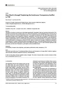
of their long-run average total cost curve in producing hospital bed-days, but stray far from a productively efficient level in terms of producing survival years. While mortality may be the appropriate outcome variable to assess, say, the effectiveness of intensive care units, there is more to efficiency than life expectancy. Individuals seek to maximize utility, and there are costly procedures offering improved health functioning at the cost of increased mortality risk. Other expensive procedures may have no impact on survival rates, but do affect different aspects of health status. For example, surgical treatment for an enlarged prostate improves urinary flow, but it can adversely affect sexual functioning. There is no best treatment for enlarged prostates; some men prefer surgical treatment and others prefer drug treatment or watchful waiting. Thus, allocative efficiency means that the people are treated in the way that they would prefer, generally by being able to choose from the menu of productively efficient procedure^.^ It is important to consider preferences for different types of treatment because it could be the case that people in Miami prefer the more intensive health care services because they prefer such treatment, even if there is no measurable differencein survival. We examine the importance of heterogeneity in preferences in light of the results from recent experiments in informed patient decision making for patients with enlarged prostates and with angina due to coronary artery disease. And while these studies are not specific to Miami, they do suggest that while some preferred the more intensive treatment options, on average patients preferred rates of surgery lower than the level prescribed by most physicians. Thus, the allocative costs of increased levels of surgical intervention could be even larger than those considered in standard cost-benefit trade-off comparisons. 5.2 A Look at Miami and Minneapolis The hospital referral regions for Miami and Minneapolis include a larger area than just the cities themselves. They were determined as part of an effort by the Dartmouth Atlas of Health Care (Wennberg and Cooper 1997) to map the entire United States into 306 regions, each of which has one or more hospitals offering cardiovascular or neurosurgical services. Thus, the Minneapolis hospital referral region (HRR) compriseszip codes whose residents tend to be admitted, or referred to, the major hospitals in Minneapolis, even though the actual region extends well beyond the city limits (see fig. 5.1)? Individuals (and their utilization records) are allocated 4. A more difficult question is whether, at the margin, (productive) medical spending is worth what must be given up in terms of other nonmedical goods. 5. The geographical boundaries of the Miami and Minneapolis areas are defined using methods in the Dartmouth Atlas of Health Care (Wennberg and Cooper 1997). In the atlas, every zip code in the United States was allocated to a hospital service area (HSA); a local
172
Jonathan Skinner and John E. Wennberg
Fig. 5.1 The Miami and Minneapolis HRRs Note: Because hospitals in Miami, and particularly Minneapolis, are magnets for surrounding areas, the actual HRRs for the two cities are quite a bit larger than the actual city boundaries. Note that even if a citizen of Miami, for example, received treatment in Fort Lauderdale, the utilization data is counted in Miami.
to Miami or Minneapolis not because they go to those hospitals, but because they live in zip codes where (typically) the majority of patients do go to such hospitals. These two regions have been shown in prior research to have vastly different patterns of health care spending on a per capita basis. One problem inherent in comparing different regions is that they do in fact differ with regard to community-level disease patterns such as acute myocardial infarction (AMI) and stroke rates. However, even after correcting for such differences, there are still substantial differences in per enrollee rates of utilization (Wennberg and Cooper 1997; Skinner and Fisher 1997). For example, figure 5.2 summarizes data on differences in all per capita Medicare reimbursements, inpatient services, professional and laboratory services, and home health care (Wennberg and Cooper 1997). As the lefthand panel shows, the two cities are clearly at opposite ends of the spectrum in terms of overall Medicare spending. (Each of the fainter dots in hospital (or more than one hospital in the same city or town) that served as a primary source of hospital care. The allocation of zip codes was done on the basis of a 100 percent sample of Medicare hospital discharges. In total, there were 3,436 HSAs in the United States. However, many of these HSAs were small in size, with low-volume local hospitals sending their patients to larger hospitals for complicated procedures. The atlas therefore allocated each of these HSAs to a hospital referral region (HRR); each HRR has at least one hospital that provides major cardiovascular and neurosurgical procedures.
Efficiency and Medicare Spending in the Last Six Months of Life
173
Miami Minneapolis
9,000 2.5
8,000 2.0
P
7.000
3 Y 3
6.000
.-s 0
1.0
3
5.000
0.5
4.000 0.0
3.000
Illness, Price, Age, Sex, 81Race Adjusted 2,000 -
All Services
Inpatient Services
Professional Home &Lab Health Cai Services Services
Illness, Price, Age, Sex, and Race Adjusted Medicare Reimbursements
Ratio of Miami to Minneapolis: 2.12
1.52
3.28
4.14
Fig. 5.2 Medicare reimbursements per enrollee, Miami and Minneapolis Note: The left-hand panel gives the age, sex, race, price, and illness adjusted per person spending by the Medicare program in 1995 for the 306 hospital referral regions studied in the Dartmouth Atlas of Health Care. Spending varies nearly threefold from the lowest to the highest region. Total spending for residents of Miami is 2.1 times greater than Minneapolis on a per person basis. Inpatient reimbursementsare 52 percent higher; those for professional and laboratory services are more than 3.2 times greater; home health spending is more than four times greater.
the diagram represents one of the other 306 hospital referral regions in the United States.) In the right-hand panel, the height of the bars shows the ratio of priceillness-age-sex-race-adjusted levels of services to the United States. In Minneapolis, home health services are 39 percent of the national average, while in Miami they are 60 percent above average, meaning their ratio is roughly 4 to 1. By contrast, the ratio between Miami and Minneapolis for inpatient services is just 1.5 to 1, suggesting that services with the greatest discretionary (and profitability) component-home health and laboratory services-are the ones most sensitive to geographic location. A different way of comparing spending is to look at expenditures and utilization during the last six months of life, a period of time when many Medicare enrollees are quite ill. Comparing spending in the last six months of life is useful for three reasons. First, it is more difficult to invoke plausible clinical scenarios that would explain the observed differences on
174
Jonathan Skinner and John E. Wennberg
the basis of difference in level of illness. Second, this spending has been shown elsewhere to account for a large fraction of total Medicare spending; thus, how people are treated near death has an important impact on the overall Medicare budget (Lubitz and Prihoda 1984). And third, spending levels among this group are probably particularly good markers of how intensely a region’s medical system treats the very sickest, reflecting a sometimes unstated concern that too much is done for people who are going to die anyway. Figure 5.3 shows that the Miami and Minneapolis regions are again at the opposite ends of the national distribution in the intensity of care during the last six months of life. Inpatient Medicare expenditures differ by about 2 to 1 ($14,212 in Miami versus $7,246 in Minneapolis), with an even greater divergence in the average number of ICU days per person in their last six months of life (the right-hand panel). These are indicators of inpatient hospital use. A more telling comparison is the average number of physician visits billed to Medicare for those in their last six months of life. In Miami, the number of primary physician visits is certainly higher, 12.5 visits versus 7.1 visits, or a difference of 76 percent (fig. 5.4). The differences between the two regions, however, are 18,000
5.0
5c
? 4s
4.5
16.000
...... ..... ......... .......... ....
4c
14.000
0
12.000
.:....i i ,
..-
-:e:::z:-
IO,O00
..as
as..
35 30 25
I
............... ............ .............. ............... .......................... ................... .................... .................... ............................. ................... ............... ....... ..... ..... ............ ......
.... .”
4.0
3.5
3.0 2.5 2.0
I .5
8.000
1 .o
6.000
... .. .. ....... ... ....... ...... ......... .......... ........ ....... .............. ........ ............ ................. .................... .............. ................ ............ ............ ................. ....................... .............. ............. .............. ..m.. ......... ..... ... ....
0.5 4,000
.
Percent Admitted toICUDuring the Last 6 Months of Life
0.0
Person During the Last 6 Months of Life
I
Fig. 5.3 Intensity of care in the last six months of life in Miami and Minneapolis Note: Miami is the higher dot; Minneapolis is the lower dot. Among the regions, reimbursements for inpatient care varied more than 2.8-fold, from $5,831 to $16,571. Reimbursements for residents of Miami are about two times greater than Minneapolis (lefi-handpanel). The percentage of enrollees spending one or more days in intensive care varied from a low of about 9 percent to more than 45 percent. Miami is 2.1 times greater than Minneapolis (center panel). The numbers of days spent in intensive care varied more than ninefold. Miami enrollees spent 3.7 times more days in the ICU than Minneapolis enrollees (right-handpanel).
Efficiency and Medicare Spending in the Last Six Months of Life
30.0
w
175
Miami
Q Minneapolis
2
p1
25.0
.-Y 0
20.0
15.0
2
a
E
2
10.0
5.0
0.0
Ratio ofMiami to Minneapolis
Primary Care Physicians
Specialists
I .76
5.40
Fig. 5.4 Average number of primary and specialist visits (per patient) in the last six months of life, Minneapolis and Miami Note: The average number of primary care physician visits is higher in Miami than in Minneapolis (12.5 visits versus 7.1), a difference of 76 percent. The average number of specialist visits is substantially higher in Miami (25.4 risits versus 4.7), a difference of 440 percent. Note that these averages are for the non-HMO population only, and a larger fraction of Miami residents are in HMOs.
most apparent in the average number of specialist visits during the last six months of life: 25.4 in Miami versus 4.7 in Minneapolis, a nearly fivefold difference. Some of this difference could be explained by the greater HMO penetration in Miami, meaning those people who remain in our Medicare claims data (the fee-for-service patients) are sicker. But even if we include the HMO patients in the denominator, thereby assuming they experience no visits to the doctor, the ratio of specialists visits in the region is still about 3 to 1. Thus we believe that the proliferation of specialist visits in Miami is central to the story of why these communities differ so much. It is important to emphasize that the differences in indicators shown above largely reflect a different approach to the treatment of the chronically ill. For some surgical procedures, such as knee replacements and back surgery, rates of surgery are actually lower in Miami.
5.3 How to Interpret Population-Based Differences in Utilization It is important to note that the mere existence of geographicalvariations does not imply the existence of either productive or allocative inefficiency.
176
Jonathan Skinner and John E. Wennberg
One interpretation of variations across areas (theory 1) is they are simply the consequences of underlying differences in illness rates or in patient preferences for treatment. In this view, variations in surgical treatment for enlarged prostates are the consequence in part of mismeasurement; health care researchers are simply misled by geographic variations because they are unable to control for confounding factors. And what variation remains reflects geographical differences in preferences. The second interpretation (theory 2) is that different hospitals and health care systems have very different protocols and standards for conducting surgery and treating illness. In some regions, many more men with enlarged prostates will end up having surgery or many more seriously ill patients will be treated in the ICU than their counterparts-with equivalent preferences and health status-living elsewhere. In this view, “location is destiny,” or in the language of econometrics, location is an instrument. Theory 1 and theory 2 have very different implications. In theory 1, the health care system is productively and allocatively efficient, at least in the sense that all American citizens are receiving treatment consistent with their preferences, and according to a well-established body of scientific evidence and knowledge. Not every hospital will be hugging the productively efficient production “envelope,” of course, because of economies of scale and volume in the treatment of common diseases (e.g., McClellan and Staiger, chap. 3 in this volume). But the important policy issues are not whether the intensity of services in a community such as Miami is much different from that in Minneapolis, but instead whether these regions (together with other regions in the United States) lead to marginal benefits that exceed marginal costs at the national level. Not surprisingly, then, an important policy debate under theory 1 is whether rationing health care on a national level is the appropriate policy to contain potential overproduction in medical technology and services.6 According to theory 2, it is difficult to address national priorities in health care spending if in fact different communities are following such widely different treatment patterns. Instead, the immediate question is, Which community’s rate is right? Theory 2 thus points to exploiting empirically the natural experiments afforded by the geographic variation phenomenon by measuring the correlation between inputs of resources and outputs of health. As we discuss below, the implications of theory 2 are not simply about allocative efficiency (Which rate is right?) but productive efficiency broadly defined (Are some rates always wrong?). In figure 5.5 (upper panel), we consider one way to characterize these differences, where we summarize the intensity of care, Z , on the horizontal 6. For a discussion of global budget caps, see Aaron (1992). A uniform percentage decrease in health care costs will have a much different impact than setting a fixed per capita level of spending across regions.
Efficiency and Medicare Spending in the Last Six Months of Life
177
L (Lifespan)
2,
2
(Intensity)
L (Lifespan)
M
X
(Quality of Life)
Fig. 5.5 A diagrammatic representation of efficiency in health care Note: In the upper panel, the trade-off between the (dollar) intensity of inputs into health care is contrasted with community-level expected lifespan. Point D, for example, corresponds to the maximal level of lifespan given existing medical technology. In the lower panel, a trade-off is shown between lifespan and quality of life.
axis (measured in dollars) and life-year extension on the vertical axis. According to theory 1, most hospitals experience similar intensities of service. Not all health care systems are at the production possibility frontier, but they do not vary significantly in terms of their intensity of care, and any variation that does occur is primarily because of differences in patient health or patient preferences. For example, more people may die in hospital in Miami, but it is because of a lack of family support (or even available nursing home beds) rather than differences in the underlying approach to
178
Jonathan Skinner and John E. Wennberg
treating sick patients.’ According to this theory, we would describe hospitals as clustering around one of the points (perhaps point A), or if differences in preferences lead to differences in intensity of care, along a continuum between points A and B. Thus, it makes sense to talk about national standards of care, because most hospitals are delivering about the same level of intensity. According to theory 2, however, there exist wide variations in how a given disease is treated, leading to much more variable levels of intensity, perhaps ranging from points A to E or beyond, with additional dispersion below the production frontier, as represented perhaps by point C. These exogenous variations, however, can be used to gain information about the nature and shape of the production function. By comparing outcomes between high-intensity and low-intensity areas, one can begin to answer the question of whether the health care system is described best by clusters around point A or at the flat of the curve (point D), where more health spending yields nothing in expected lifespan. Or are some regions on the wrong side of the curve, point E, where the iatrogenic costs of health interventions actually lead to worse outcomes (Fisher et al. 1999)? For hospital procedures devoted simply to helping people to survive, such as ICU facilities, risk-adjusted survival rates are a good measure of outcomes. The analysis becomes more complex once one recognizes the essential multidimensionality of outcomes. For many procedures, the objective is not to maximize lifespan but to improve the overall quality of life. Chemotherapy may have proven benefits in extending survival rates for breast cancer, but it can come at a large cost to the patient. Furthermore, there is tremendous heterogeneity across patients in the trade-off; in one recent study, 12 percent of the sample would undergo standard chemotherapy for metastatic breast cancer in return for an expected additional lifespan of just one week. By contrast, 28 percent of the sample would not undergo standard chemotherapy in return for increased longevity of 18 months (McQuellon et al. 1995). Similarly, there is wide variation in preferences for chemotherapy to treat advanced-stage non-small cell lung cancer (Brundage, Davidson, and Mackillop 1997; Silvestri, Pritchard, and Welch 1998; McNeil et al. 1982). For example, in the Silvestri, Pritchard, and Welch study, all respondents had been treated with chemotherapy previously for advanced non-small cell lung cancer. The authors write about the patients’ response to a hypothetical case involving the decision of whether to elect chemotherapy: “In the setting of severe toxicity, for example, 5 (6%) patients would choose chemotherapy for only 1 week of additional survival while 9 (1 1%) others would not choose the therapy even when offered 24 months of additional survival. In both scenarios, however, less than half the patients would choose chemotherapy given the 7. Although Miami does not lack for home health care services on a per capita basis.
Efficiency and Medicare Spending in the Last Six Months of Life
179
‘best guess’ of the actual average benefit-a 3 month difference in median survival.” This heterogeneity in preferences makes it very hard to calculate a single “quality-adjusted life year” (QALY). For the average person, the loss in functioning and pain is not worth the extra life years; thus, the QALY associated with chemotherapy would probably be negative. But clearly, the average QALY is relevant only for the average person. For some people, the QALY associated with chemotherapy is positive; for others, clearly negative. Thus the upper panel of figure 5.5 is not an adequate representation of the types of trade-offs facing individual patients. The lower panel in figure 5.5 demonstrates the problem of treatment choice when preferences are heterogeneous. For simplicity, we consider just the trade-off between lifespan and a generic quality of life measure X , shown on the horizontal axis. Thus we are implicitly considering a threegood utility function that depends on nonmedical consumption Y - 2, where Y is income and 2 (as before) is health care resources, lifespan L, and quality of life X . Medical technology provides a trade-off between X and L; the opportunity set MM’ is shown for a given level of Z equal to Z , . This represents the possible trade-offs between lifespan and quality of life given the current state of medical technology. (A similar trade-off curve exists for lower or higher levels of Z , one hopes that more 2 yields a trade-off curve to the northeast of MM’.) In this case, the point C, which appears to be productively inefficient in the upper panel, is actually preferred by some patients, shown by the (Y preference ordering, while point B is preferred by a different group of patients with preference orderings p. This is why we cannot simply “quality adjust” those life years; the different groups (Y and p disagree over the relative weights placed on lifespan extension versus quality of life. The problem becomes more complicated once one accounts for a third class of medical procedures that are unlikely to have much impact on life expectancy but that will have a larger effect on different aspects of the quality of life. For example, it is unlikely that surgical treatment for an enlarged prostate will have a large impact on expected lifespan, but it might be expected to affect symptoms (positively) and sexual functioning or incontinence (adversely). Thus, the decision to choose surgical treatment of enlarged prostates is taken along the flat of the survival curve (point D), where increased spending will yield no benefit in terms of lifespan but will affect different dimensions of one’s quality of life, X . There are two points here. The first is that “best practice” medical care does not guarantee allocative efficiency. There is often a wide range of treatments available for a given problem, and which treatment is chosen should depend on the preferences of the individual patient (i.e., whether he or she is an [Y or p type). If an [Y type receives treatment option B (perhaps because the alternative, C , was not offered or was downplayed by the physician), then allocative inefficiency would result. And second,
180
Jonathan Skinner and John E. Wennberg
it seems unlikely that preferences among the various choices could vary systematically across regions in a way to generate such large differences in treatment patterns, particularly if the regions are (on average) in the vicinity of point D. Of course, without further research on actual preferences in the two regions, we cannot prove that preferences do not differ to the degree suggested by treatment variation, but the evidence (discussed below) suggests that, if anything, individuals prefer the less-intensive options when given the choice.8
5.4 Do Health Differences Explain Variation in End-of-Life Expenditures? We return to asking whether theory 1 might explain the dramatic differences in health care spending in the last six months of life. This question is best seen as part of the very large and sometimes contentious debate over “small area variations.” It is well established that differences in per capita medical utilization across the United States and other countries exists. Typically, researchers include as many “supply-” and “demand-” related measures as can be mustered, but there is still a large residual that remains. The battle is over the residual: Does it represent exogenous differences in practice patterns (theory 2), or does it represent preference or health-related factors that are simply not measured by the researcher (theory l)? Without delving into details, we simply note that most research is unable to explain the variations using conventional measures of health needs (e.g., Wennberg and Fowler 1977; Henke and Epstein 1991; Wennberg and Cooper 1997; Fisher et al. 1994; Wennberg et al. 1989; Gruber and Owings 1996; Skinner and Fisher 1997; although see Green and Becker 1994).9Thus, under theory 1, regional variation is explained more by tastes (or unmeasured health needs), perhaps reflected in the decision of individuals to initiate contact with physicians (e.g., Escarce 1993; Folland and Stano 1989). The issue of whether to initiate contact with physicians, however, is not likely to be as important among this sample of Medicare enrollees in the last six months of life. Instead, ‘the observed differences most likely reflect the intensity of care. Still, it may be the case that the intensity of medical spending in the last 8. A final issue is whether people choosing between more- and less-intensive treatment on the basis of quality of life, as in the prostate example above, should face copayments for the more-intensive treatment. If, in fact, survival rates are not affected by the decision to treat enlarged prostates surgically, then might not patients be required to face some fraction of the extra resource cost? 9. There is also a literature suggesting that small area variations can be explained simply by random variation in averages of regions with small sample sizes (Diehr et al. 1990). However, the research using often 100 percent samples of Medicare data (e.g., Wennberg and Cooper 1997) shows that the regional variation is not due to small sample problems.
Efficiency a nd Medicare Spending in the Last Six Months of Life
Regression Explaining Medicare Part A Reimbursements in the Last Six Months of Life, by Hospital Referral Region
Table 5.1
~
~
181
Regression Excluding Health Resource Variables
Regression Including Health Resource Variables
Coefficient
Coefficient
t-Statistic
t-Statistic
~~
AM1 Stroke (CVA) GI bleeding Lung cancer Hip fractures Hospital beds Specialist MD Primary MD Family practice MD Constant
-170.8 53.9 770.2 1,185.4 -514.1
2.9 0.6 5.1 4.1 3.8
4,505.6
3.2
-93.0 83.4 341.9 -23.9 -343.9 1,146.2 38.4 -8.0 14.26 1,609.5
2.0 1.2 2.8 0.1 3.1 8.8 7.2 0.7 3.5 1.4
Note: The dependent variable is the price-adjusted average Medicare reimbursements per person in their last six months of life. In the first regression, R2= 0.18; in the second RZ = 0.54. Each observation corresponds to a hospital referral region (HRR), of which there are 306. All regressions are weighted by the number of Medicare enrollees in the HRR. All of these variables (except the percent not-for-profit) have been adjusted for age, sex, and race differences; thus, we do not include these variables into the regression.
six months of life is the consequence of patients in some regions dying of diseases requiring more costly palliative care. Thus, we would like to test the hypothesis of whether end-of-life expenditures are related to the mix of diseases in the hospital referral region (HRR). To do this, we regress the HRR-level measures of average inpatient spending in the last six months of life as a function of Medicare hospital admissions in 1994-95 for a set of common diseases that are reasonable measures of underlying community health levels: AMI, stroke, gastrointestinal (GI) bleeding, hip fractures, and lung and colon cancer (see Wennberg and Cooper 1997 for details). All regressions were weighted by the Medicare population in each of the 306 HRRs. Table 5.1 displays coefficients from this first regression correlating just health indicators with spending near the end of life. There are generally significant effects, and the adjusted R2is 0.18. The coefficient on AMI, for example, is negative; this suggests that people with AM1 are more likely to die quicker, and at lower cost, than people with other diseases such as lung or colon cancer.'O While these diseases account for a large fraction of overall mortality, they explain only a small fraction of the variance in spending near the end of life. 10. We have included both types of cancer in one category because of relatively small sample sizes, particularly in later regressions.
182
Jonathan Skinner and John E. Wennberg
A more general regression model is also presented in table 5.1 that includes resource levels: hospital beds per thousand, specialist MDs per 100,000, primary care MDs per 100,000, and family practitioners per 100,000. The adjusted R2 rises to 0.54, and the age-sex-race-adjusted bed capacity is highly significant. The impact of primary care physicians on Medicare end-of-life spending is not significant (and is, in fact, negative), although the effect of family practitioners-holding constant the number of overall primary care physicians-is positive with a modest coefficient. However, the impact of specialists is of the greatest magnitude and significance. One could argue, of course, that in the long term, the supply of physicians in Miami and Minneapolis is not random; perhaps physicians (or specialists) are attracted to Miami because of the heavy volume of practice. The point remains that the characteristics of the regions that should matter most under theory 1 for end-of-life spending-disease burdens-explain less than 7 percent of the overall difference between Miami ($14,212) and Minneapolis ($7,246). In sum, we find it plausible to adopt, as a working hypothesis, that Medicare spending in the last six months of life contains a strong degree of exogeneity across regions.lI 5.5 Does the Higher Spending Lead to Better Outcomes? Even if there are real differences in how people get treated among areas, it still may be the case that people in regions with high levels of health care do better; thus, the extra expenditures in Miami could be justified by the improved health status of its population.12 We address this question in two ways, both using data from the entire United States. First, we consider whether differences in end-of-life spending have an impact on the overall age-sex-race-adjusted mortality rates in the United States. Using the statistical methods developed in Fisher et al. (1999), we perform a logistic regression on life expectancy for a 20 percent sample of the Medicare population (more than 5 million individuals),controlling for a wide battery of possible confounding factors such as levels of disability, poverty rates, and underlying levels of the five types of diseases noted above. Table 5.2 provides estimates of the coefficient of interest-the partial impact of spending in the last six months of life on mor11. Given that these two cities were chosen on the basis of their extreme differences in treatment patterns, it might be expected that they would exhibit the greatest deviation from the norm. The point holds, however, for other regions also. Note also that our claim to exogeneity with respect to spending patterns on patients near death does not require that one accept a “supplier-induced demand” view of the health care system, only that variations in medical spending on patients near death is not simply the consequence of health differences. 12. Thus our approach is similar to those comparing intensity of care and outcomes in New Haven and Boston; see Fisher et al. (1994) and Wennberg et al. (1989).
Efficiency a n d Medicare Spending in the Last Six Months of Life Table 5.2
183
Logistic Regression of Mortality in the Medicare Population
Variable Spending in last 6 months ICU days in last 6 months
Odds Ratio
95% Lower Boundary
95% Upper Boundary
Significance
1.001 1.008
0.999 1.003
1.003 1.014
0.408 0.002
Note: In the table above, the dependent variable is whether the individual lived or died in the benchmark year of 1990. The logistics odds ratio is shown for price-adjusted expenditures in the last six months of life, or for the average number of days spent in an ICU in the last six months of life. These variables (for 1994-95) are calculated for each hospital service area, of which there are 3,436 in the United States. Thus, the level of analysis is at a finer level of geography than for the standard hospital referral region used in most of the other statistical analyses. There are more than 5 million observations in the regression. This regression is adopted from Fisher et al. (1999). Covariates include age-sex-race-specificcells, and from the census: median family income (for blacks and whites separately) in the population over 65, percent of population 65+ below the poverty level, education (less than grade 12, high school graduates, and college graduates), percent in rural areas, percent in urbanized areas, percent with work disabilities, self-care limitations, and mobility limitations (all 65 +).
tality-along with a description of the additional variables; also see the appendix for a full set of regression results. Briefly, there appears to be little correlation between the intensity of care near the end of life and mortality rates, whether intensity is measured by spending, days in the hospital, or ICU days near the end of life. If anything, there is a slight positive (and highly significant) correlation between ICU days and mortality rates; an increase of 1.0 in the average number of ICU days in the last six months of life is predicted to increase mortality rates by 0.8 percent. One objection to this analysis is that there may be reverse causation; sicker regions would tend to have higher spending near the end of life, and hence generate a spurious correlation between the two variables (possibly masking the true negative correlation). This objection, however, carries less weight given that we are restricting our measure of spending to the universe of people near death. Sicker communities might well spend more per Medicare enrollee and experience a higher mortality rate, but it is not clear that sicker communities would spend more per person for the set of people who die. Still, it is useful to consider this question using a different approach that focuses on disease-specific mortality rates. We selected a 5 percent sample of Medicare enrollees who were diagnosed with diseases that almost surely caused admission to the hospitalAMI, stroke, GI bleeding, hip fractures, and lunglcolon cancer-for the two-year period 1992-93. Conditional on having an AM1 or stroke, one might expect that the underlying health status, and survival probabilities should be similar across areas, thus potentially correcting for the reverse causality problem. As our marker for the intensity of health care in the
184
Jonathan Skinner and John E. Wennberg
Table 5.3
Logistic Regressions of Mortality in the Medicare Population for Five Specific Health Conditions
Mortality Variable 6-month (full sample) 6-month (full sample? 90-day (full sample) 6-month (AMI) 6-month (stroke) 6-month (hip fracture) 6-month (GI bleed) 6-month (cancer)
Odds Ratio
95% Lower Boundary
95% Upper Boundary
Significance ( p Value)
0.998 1.015 0.994 0.989 0.994 1.019 1.003 0.997
0.986 0.986 0.981 0.968 0.974 0.991 0.972 0.949
1.010 1.045 1.007 1.011 1.015 1.048 1.034 1.047
0.762 0.321 0.348 0.333 0.566 0.187 0.173 0.892
Note: The dependent variable is whether the individual lived or died within the 6-month (or 90-day) period, conditional on having been admitted to hospital for one of the five initiating conditions during the years 1992-93. The logistics odds ratio is shown for price-adjusted expenditures in the last six months of life (in units of $1,000) by HRR or (as in row 2) the average number of ICU days by HRR, again in the last six months of life. The overall sample size is 53,564. Average 6-month mortality rates are 22.6 percent; average 90-day rates are 18.7 percent. 'This logistics odds ratio is shown for the average number of ICU days in the last six months, by HRR.
region (or HRR), we also include the average Medicare spending and average number of ICU days for each HRR during the last six months of life (for all residents in 1994-95).13 We also include as independent variables controls for age, sex, and race; details of the logistic analysis are reported in table 5.3, with the full results from one regression shown in the appendix. Once again, there does not appear to be any positive impact on mortality of the region-level intensity of care for enrollees in the last six months of life (either measured in dollar terms or in ICU days). One might object to this analysis because end-of-life spending is probably accounted for largely by treatment for chronic diseases, not for sudden medical emergencies such as AM1 and stroke; thus, our indicator may not summarize well how a given AM1 or stroke would be treated. Another way to approach this problem is to calculate the diseuse-specific levels of health care spending by HRR. We do this by first regressing Medicare reimbursements, at the individual level, on age, sex, race, and illness dummy variables. This regression reflects possible differences in Medicare spending as the consequence of demographic or illness variation across regions. We then average the residuals in each region (after controlling for these demographic and illness factors); these HRR-level constructed 13. While these data are from the period 1992-93 and the end of life data are from the period 1994-95, the temporal mismatch is not likely to bias our results substantially, given the secular stability in spending patterns of HRRs.
Efficiency and Medicare Spending in the Last Six Months of Life
185
residuals were highly correlated with HRR-level spending in the last six months of life.I4We then used the HRR-level residuals in a second-stage regression seeking to explain mortality rates, with insignificant results (regressions not reported). We regard these results as preliminary, however, given the larger sample sizes necessary for statistical power. Of course, it could be that our measure of outcome, survival, does not adequately reflect the true underlying quality of life enjoyed by patients in Miami over those in Minneapolis. While we have no direct evidence on quality-of-life outcomes in the two regions, we can turn to more general evidence from research on whether patients in fact prefer these more intensive forms of treatment. 5.6 Do Patients Prefer More Intensive Levels of Health Care? The Case of Surgery In this section, we return to the issue of preferences in health care and to the notion that specific surgical procedures could improve the quality of life even if survival rates are not improved (or worsened). Thus, we seek to address whether, in fact, patients prefer the more intensive patterns of health care. In contrast to treatment intensity during the last six months of life, the goal of surgery is often to increase the quality of life, not the length of life. In fact, the risks inherent in surgery often mean that improvements in the quality of life come at the cost of a small increase in the chance of early death. But length of life versus quality of life is not the only trade-off. For example, most patients who undergo surgery for an enlarged prostate gland experience a change in sexual function (retrograde ejaculation), and there is a risk of incontinence and impotence. Men with enlarged prostates thus face a dilemma: Although surgery provides the best option for reducing symptoms, it involves trade-offs with tangible risks. Men and women with stable angina benefit more in terms of immediate reduction in symptoms by undergoing coronary artery revascularization. But again, there are trade-offs. For example, among the Medicare population, mortality from bypass surgery is about 2 percent; a substantial number of those who undergo this operation experience a loss in short-term memory and other impairments of cognition. Research shows that men, when fully informed about the options and their possible consequences, differ substantially in their preferences for surgery. For the case of enlarged prostates, the objective of the surgery is to improve the symptoms, including difficulty or strain in urination. In one study, a sample of men with prostate symptoms was presented with 14. In other words, there is a strong HRR-level correlation between the intensity of spending in the last six months of life and the intensity of spending more generally for these common acute conditions.
186
Jonathan Skinner and John E. Wennberg
Table 5.4
Factors Predicting Choice of Surgery for Enlarged Prostate Gland Variable Symptom score Mild Moderate Severe Rating of symptoms Positive/mixed Negative Rating of impotence Positivdmixed Negative
~~~~~
Odds Ratio
95% Confidence Interval
0.09
0.01, 0.72
1.48
0.6, 3.6
7.0
2.9, 16.6
0.20
0.08, 0.48
~~
Source; Barry et al. (1995). Note; N = 347; 32 of these men underwent a prostatectomy. The table presents the results of a logistic regression model to predict choice of surgery. Symptoms are whether the patient experiences difficulty with urinating. Although in the univariate model patients with severe symptoms were 2.4 times more likely to choose surgery than those who were moderately symptomatic, only 21 percent of those with severe symptoms actually choose surgery. In the multivariate model, the odds ratio dropped to 1.48 and was no longer significant. By contrast, the ratings patients gave to their symptoms ( i c , how much they were bothered by them) and concern about impotence were strong predictors of choice.
information about the risks and benefits of surgery, and then asked about their own preferences (Barry et al. 1995); a summary of results from a logistic regression is shown in table 5.4. The partial effect of severe (rather than moderate) symptoms is to raise the chance of choosing surgery (odds ratio of 1.48, or an increase of 48 percent), but the results are not significant.I5 By contrast, two much better (and significant) predictors of whether the patient chooses surgery were (1) if the given symptoms bothered the patient (odds ratio of 7.0) and (2) the degree of concern about the chance of impotence (odds ratio of 0.2). In other words, the most important predictors of whether the men chose surgery was less the severity of the symptoms, and more the degree to which the symptoms bothered the patient and their concerns about the possibility of impotence. Thus, geographical regions have the potential for significant allocative inefficiency, even if their average rates are “right.” The necessary condition for efficiency is that the patients desiring surgery are the ones that get it and the patients who don’t want surgery don’t get it. Two experiments designed to study the effects of shared decision making on the rates of surgery provide an insight into the extent that surgery may be misallocated in the United States. The first, conducted in two staff model HMOs, implemented a change in the way clinical decisions were 15. A mild symptom score reduced (significantly) the odds of having surgery. However, mildly symptomatic men generally do worse after surgery and probably should not be offered the option.
Efficiency and Medicare Spending in the Last Six Months of Life
187
made for prostate surgery. After viewing an interactive video that informed patients about the risks and benefits of alternative treatment, patients were encouraged to choose the treatment they would prefer. Surgery rates were measured before and after the video was introduced, and also with reference to a control population. In each HMO, rates dropped about 40 percent, suggesting that the amount of surgery formally “prescribed” by the HMO exceeded the amount that informed patients wanted (Wagner et al. 1995). The resulting demand for prostate surgery is shown in figure 5.6; interestingly, this benchmark was less than virtually every region in the United States. Similarly, a randomized trial of a shared decision making program for treatment of coronary artery disease suggests that patient demand for revascularization (at least in Canada) may be lower than the rate of revascularization in nearly every HRR in the United States; see figure 5.6 (Morgan et al. 1997). These findings suggest a point that should be easily absorbed by econo-
... .... ..... ...... ........ .. .......... ........... ............ ...................... ..................... .............. ......................... .............................. ........................... ................... .......................... ................ ............. .............. .... ... ...
...... .. ..... .... ....... .... ....... ......... .................... ........ .................................. ...................................... ............................ .................... ........ ................... ............. ...... ...
..
7 I
Fig. 5.6 Actual and desired rates of surgery for enlarged prostate and angina Source: Wagner et al. (1995); Morgan et al. (1997). Note: The distribution of rates in the left-hand panel is for surgery for enlarged prostate gland (benign prostatic hyperplasia [BPH]) among Medicare enrollees living in the nation’s 306 hospital referral regions. The distribution in the right-hand panel is for coronary artery revascularization. A study of the effects of involving patients directly in their choice of surgery was conducted among patients with enlarged prostates in two staff model HMOs and among patients with angina in Toronto, Canada. In the prostate study, when patients were fully informed about the risk and benefits of alternative treatments and encouraged to participate actively in the choice of treatment, the population-based rate of surgery dropped 40 percent compared to controls. In the Ontario study, the rate dropped about 24 percent, even though the baseline rate in Ontario was substantially less than any rate observed in the United States.
188
Jonathan Skinner and John E. Wennberg
mists. If patients are both less enthusiastic about surgery than the national averages would suggest, and show heterogeneity in their underlying preferences toward outcomes from surgery, there is a potential Pareto improvement by allowing them to make their own choice, even if the choice is ultimately to defer to the physician’s choice. In the cases considered above, society gains: Patient welfare is improved, and expenditures on health care are reduced.
5.7 Discussion and Conclusion Regions across the United States appear to have adopted much different strategies for treating Medicare patients. In this paper, we compare expenditures and ICU utilization across these hospital referral regions for elderly people in their last six months. We choose people in the last six months of life because they are all quite sick, and thus we can partially control for geographical differences in the underlying levels of disease. Medicare expenditures in the last six months of life are twice as high in Miami as in Minneapolis, and the average number of specialist visits is nearly five times higher. We have argued that these differences are unlikely to be explained simply on the basis of differences in health status or even preferences. In sum, we find little support for our theory 1 (that variation in health care treatment simply reflects differences in preferences or in underlying health status) and much more support for the notion that the variation in health status is to some extent exogenous (theory 2). Variation in Medicare spending alone does not necessarily imply inefficiency in the distribution of health care. After all, sick people in regions with more intensive treatment patterns may survive longer, thus (possibly) justifying the extra expenses. However, using two much larger samples of individuals-one a 20 percent sample of all Medicare enrollees and the other a 5 percent sample of Medicare patients hospitalized with AMI, stroke, GI bleeding, and cancer-we find no evidence that higher levels of spending translate into extended survival. But it may still be the case that people in the high-intensity areas prefer the more intensive treatment. And while we do not know conclusively that people in such regions would prefer more intensive health care, we do know that patients living in other areas, if provided with information to make their own choices, generally prefer less, not more, intensive health care. Thus, we conjecture that on the basis of economic efficiency, Miami may fall short of Minneapolis. Our results may appear inconsistent with recent evidence documenting the striking secular gains in survival rates following heart attacks (e.g., Cutler et al. 1996).16However, our test for the effectiveness of health care relates solely to regional differences in the intensity of care in a given year, and hence for a given body of medical knowledge. 16. We are grateful to Frank Lichtenberg for pointing this out to us.
Efficiency and Medicare Spending in the Last Six Months of Life
189
One question we are not yet able to answer is, Why do physicians and hospitals in Miami adopt such an intensive strategy for health care, and in Minneapolis, a much less intensive approach? One reason could be the sheer amount of resources in Miami: more hospital beds per thousand (3.2 versus 2.6) and more specialists (146 per 100,000 versus 100).17Another explanation could be the much higher ratio of for-profit hospital beds in Miami: 56 percent versus less than 2 percent in Minneapolis. But there is still a substantial residual left unexplained even after accounting for supply factors. And even these “causal” factors are suspect, since for-profit hospital chains or physicians may be most likely to locate where practice styles are most aggressive.I8 Perhaps the for-profit hospitals in Miami exerted a larger impact on the not-for-profits because of more dense markets in Miami causing the notfor-profits to imitate the behavior of the for-profits, in the sense of Cutler and Horwitz (chap. 2 in this volume). Alternatively, the key to explaining why Miami is so different could be in the structure of physician groups rather than the h0spita1s.l~The interaction between patient demand and physician behavior is also important in understanding the practice of medicine in Miami; perhaps elderly patients come to expect numerous referrals as the norm, and would suspect physicians who do not refer them to other physicians. The differences in practice patterns between these two cities (and across the United States more generally) appear to be real, but they are somewhat resistant to an entirely economic structural explanation. Ultimately, some part of the story may be the (random) emergence of small groups of entrepreneurial physicians who set the practice style for the entire area. A recent Wall Street Journal article, for example, identified a single aggressive cardiology physicians group as the reason for why Lubbock, Texas, had one of the highest per capita rates of angioplasty in the country (Anders 1996).20 Whether regional differences in Medicare utilization can ultimately be explained in a structural model of medical practice, or whether these regional differences are the outcome of a “path-dependent” process originating with a few entrepreneurial physicians, is a topic for future research. 17. There are also more primary care physicians in Miami (83 versus 68 per lOO,OOO), although as noted above, primary care physicians are not correlated with Medicare spending in the last six months of life. 18. Even if physician supply, for example, is increased in Miami because of the more intensive practice style, we can still view the resulting treatment intensity as exogenous from the point of view of a production function. 19. One conference participant suggested that fraud could also play a part in the high number of physician visits in Miami. Ironically, were the difference attributed to fraud, the efficiency considerations would be much more benign. Fraud is simply transfers from the government to physicians without any real resource cost except the effort of signing forms and filing them. There i s a real resource cost, the alternative activities of the physician, if the doctor is actually visiting the patient. 20. The group expanded by advertising in the New England Journal of Medicine for cardiologists seeking potential incomes in excess of $1 million.
Appendix Table 5A.l
Logit Regression Explaining Mortality (from AU Causes) in the Medicare Population Coefficient (95% Confidence Interval)
Medicare spending in the last 6 months of life ($ thousands per capita) AMI/100 CVA (stroke)/100 Hip fracturellO0 Colon cancer/100 Lung cancer/100 Percent with income $15,000-$20,000 Percent with income > $20,000 Percent in poverty Percent moved Percent rural Percent in city
.0015
Coefficient (95% Confidence Interval) Percent in nursing home
(-,001, ,004)
,0347 (.021, .048) ,0345 (.021, .048) ,0296 (.012, ,047) -.0128 (-,043, ,018) -.0364 (- .098, ,026) - .0240 (-,035, -.012) -.0265 (-,042, -.011) - .0041 (-,011, ,003) -.0010 (- .006, ,004) -.002 (- .004, - .OOO) ,0052 (.004, ,007)
Percent Hispanic Percent single Percent high school dropout Percent high school graduate Medicare HMO percentage Percent employed (> age 16) Percent with working disability Percent with self-care limitation Percent with mobility limitation Per capita MDs 150-200 per 100,000 Per capita MDs > 150-200 per 100,000
,0540 (.048, .060) -.0126 (-,017, -.008) .0218 (.0159, ,0277) .0440 (.037, ,051) ,0386 (.033, ,044) ,0016 (.001, .002) ,0531 (.048,.059) ,0352 (.027, .044) - .OO83 (- .022, ,005) ,0213 (.007, .035) .O123 (.001, ,023) ,004
(-,009, ,017)
Note: The reported coefficients are for the logit regression index and are not odds ratios. These results control for age-sex-race dummy variables (it., a dummy variable for a nonblack female age 70-74) and regional dummy variables (coefficients not reported). The number of age-sex-race-zip-code cells is 311.146.
Table 5A.2
Logit Regression Explaining Mortality for a Cohort in the Medicare Population with Specific Diseases Coefficient (95% Confidence Interval)
Coefficient (95% Confidence Interval) Medicare spending in the last 6 months of life ($ thousands per capita) AMI/l,OOO CVA (stroke)/1,000
GI bleedindl ,000 Lung and colon cancerl1,OOO For-profit ratio Male age 65-69 Male age 70-74
.0998 (0.986, 1.010) 2.474 (2.314, 2.645) 2.323 (2.179, 2.476) 1.077 (0.999, 1.161) 1.014 (0.914, 1.125) 1.094 (0.984, 1.217) 0.964 (0.852, 1.092) 1.311 (1.167, 1.474)
Male age 75-79 Male age 80-84 Male age 85-90 Male age 90+ Female age 70-74 Female age 75-79 Female age 80-84 Female age 85-89 Female age 90+
1.802 (1.608, 2.021) 2.475 (2.204, 2.778) 3.533 (3.106, 4.019) 6.039 (5.168, 7.056) 1.176 (1.044, 1.324) 1.483 (1.325, 1.659) 1.922 (1.723, 2.144) 2.576 (2.305, 2.879) 3.829 (3.407, 4.302)
192
Jonathan Skinner and John E. Wennberg
References Aaron, Henry J. 1992. Health Care Financing. In Setting Domestic Priorities: What Can Government Do? ed. Henry J. Aaron and Charles L. Schultze. Washington, D.C.: The Brookings Institution. Anders, George. 1996. In Lubbock, Texas, a Weak Heart Gets the Full Treatment. The Wall Street Journal, 16 July, A l , A5. Barry, Michael J., Floyd J. Fowler, Jr., Albert G. Mulley, Jr., Joseph V. Henderson, Jr., and John E. Wennberg. 1995. Patient Reaction to a Program Designed to Facilitate Patient Participation in Treatment Decisions for Benign Prostatic Hyperplasia. Medical Care 33 (8): 771-82. Breyer, F. 1987. The Specification of a Hospital Cost Function: A Comment on the Recent Literature. Journal of Health Economics 6: 147-58. Brundage, M. D., J. R. Davidson, and W. J. Mackillop. 1997. Trading Treatment Toxicity for Survival in Locally Advanced Non-Small Cell Lung Cancer. Journal of Clinical Oncology 15:330-40. Cutler, David M., Mark McClellan, Joseph P. Newhouse, and Dahlia Remler. 1996. Are Medical Prices Declining? NBER Working Paper no. 5750. Cambridge, Mass.: National Bureau of Economic Research. Diehr, P., K. Cain, F. Connell, and E. Volinn. 1990. What Is Too Much Variation? The Null Hypothesis in Small Area Variation. Health Services Research 24: 741-71. Escarce, Jose J. 1993. Would Eliminating Differences in Physician Practice Style Reduce Geographic Variations in Cataract Surgery Rates? Medical Care 3 1: 1106-18. Fisher, Elliott S., John E. Wennberg, Therese A. Stukel, and Sandra M. Sharp. 1994. Hospital Readmission Rates for Cohorts of Medicare Beneficiaries in Boston and New Haven. New England Journal of Medicine 331:989-95. Fisher, Elliott, John E. Wennberg, Therese A. Stukel, Jonathan Skinner, Sandra M. Sharp, Jean L. Freeman, and Alan M. Gittelsohn. 1999. Associations among Hospital Capacity, Utilization, and Mortality of U.S. Medicare Benificiaries. United States: Might More Be Worse? Health Services Research. Forthcoming. Folland, S., and M. Stano. 1989. Sources of Small Area Variation in the Use of Medical Care. Journal of Health Economics 8:85-107. Friedman, B. and M. V. Pauly. 1981. Cost Functions for a Service Firm with Variable Quality and Stochastic Demand: The Case of Hospitals. Review of Economics and Statistics 63:610-24. Gaynor, M., and G. F. Anderson. 1995. Uncertain Demand, the Structure of Hospital Costs, and the Cost of Empty Hospital Beds. Journal of Health Economics 14 (3): 291-318. Gold, Marthe R., Louise B. Russell, Joanna E. Siege], and Milton C. Weinstein, eds. 1996. Cost-Effectiveness in Health and Medicine. New York: Oxford University Press. Green, Lee A,, and Mark P. Becker. 1994. Physician Decision Making and Variation in Hospital Admission Rates for Suspected Acute Cardiac Ischemia: A Tale of Two Cities. Medical Care 32 (1 1): 1086-97. Gruber, Jonathan, and Maria Owings. 1996. Physician Financial Incentives and Cesarean Section Delivery. Rand Journal of Economics 27 (1): 99-123. Henke, Curtis J., and Wallace V. Epstein. 1991. Practice Variation in Rheumatologists’ Encounters with Their Patients Who Have Rheumatoid Arthritis. Medical Care 29 (8): 799-812.
Efficiency and Medicare Spending in the Last Six Months of Life
193
Lubitz, James, and Ronald Prihoda. 1984. The Use and Costs of Medicare Expenditures in the Last 2 Years of Life. Health Care Financing Review 5 (3): 117-31. McEachern, William A. 1994. Economics: A Contemporary Introduction. Cincinnati, Ohio: South-Western Publishing Co. McNeil, Barbara, Stephen G. Pauker, Harold S. Sox, Jr., and Amos Tversky. 1982. On the Elicitation of Preferences for Alternative Therapies. New England Journal of Medicine 306 (21): 1259-62. McQuellon, Richard I?, Hyman B. Muss, Sara L. Hoffman, Greg Russell, Brenda Craven, and Suzanne B. Yellen. 1995. Patient Preferences for Treatment of Metastatic Breast Cancer: A Study of Women with Early-Stage Breast Cancer. Journal of Clinical Oncology 13 (4): 858-68. Morgan, M. W., R. B. Deber, H. A. Llewellyn-Thomas, P. Gladstone, R. J. Cusimano, K. O’Rourke, and A. S. Detsky. 1997. A Randomized Trial of the Ischemic Heart Disease Shared Decision Making Program: An Evaluation of a Decision Aid. Journal of General Internal Medicine 12, no. 1 (April supp.): 62. Rosko, Michael D., and Robert W. Broyles. 1988. The Economics of Health Care: A Reference Handbook. New York: Greenwood Press. Silvestri, Gerard, Robert Pritchard, and H. Gilbert Welch. 1998. Preferences for Chemotherapy in Patients with Advanced Non-Small Cell Lung Cancer: Descriptive Study Based on Scripted Interviews. British Medical Journal 3 17 (7161): 771-75. Skinner, Jonathan, and Elliott Fisher. 1997. Regional Disparities in Medicare Expenditures: An Opportunity for Reform. National Tax Journal 50 (3): 413-25. Wagner, E. H., P. Barrett, M. J. Barry, W. Barlow, and F. J. Fowler. 1995. A Randomized Trial of a Multimedia Shared Decision-Making Program for Men Facing a Treatment Decision for Benign Prostatic Hyper&& Medical Care 33: 765-70. Wennberg, John E., and Megan M. Cooper, eds. 1997. The Dartmouth Atlas of Health Care 1998. Chicago: American Hospital Publishing. Wennberg, John E., and Floyd J. Fowler, Jr. 1977. A Test of Consumer Contribution to Small Area Variations in Health Care Delivery. Journal of the Maine Medical Association 68 (8): 275-79. Wennberg, John E., J. L. Freeman, R. M. Shelton, and T. A. Bubolz. 1989. Hospital Use and Mortality among Medicare Beneficiaries in Boston and New Haven. New England Journal of Medicine 321 (17): 1168-73.
This Page Intentionally Left Blank