How robust is quicksort average complexity? Suman Kumar Sourabha
Soubhik Chakrabortyb*
a
b
University Department of Statistics And Computer Applications T. M. Bhagalpur University Bhagalpur - 812007 India
Department of Applied Mathematics B. I. T. Mesra Ranchi-835215 India
Abstract The paper questions the robustness of average case time complexity of the fast and popular quicksort algorithm. Among the six standard probability distributions examined in the paper, only continuous uniform, exponential and standard normal are supporting it whereas the others
are supporting the worst case complexity measure. To the
question -why are we getting the worst case complexity measure each time the average case measure is discredited? -- one logical answer is average case complexity under the universal distribution equals worst case complexity. This answer, which is hard to challenge, however
gives
no
idea
as
to
which
of
the
standard
probability
distributions come under the umbrella of universality. The morale is that
average
case
complexity
measures,
in
cases
where
they
are
different from those in worst case, should be deemed as robust provided
only
probability
they
get
the
distributions,
support both
from
at
least
discrete
and
the
standard
continuous.
Regretfully, this is not the case with quicksort.
Keywords Quicksort Algorithm; average complexity; robustness *Corresponding author. Email addresses:
[email protected] (S. Chakraborty)
[email protected] (S. K. Sourabh)
AMS 2000 classification code: primary: 11Y16; secondary: 68Q25.
1
1. Introduction: It has been clearly stated in several papers ([1]-[4]) and reviews (see e.g. [5]) that (i)
time is an operation weight and not an operation count [1] [2]
(ii)
a statistical complexity bound weighs rather than counts the operations unlike a mathematical bound. Also, whereas a mathematical bound is operation specific, a statistical bound takes all operations collectively [3]. A table of differences between math bounds and stat bounds in complexity can be found in [3] and [4].
(iii)
It makes sense to work directly on the running time of a program to estimate a statistical bound over a finite and feasible range [2]. This estimate is called empirical O and is written as O with a subscript emp. Of course, we can also estimate a mathematical bound experimentally but in that case the estimate should be count based and operation specific (see [6] for example).
(iv)
although statistical bounds were initially created to make make average complexity a better science [2] [4], they are also useful in giving a certificate on the level of conservativeness of the guarantee giving mathematical bounds in worst case [3]. In this way, worst case complexity, an acknowledged strong area of theoretical computer science, can be made more meaningful. Finally, statistical bounds can easily nullify a tall mathematical claim in best case as in [3].
(v)
The credibility of the bound-estimate depends on proper design and analysis of a special kind of computer experiment whose response is a complexity, rather than output, such as time [4]. Thus for example the output in a sorting algorithm is the sorted array. But in the computer experiments involved in the present work, the response is time.
(vi)
A computer experiment can be run only over a finite range. Therefore the finite range concept is important to set up a link between research in computer experiments with that in algorithmic complexity. See also [7] and the relevant references cited therein in addition to our works.
(vii)
Ref. [8] gives further insight into statistical bounds and shows that such bounds can be both probabilistic [9] and non-probabilistic.
2
The paper makes use of most of these concepts and questions the robustness O(nlogn) average case time complexity of Hoare’s fast and popular Quicksort algorithm. An excellent reference on the historical perspectives of this algorithm, with special emphasis on several improvements tried by different authors, can be found in [10] which also gives an interesting empirical comparison of these improved versions. This includes removal of interchanges achieved by two members of our research team [11]. For the benefit of the reader, an appendix to this paper gives the codes used.
2. Empirical Results: This section provides a number of interesting empirical results on the fast and popular Quicksort algorithm and questions the robustness of average complexity measure of this algorithm, namely O(nlogn), derived assuming uniform distribution, for non-uniform inputs (both discrete and continuous case). [The base 2 of the logarithm has no effect on the O notation and hence not considered]. .The observed average time (in sec.) of 10-trials for sorting different discrete and continuous distribution inputs of sample size n. The observations are taken on fixed parameters for different distributions, but with varying sample size n in the range [5000, 50000]. The following observations are taken on the system whose specifications are given below: System Specifications Processor
Intel Pentium ® 4 CPU 3.0 GHz
Hard Disk
160 GB
RAM
448 MB
Operating System
Windows XP Professional
Version 2002 Service Pack 2 The observed average times (in sec.) for Quicksort are depicted in Table – 1.
3
Table 1: Table of mean sorting time in seconds for different distribution inputs for Quicksort
n
nlogn Binomial Poisson Discrete Continuous Exponential Standard λ =1 Uniform (m=100, Uniform [mean = 1] Normal p=0.5) [1,2,…,k] [0,1] [var=1] (0,1) k=50
5000 10000 15000 20000 25000 30000 35000 40000 45000 50000
18494.85 40000.00 62641.37 86020.60 109948.50 134313.64 159042.38 184082.40 209394.56 234948.50
0.0047 0.0095 0.0091 0.0156 0.0266 0.0345 0.0421 0.0579 0.0735 0.0844
0.0047 0.0172 0.0422 0.0719 0.1140 0.1609 0.2188 0.2812 0.3625 0.4453
0.0015 0.0031 0.0062 0.0062 0.0093 0.0156 0.0203 0.0218 0.0282 0.0391
0.0016 0.0031 0.0062 0.0062 0.0093 0.0157 0.0156 0.0157 0.0204 0.0235
0.0016 0.0047 0.0078 0.0109 0.0110 0.0156 0.0156 0.0171 0.0202 0.0219
0.0031 0.0063 0.0062 0.0110 0.0109 0.0140 0.0154 0.0189 0.0219 0.0233
Table 2: Table of standard deviation of sorting time in seconds for different distribution inputs for Quicksort
n
Binomial (m=100, p=0.5)
Poisson λ =1
Discrete Uniform [1,2,…,k] k=50
Continuous Uniform [0,1]
Exponential [mean = 1] [var=1]
Standard Normal (0,1)
5000
0.007573
0.007573
0.004743
0.005060
0.005060
0.006540
10000
0.008182
0.005224
0.006540
0.006540
0.007573
0.008138
15000
0.007838
0.007052
0.008011
0.008011
0.008230
0.008011
20000
0.000516
0.008103
0.008011
0.008011
0.007534
0.007601
25000
0.007560
0.007601
0.008015
0.008015
0.007601
0.007534
30000
0.006604
0.007666
0.000516
0.000483
0.000516
0.004944
35000
0.007445
0.007315
0.007861
0.000516
0.000516
0.000516
40000
0.007534
0.000422
0.008364
0.000483
0.005259
0.006919
45000
0.007487
0.006604
0.006443
0.007792
0.007927
0.008062
50000
0.008058
0.019833
0.008333
0.008127
0.008062
0.008125
Based on table 1, we compared empirical models corresponding to O(nlogn) and O(n2) complexity for each distribution input separately. Our results are summarized in sub sections 2.1-2.6.
4
2.1. Average Case Complexity for Binomial Distribution Inputs Linear Plot of Mean Time Vs n Log n for Binomial Distribution inputs
Quadratic Plot of Mean Time Vs Sample Size for Binomial Distribution inputs
y = 4E-07x - 0.011 R2 = 0.9557
0.10
0.09
0.09 Mean Time (in sec.)
0.08 Mean Time (in sec.)
y = 3E-11x2 + 1E-08x + 0.0039 R2 = 0.9951
0.07 0.06 0.05 0.04 0.03 0.02 0.01
0.08 0.07 0.06 0.05 0.04 0.03 0.02 0.01
0.00
0.00 0
50000
100000
150000
200000
250000
0
10000
20000
n Log n
40000
50000
60000
Fig. 2
Fig. 1
Experimental results as shown in fig. 1 and 2 are not supporting rather they are supporting
30000
Sample Size (n)
O(n 2 )
O ( n log n) complexity;
complexity for Binomial distribution inputs.
We write yavg(n) = Oemp(n2). Explanation for such contradictions is given in the concluding section (sec 3). Other issues are also discussed.
2.2 Average Case Complexity for Poisson Distribution Inputs Quadratic Plot of Mean Time Vs Sample Size for Poisson Distribution inputs
Linear Plot of Mean Time Vs n Log n for Poisson Distribution inputs
y = 2E-10x2 + 7E-08x + 6E-05 R2 = 0.9999
0.50
0.50
0.45
0.45 0.40
0.40
Mean Time (in sec.)
Mean Time (in sec.)
y = 2E-06x - 0.0801 R2 = 0.9602
0.35 0.30 0.25 0.20 0.15 0.10 0.05 0.00
0.35 0.30 0.25 0.20 0.15 0.10 0.05 0.00
0
50000
100000 150000 n Log n
200000
250000
0
10000
Fig. 3
20000 30000 40000 Sample Size (n)
50000
60000
Fig. 4
O ( n log n) complexity 2 2 rather they are supporting O ( n ) complexity. Best support for O ( n ) complexity was Experimental results as shown in fig. 3 and 4 are not supporting found for Poisson distribution inputs. We write yavg(n) = Oemp(n2)
5
2.3 Average Case Complexity for Discrete Uniform Distribution Inputs Linear Plot of Mean Time Vs n Log n for Discrete Uniform Distribution inputs y = 2E-07x - 0.0049 R2 = 0.9378
0.05
y = 2E-11x2 - 5E-08x + 0.002 R2 = 0.9832
0.05
0.04
0.04
0.04
0.04
Mean Time (in sec.)
Mean Time (in sec.)
Quadratic Plot of Mean Time Vs Sample Size for Discrete Uniform Distribution inputs
0.03 0.03 0.02 0.02 0.01
0.03 0.03 0.02 0.02 0.01 0.01
0.01
0.00
0.00 0
50000
100000
150000
200000
0
250000
10000
n Log n
20000
30000
40000
50000
60000
Sample Size (n)
Fig. 5
Fig. 6
Experimental results as shown in fig. 5 and 6 are again supporting less than they are supporting
O(n 2 )
O ( n log n) complexity
complexity for Discrete Uniform distribution inputs.
We write yavg(n) = Oemp(n2)
2.4 Average Case Complexity for Continuous Uniform Distribution Inputs Quadratic Plot of Mean Time Vs Sample Size for Continuous Uniform Distribution inputs
Linear Plot of Mean Time Vs n Log n for Continuous Uniform Distribution inputs y = 1E-07x - 0.0007 R2 = 0.9643
0.03
0.02
Mean Time (in sec.)
Mean Time (in sec.)
0.03
y = 2E-12x2 + 4E-07x - 0.0008 R2 = 0.9643
0.02 0.01 0.01
0.02 0.02 0.01 0.01 0.00
0.00 0
50000
100000 150000 n Log n
200000
250000
0
10000
30000
40000
50000
60000
Sample Size (n)
Fig. 8
Fig. 7
Experimental results as shown in fig. 7 and 8 are supporting they are not supporting
20000
O(n 2 )
O ( n log n) complexity and
complexity any better for continuous Uniform distribution
inputs. Best results are obtained confirming the theory here only. We write yavg(n) = Oemp(nlogn)
6
2.5 Average Case Complexity for Exponential Distribution Inputs Linear Plot of Mean Time Vs n Log n for Exponential Distribution inputs y = 9E-08x + 0.0016 R2 = 0.9708
0.03
y = -3E-12x2 + 6E-07x - 0.0009 R2 = 0.9837
0.03
0.02
Mean Time (in sec.)
Mean Time (in sec.)
Quadratic Plot of Mean Time Vs Sample Size for Exponential Distribution inputs
0.02 0.01 0.01 0.00
0.02 0.02 0.01 0.01 0.00
0
50000
100000 150000 n Log n
200000
250000
0
10000
Fig. 9
50000
60000
Fig. 10
O ( n log n) complexity and
Experimental results as shown in fig. 9 and 10 are supporting they are not supporting
20000 30000 40000 Sample Size (n)
O(n 2 )
complexity any better for Exponential distribution inputs.
We write yavg(n) = Oemp(nlogn)
2.6 Average Case Complexity for Standard Normal Distribution Inputs Quadratic Plot of Mean Time Vs Sample Size for Standard Normal Distribution inputs
Linear Plot of Mean Time Vs n Log n for Standard Normal Distribution inputs y = 9E-08x + 0.0016 R2 = 0.9834
0.03
0.02
Mean Time (in sec.)
Mean Time (in sec.)
0.03
y = 2E-12x2 + 4E-07x + 0.0016 R2 = 0.984
0.02 0.01 0.01
0.02 0.02 0.01 0.01 0.00
0.00 0
50000
100000 150000 n Log n
200000
250000
0
10000
Experimental results as shown in fig. 11 and 12 are supporting
O(n 2 )
50000
60000
Fig. 12
Fig. 11
they are not supporting
20000 30000 40000 Sample Size (n)
O ( n log n) complexity and
complexity any better for Standard Normal input.
We write yavg(n) = Oemp(nlogn)
7
3. Conclusion Among the six standard probability distributions examined in the paper, only continuous uniform, exponential and standard normal are supporting the O(nlogn) complexity whereas Binomial, Poisson and discrete uniform are supporting the O(n2) complexity. To the question “Why are we getting the worst case complexity measure each time the average case measure is discredited?” one logical answer is “average case complexity under the universal distribution equals worst case complexity”[12]. However, this brilliant paper gives no idea as to which of the standard probability distributions come under the umbrella of “universality”. The morale is that average case complexity measures, in cases where they are different from those in worst case, are robust provided only they get the support from at least the standard probability distributions, both discrete and continuous. Regretfully, this is not the case with Hoare’s Quicksort. Our investigatioins are ongoing as to whether the lack of support of the O(nlogn) complexity for discrete distributions is due to the presence of ties (given that the probability of a tie is zero in inputs from continuous distributions). See also [13] where Knuth’s proof came “under a cloud” on a similar ground having to do with ties although that was not a paper where we worked on time or weight in any sense whatsoever. Another difference is that in [13], the “clouds” were caused by the absence of ties wheras here it is their presence that is of interest. Since ties are crucial in complexity analysis, we were not satisfied with our maiden dip into the “gold standard” [14] in a paper where ties were involved and recently made a second dip [15]. Hopefully there will be many more dips, more “clouds” and some “rains”** too! As a final comment, since comparisons dominate a sorting algorithm, the reader is encouraged to cross check the present results against mean comparisons experimentally counted rather than working on time directly. In a complex code such as one in partial differential equation, it is hard to guess the pivotal operation for taking the expectation. See [2] on how the dominance of multiplication can be challenged by another dominant operation (comparison) in matrix multiplication. The method and ideas given in the present paper have a novelty and are very general no matter how complex the code is. This point must be understood. To the question why we took only 10 trials (table 1) and not 500 (say) for each n, the simple answer is that the standard deviations are small enough (table 2) so that the mean of 10 trials is not expected to differ by much from the mean of 500 trials. But this won’t be the case if we work on comparisons instead (verify!) and 500 trials (say) ought to be taken at each point of n to get a reliable measure of mean, accounting for much valuable time of the researcher. This gives the reader a second strong motivation to work directly on time. [Concluded] ----------------------------------------------------------------------------------------------------------------
**breakthrough. 8
APPENDIX Function : quick Sort // Quick Sort Function void partition(int *x, int lb, int ub, int &pj) { int a, down, up, temp; a=x[lb]; up=ub; down=lb; while(down < up) { while(x[down] a) up--; if(down < up) { temp=x[down]; x[down]=x[up]; x[up]=temp; } } x[lb]=x[up]; x[up]=a; pj=up; } void quicksort(int *x, int lb, int ub) { int j=1; if(lb > ub) return; else { partition(x,lb,ub,j); quicksort(x,lb,j-1); quicksort(x,j+1,ub); } } Program 1 : Average Complexity for Binomial Distribution Inputs /************************************************************/ /* QUICK SORT ELAPSED TIME (in sec) IN SORTING SAMPLE OF */ /* SIZE N FOR BINOMIAL DISTRIBUTION INPUTS */ /************************************************************/ #include #include #include #include #include
void partition(int *x, int lb, int ub, int &pj); void quicksort(int *x, int lb, int ub);
9
void main() { int n,*a,m,s; float p,r; clock_t start, end; clrscr(); cin>>n; cin>>m; cin>>p; a=new int[n]; randomize(); for(int i=0;i