How to Capture Dynamic Behaviors of ... - Semantic Scholar
Recommend Documents
Cybermedia Center, Osaka University. 1-3, Machikaneyama, Toyonaka .... RTT (Round Trip Time) and we call the interval between state changes a round. .... the total number of lost packets as a result of buffer overflow. ⢠the frequency of buffer ...
Jun 30, 1992 - Leo e vissuto a Parigi. Leo has-ESSERE lived in Paris b. Quella villa e appartenuta a mia zia. That villa has-ESSERE belonged to my ant c.
Computer Science and Information Management. Asian Institute of Technology [email protected], [email protected]. AbstractâWe propose and experimentally ...
Aug 27, 2007 - emails. Moreover, these mail servers sent out a large amount of .... work to automatically detect dynamic IP addresses on a global scale and ...
We would like to thank David Poole for providing us the call detail dataset and the .... pages 294{305, 1996. 24] Y. Matias, J. Vitter and M. Wang. Dynamic.
per cent per year since the beginning of FAO statistical ... 1950 1953 1956 1959 1962 1965 1968 1971 1974 1977 1980 1983 1986 1989 1992 1995 1998 2001 2004 2007 ...... and food security, Jan 27–30, 2003, Casablanca, Morocco. Rome ...
1 National Taiwan Normal University, Information and Computer Education, ... learn programming, whereas the other two classes of 75 students used LMS.
Mar 7, 2013 - Background: The Fukushima nuclear disaster has generated worldwide ... a 15-m tsunami wave damaged the Fukushima Daiichi Nuclear.
BC also has his notepad on the table, to which he returns periodically ... 4) [15:01:24] VP sets up his laptop on the wardroom table, even though there is plenty of ...
Picciano MF, Dwyer JT, Radimer KL, Wilson DH, Fisher KD, Thomas PR, Yetley. EA, Moshfegh ... Bamba Y, Yun YS, Kunugi A, Inoue H. Compounds isolated from Curcuma ... Tarn DM, Paterniti DA, Good JS, Coulter ID, Galliher JM, Kravitz RL,.
Pro-relationship behaviorsâcommitment, accommodation, sacrifice, and forgivenessâdiffer across ... and feelings of another in an interpersonal relationship.
Sep 23, 2016 - state even under certain pressure (Ma, Li et al., 2015; Mukerabigwi ... and vermiculite have been used to fabricate hybrid SARs (Bao, Ma,.
Moving Targets. Zheng Liu ... to multi-robot concurrent tracking of multiple moving targets. This paper is .... Then, let the robot move under the vector sum of the.
Dec 26, 2016 - Haematococcus pluvialis, a unicellular green alga, is widely known for ...... Horton, P.; Ruban, A.V.; Walters, R.G. Regulation of light harvesting ...
from an article by Warman et al.9 and pilot-tested to make sure that the students' responses were reliable. The students indicated their gender, year of school,.
ling the security issues involved in having patient records stored on-line .... made to a Service Object Pair. (SOP), which contains an Information Object Definition.
Oct 31, 2013 - strategies, students in an online lecture group were shown to learn just as .... All told, faculty responses represented 30 veterinary courses, and ...
Diabetic. Regional. Region. Association clinics. Hospital. Castle Bruce .... burgh for the technical assistance they provided to this project. We also appreciate the ...
Subsequent DNA isolation for forensic short tandem re- peat (STR) analysis ... The validation data obtained on two sets of formalin-fixed archival POC tis- sues from anonymous ... Recovery of POC material after two al- leged sexual assaults ...
there are multi-view motion capture approaches that reconstruct skeleton mo- ... poses can be reconstructed from data captured with a single depth sensor [17â.
Introduction to Lecture Capture as a technology. ...... A simple solution is the use of a wireless handheld microphone that is .... over 3G, 4G/LTE or Wi-Fi.
recording classes for the first time on videocassettes and more recently students ...... DC/RSS. Yes. Webinar/web confer
continue this process by sequentially adding other sub-goals according to the degree of their importance for realization of the whole goal. 3. Discovery of ...
How to Capture Dynamic Behaviors of ... - Semantic Scholar
Nov 12, 2007 - whole workload and on the corresponding power of service, such aspect can be represented ... the best choice is a preventive maintenance policy. .... evaluation of the dependability of fault tolerant computing systems (RAID .... and redundance requirements, complex faults and errors recovery techniques,.
How to Capture Dynamic Behaviors of Dependable Systems Salvatore Distefano University of Messina, Department of Mathematics, Engineering Faculty, Contrada di Dio, S. Agata, 98166 Messina, Italy Abstract In terms of reliability, a unit, subsystem or system is considered dynamic if its failure probability is variable. From the system point of view, the reliability depends on the units’ dynamics, on the interdependencies arising among such units (load-sharing, standby redundancy, interferences, etc) and on their reliability relationships, that can also be variable (phased-mission systems). Such peculiarities have great impact on the choice of the technique to be used to evaluate the reliability of a system. Combinatorial techniques can be adopted in case the system’s units are stochastically independent. Otherwise, it is requested to recur to lower level techniques and formalisms, such as: state space methods, hybrid (combinatorial/state space) techniques or simulation. This paper analyzes the reliability of fault tolerant/dependent/dynamic systems. The approach exploited is based on the concept of dependencies and their composition. In the paper we deeply investigate such concepts from an high level of abstraction. Moreover, basing on the use of dynamic reliability block diagrams, a notation we developed by extending the well known reliability block diagrams, we detail how this modeling approach captures dynamic reliability behaviors. In order to demonstrate the effectiveness of such technique, we mainly focus the discussion on fault tolerant-dynamicdependent computing systems, investigating some dynamic reliability/availability behaviors and providing the guidelines for their representation and evaluation. The discussion is supported by the results obtained evaluating a complex fault tolerant computing system with several units affected by common cause events, shared workloads and other dynamic-dependable behaviors.
A system is a set of entities pursuing a common objective. In performing its task, a system usually changes its internal state and evolves, thus identifying its own dynamics. The dynamics of a system is strictly related to the point of view taken into exam and depends on the quantity/ies observed. The aspect we consider in this paper is the system reliability. In such context, a system, subsystem or unit is classified as static or dynamic if its reliable/failure probability assumes a fixed constant value or can vary. This classification has great importance since it mainly affects the choice of the solution technique exploited for evaluating the reliability of the system. A system is considered to be dynamic if at least one of its units is dynamic. But, if all the units are static, the system can still be dynamic if such units interfere or if the system configuration can vary. Sometimes, system disasters are caused by neglecting the principles of redundancy and failure dependence (fault coverage models, dependent, ondemand, and common cause failures, etc) which are obvious in retrospect [32]. More often, they are caused by considering over-simplistic models, coarsely approximating or cutting aspects that, instead, must be adequately represented in the model as, for example, dynamic and dependent behaviors. There are many real examples of dynamic-dependent behaviors taken from practice: load-sharing, standby redundancy, interferences, dependent, on-demand, cascade, and common cause failures, fault-coverage, growth, and phased-mission systems. Thus, it is necessary to adequately represent such aspects through detailed models, exploiting specific modeling techniques. The crucial question such models must answer is whether catastrophic situations could have been avoided if the system was designed in an appropriate, reliable manner. In case a dynamic system is composed by independent dynamic units in a specific, static configuration, combinatorial models/notations such as reliability block diagrams (RBD) [27], fault/event trees (FT/ET) [35, 28] and reliability graphs (RG) [28] can be used for evaluating its reliability. In such circumstances, the system reliability can be obtained analytically, by applying probabilistic-logic equations and theorems (total probability decomposition) to the units’ reliability cdfs. In case of complex systems, approximated techniques using sequence/path exploration algorithms (minpath sets, mincut 2
sets, binary decision diagrams, NRI algorithms [27, 35, 5]) are exploited in the evaluation. However, if the units’ stochastic independence assumption is not satisfied, all such techniques become useless. Lower level techniques and formalisms are needed such as: state space methods (Markov models, Petri nets [4], Boolean logic driven Markov process (BDMP) [5], etc), hybrid (combinatorial/state space) techniques (dynamic fault trees (DFT) [13], dynamic reliability block diagrams (DRBD) [10], OpenSESAME [37]) or simulation (Monte Carlo [23], discrete event, etc). The main goal of this paper is to present the use of DRBD in modeling dynamic/dependent/fault-tolerant systems. Particular emphasis is given to the concept of dependency that represents the building block of a modular reliability/availability modeling technique. We study in depth the generic dependency concept, investigating both the propagation and the application mechanisms. The discussion is centered on the method used for representing complex dynamic/dependent behaviors, coming into the details of the modular dependencies’ “glue”, the composition mechanisms. We also explain how this approach has been implemented into the DRBD technique, demonstrating how it is applied in modeling dependent, common cause and cascade events, load sharing behaviors, standby redundancy, repair groups and finite repairmen resources policies. In order to provide the guidelines for the representation of such behaviors, we analyze a complex fault tolerant computing system, as it represents an attempt to facilitate the comprehension of the DRBD technique by examples. Another goal of the paper is to detail how, in particular, the DRBD technique is applied to fault tolerant computing systems, identifying some common dynamic reliability behaviors of such systems and providing the guidelines for their representation and evaluation. Thus, after introducing the main concepts, terms and techniques (section 2), in section 3 we discuss our (dynamic) reliability modeling approach from an high level of abstraction, and then we come into the details of the DRBD technique implementing such approach. In the same section we also put under exam some specific common dynamic reliability aspects of dynamic/dependent/fault-tolerant systems, explaining how to represent them in a DRBD reliability model. In section 4, we evaluate the availability of a fault tolerant computing system containing all the behaviors introduced, by modeling and analyzing the corresponding DRBD obtained by composing the examples previously described. Finally, section 5 closes the paper with some conclusive remarks.
3
2
Concepts, Terms and Techniques
This section summarizes the basic concepts that will be used in the following. Subsection 2.1 introduces the notion of fault tolerant computing systems. Subsection 2.2 characterizes dependent events, subsection 2.3 introduces redundancy policies and subsection 2.4 discusses about maintenance. In subsection 2.5, an overview of the reliability/availability modeling techniques adopted in the evaluation of dynamic systems and the related work are discussed, mainly focusing on fault tolerant computing systems.
2.1
Fault Tolerant Computing Systems
Reliability is a quantitative measure that can be broadly interpreted as “the ability of a system or component to perform its required functions under stated conditions for a specified period of time” [19]. Another important quantity characterizing the dependability of a computing system is the availability, intended as: “the degree to which a system or component is operational and accessible when required for use. Often expressed as a probability” [19]. As computing operations become more and more crucial, there is a greater need for highly reliable/available computing systems. Thus, a thorough analysis of their dependability is needed [38]. The consequences of computer failures in the midst of performing their tasks may range from inconvenience (e.g. in the case of bank transactions) to catastrophe (e.g. in the case of critical tasks such as aircraft control). The need to reduce the likelihood of these consequences has prompted research to achieve higher system reliability, availability and safety [33]. This research has given rise to the idea of fault tolerance, i.e. “the ability of a system or unit to continue normal operation despite the presence of hardware or software faults” [19]. The basic requirements of fault tolerant systems can be logically schematized as follows: 1. No single point of failure, i.e.: “single point failure modes that significantly degrade mission performance or prevent successful mission accomplishment shall be addressed” [24]; 2. No single point of repair : to improve the overall system availability, reducing the downtime, it is important to have adequate repair facilities; 3. Fault isolation of the failing unit and fault containment to prevent the propagation of failures: individuate the Error Containment Region (ECR) and analyze the effectiveness of the ECRs to contain errors [24]; 4
Dependent failure (DF) Common cause failure (CCF)
Failure whose probability cannot be expressed as the simple product of the unconditional failure probabilities of the individual events which caused it. Failure, which is the result of one or more events, causing coincident failures of two or more separate channels in a multiple channel system, leading to system failure (shared cause). Common mode Common-cause failure in which multiple items fail in the same mode (shared failure (CMF) cause and effect/mode). Causal or casAll the dependent failures that are not common-cause, i.e they do not affect cade failure redundant units. (CF)
Table 1: Dependent, Cascade, Common Cause and Common Mode Failures hierarchy.
4. Reconfiguration and degraded mode’s capabilities: the system shall automatically reconfigure to circumvent a failed component and select a back up component or data path to redistribute the processing. When system resources are inadequate to meet the real time system demands the system shall enter the degraded mode state. In addition, fault tolerant systems are characterized in terms of both planned and unplanned service outages. The figure of merit is called availability and is expressed as a percentage (steady state availability). The characteristics listed above are implemented into the system through replication/redundant techniques, maintenance policies and dependent behaviors. Thus, to evaluate the system availability it is requested to adequately model the system reliability dynamics by individuating and quantifying all the dependent behaviors.
2.2
Dependent Events
Dependent events arise from interactions among the units composing a system. A classification of dependent failures, starting from the definition taken from [18], is summarized in Table 1. Concerning dependent failures, many examples of fault tolerant computing systems affected by such behaviors are available. Common cause failures can arise from power supply break-outs, from sudden increases of temperature, overheating, electromagnetic interference, radiation, electrostatic discharge, from catastrophic events, etc. Cascade failures mainly regard grid and/or network systems/subsystems. They also can affect software and real time computing systems. One of the aim of this paper is to extend the concept of dependency to all the events characterizing a unit, not only failures, as better explained 5
in the following section. So, differently from Table 1 and reference [18], we talk about and deal with dependent, cascade, common cause and common mode events. For example, dependent events can be used in modeling load sharing. The load sharing condition characterizes units that, in performing their tasks, share their workload. Since a less stressed unit is usually higher reliable, we can argue that the reliability of a unit depends on its workload. So, in case of load sharing among two or more units, since the amount of workload managed by each unit depends on the number of units sharing the whole workload and on the corresponding power of service, such aspect can be represented as a mutual dependent behavior among the involved units. In fault tolerant computing systems the concept of load sharing is directly related to load balancing.
2.3
Spare Management
Spare management strategies are usually identified with the term redundancy. In more formal and general terms, redundancy is the “existence of means, in addition to the means which would be sufficient for a functional unit to perform a required function or for data to represent information” [18]. Three basic techniques to achieve redundancy can be implemented: spatial (redundant hardware), informational (redundant data structures), and temporal (redundant computation). Moreover, several possible ways to manage redundancy are possible: simple parallel, N-modular with voting gates, standby, and combinations of these. The simplest one is to replicate the units connecting them in a simple parallel configuration. Sometimes, specific QoS requirements impose that more than one redundant unit (k) among n must be at the same time operating in order to have the system/subsystem in operational conditions. In such cases, the same inputs are provided to each redundant unit, and the same outputs are expected from these. Therefore, the outputs of the redundant units are compared using a voting circuit or voter, that, anyway, represents a single point of failure. A more fruitful way to achieve higher reliability/availability levels is to implement standby redundancy policies. According to such policies, one or more redundant units are active in performing the system tasks, the others are kept in standby as spare units, ready to substitute the active units in case of failures.
2.4
Maintenance Strategies
Another important aspect of fault tolerance is maintenance. Two main classes of maintenance policies have been identified: preventive and corrective. Starting from the definition given in [19], the former is a “maintenance 6
performed specifically to prevent faults from occurring”; while the latter is a “maintenance performed specifically to overcome existing faults”. As introduced above, if a fault tolerant system experiences a failure, it must continue to operate without interruption during the repair process. In these terms the best choice is a preventive maintenance policy. But preventive maintenance policies are expensive; anyway, faults/failures can also affect systems adopting preventive maintenance policies, so it is necessary to consider also corrective maintenance impact in their evaluation. A maintenance strategy can be characterized according to the repair resources/facilities available. In literature this is known as the repairman problem [9, 14, 1]. In case of infinite resources the maintenance/repair policy can be represented by a Cdf describing the time-to-repair random variable. Otherwise, it is necessary to evaluate the interactions due to simultaneous failures in the repairs of the corresponding units. A technique usually exploited is to group units identifying repair group sets associated to the corresponding repairmen set. In this way, a repair depends on the availability of repairmen and also on the number of failures of units belonging to the same repair group occurring at the same time. Several ways to manage shared repair resources are possible, among the other: processor sharing, FCFS, random next, priority-based, etc.
2.5
System Reliability/Availability
The main goal of system reliability/availability is the construction of a model (life distribution) that represents the time-to-failure of the entire system, based on the life distributions of the components, subassemblies and/or assemblies “black boxes” (units) from which it is composed [7]. Thus, in terms of (system) dependability, a system is identified by its units and corresponding relationships. In this context a unit, a subsystem or the overall system is identified as static or dynamic depending on whether its working/failure probability at a given time instant t does not depend on t or can vary with t, respectively. Basing on the probability theory, static reliability systems manifest the memoryless property [4], and therefore they are characterized by exponentially distributed time-to-failure Cdfs. In this way, it is possible to identify three main peculiarities characterizing the system dynamics in terms of its units: • unit dynamics - identifies and specifies the states the unit can assume and the transitions or events allowed among such states, also quantifying, in terms of probability, the events occurrence. At least a unit can assume two states: operational/active/up or failed/down. In case the 7
Type Static Simple Dynamic Dependent Dynamic Topological Dynamic Dependent/Topological Dynamic
# States per Unit 2 2 * * *
Cdf
Dependencies (Y/N)
Configuration (S/D)
Exponential * * * *
N N Y N Y
S S S D D
Table 2: Static and Dynamic Systems Reliability/Availability Classification. unit can assume only two states it is identified as Boolean. • unit dependencies - identify dependent behaviors involving two or more units, having some influences in terms of reliability. • variable configurations - characterize systems whose structure/configuration can vary, altering the structural reliability relationships among the units, for example phased-mission systems. According to such peculiarities, three sufficient (not necessary) conditions characterizing dynamic systems are identified: I) at least one of the units is dynamic, II) two or more units are dependent, III) the system configuration can vary. A characterization among static and dynamic systems has been specified in Table 2. The classification is made by considering the number of states the system’s units can assume, the Cdf characterizing the units’ time-to-failure/repair random variables, the presence of dependent behaviors among them (yes/Y or not/N), and the possibility the configuration can vary (dynamic D) or not (static S). Asterisks mean that the units composing the given type of system (specified in the corresponding first row) have no specific limitations with regards the characteristic under exam (in the respective first column). In this way 5 kinds of systems are individuated. Reliability modeling aims to use abstract representation of systems as a mean to assess their reliability. Two basic techniques have been used: empirical or analytical techniques [27, 32]. According to empirical models, a set of N systems are operated over a long period of time and the number of failed systems during that time is recorded. The percentage of failed systems on the total number (N ) of operated systems is used as an indication of reliability. The analytical approach is based on the use of the failure probability of the individual units of a given system in order to provide a measure of the failure probability of the overall system. The system failure probability will not only depend on the failure probability of its individual units, but also on the way these units are interconnected in order to form the overall 8
system. Analytical techniques are grouped into two classes: state-based and combinatorial models. The former (state-based models) are based on the concept of state and state transition. System state is a combination of faulty and fault-free states of its units. State transition shows how the system changes its states as time progresses. So, in state-based models (Markov models, Poisson processes, Petri nets, and variants) the states a system can assume, considering those assumed by its units, must be univocally identified and numbered [28]. Such kind of models can be used to evaluate different dependability metrics for a system. Unfortunately, this approach is not viable for many systems since the corresponding state-based models are affected by state space explosion, making their solution problems intractable. Referring to fault tolerant computing systems, applications of both Markov and Poisson models in the reliability/availability modeling and analysis of distributed, clustered and grid computing systems, also including several dynamic behaviors (standby redundancy, common cause failure, fault coverage models, load sharing configurations, multiple mode operations, etc) can be found in [38]. Other examples of redundancy policies (k/n, TMR, N-modular, standby, etc), software and network models, optimization techniques, and evaluation of the dependability of fault tolerant computing systems (RAID configurations, Tandem, Stratus, etc.) through Markov models can be found in [32]. Combinatorial models enumerate the number of ways a system can continue to operate, given the failure probability of its individual units. The system reliability is expressed as a combination of its units’ reliability, by exploiting the structure’s relationships equations [27]. While state-based models are more powerful and general than combinatorial models, these latter are instead more user friendly, characteristic that motivates their success. The most widely used combinatorial models are fault trees and reliability block diagrams. Static fault trees (FT) [35] use Boolean gates to represent how units’ failures combine to produce system failure. Dynamic trees ([6, 13]) add a temporal notion, since system failures can depend on the order of unit failures. They can model dynamic replacement of failed units from pools of spares (CSP, WSP and HSP gates); failures that occur only if others occur in certain orders (PAND gates); dependencies that propagate the failure of one unit to others (FDEP gates); and specifications of constraints on the order of failures that simplify the analysis (SEQ gates). In a reliability block diagram (RBD) [27, 28, 32], the logic diagram is arranged to indicate the combinations of properly working units keeping the system operational. RBD ensure interesting features in reliability modeling such as simplicity, versatility and expressive power. Such interesting features are inherited in a DRBD model, which moreover allows to take into account 9
the system dynamics. In a DRBD model each unit is characterized by a state variable identifying its operational condition at a given time. The evolution of a unit’s state (unit’s dynamics) is characterized by the events occurring to it. The states a generic DRBD unit can assume are: active if the unit works without any problem, failed if the unit is not operational (following up its failure), and standby if it is available but does not contribute to the service of the system. Active units participate actively to perform the task of the system, while standby units do not contribute to this, as they do not interact with the other units as consequence of a dependency application. Nevertheless, a unit in standby is not failed, it just performs its internal activities. Each state of a DRBD unit is also characterized by the state’s reliability/maintenance cdf, identifying the probability that the unit in the specific state has to fail (active or standby states) or to be repaired (failed), respectively. So, three main classes of states exist that can be characterized as active, standby or failed (see [10] for details). An event represents the transition from a state of the unit to another one: the failure event models a state change from active or standby to failed state, the wake-up switches from standby to active states or among different active states, the sleep moves from active to standby states or among different standby states, the repair occurs from failed to active or standby state. Figure 1 summarizes the DRBD states and the associated events. wake-up
ACTIVE wake-up
repair failure
sleep repair
STANDBY
FAILED failure
sleep
Figure 1: DRBD States-Events Machine Other interesting methodologies, techniques and tools to evaluate the reliability/availability of a dynamic system are: Boolean logic driven Markov processes (BDMP) [5], SHARPE [28, 29], SMART [15], M¨obius [16], OpenSESAME [37]. They combine high-level modeling formalisms such as RBD, FT, RG, failure propagation graph (FPG), etc. and low-level notation as Markov models, Petri nets, (dynamic) Bayesian networks and so forth. On 10
the other hand, there are many methodologies and tools with dynamics modeling capabilities based on single reliability modeling formalism. Among the others, we may recall: DBNet [25] and DRPFTproc [3] (based on DFT), extended fault trees [21], and CPN with aging tokens [36] (Petri nets). They face the problem of modeling dynamic reliability behaviors in different ways. High level techniques (DFT, OpenSESAME, DBNet, DRPFTproc) have the benefit to be closer to the modeler, sacrificing the generality and the expressive power to the easiness in modeling. On the other hand, the techniques exploiting lower level/general purpose notation such as Markov models, Petri nets, stochastic process algebra and so on (SHARPE, SMART, M¨obius, BDMP, EFT, CPN), have greater expressiveness and power, but also more distance from the modelers, than high level techniques. The DRBD notation tries to combine the user friendliness of high level techniques (RBD) with the power of low level techniques, by specifying the concept of dependencies and the mechanisms for their composition, as detailed in the following section. Many applications of combinatorial models to evaluate the reliability of fault tolerant computing systems can be found in the literature. Among the others, the most significant ones exploit DFT and DRBD to overcome the limitations of static combinatorial models in representing redundancy policies. In [20] the authors combine DFT and Markov model to model redundant fault tolerant systems. [13] deals with the specification of reliability and redundance requirements, complex faults and errors recovery techniques, with dynamic implications in fault tolerant computer systems. Other models and more details on the use of DFT to evaluate the reliability and the availability of fault tolerant computing systems can be found in [6]. Some interesting combinatorial, state space and hybrid (combinatorial-state space) techniques regarding such topic appear in [17, 34]. Concerning DRBD, in our past work we have described and formalized the notation [30, 10] also proposing examples of fault tolerant computing systems [12, 10]. More specifically, in [12] we proposed a first case study of a complex distributed computing system modeled through our DRBD technique. In [10] we evaluated a multiprocessor computing system example taken from literature, in order to demonstrate and validate the power of the DRBD technique against DFT. Such paper provided a short specification of the DRBD notation, introducing main concepts and elements. Here we focus on the concept of dependency, introducing and investigating new aspects as the application, the propagation and the composition among dependencies, that are specified by providing rules, functions and algorithms integrating and completing the ones specified in [10]. Moreover, the paper is centered on fault tolerance, individuating specific dynamic reliability behaviors in order to provide the modelers the guidelines for their representation through DRBDs. 11
Referring to our previous work [12, 10], this paper represents an effort towards a further abstraction of the DRBD technique.
3
Dynamic Behaviors Modeling
This section deals with dynamic reliability modeling and behaviors. The first part (subsections 3.1 and 3.2) introduces the dependency concept from the logic point of view, describing how it has been implemented through DRBD. In the second part the discussion is posed in more practical terms, individuating and investigating some specific dynamic reliability/availability behaviors, such as dependent, common cause and cascade events (subsection 3.2.1), load sharing (subsection 3.2.2), redundancy (subsection 3.2.3) and repair policies (subsection 3.2.4). Such aspects are also identified and characterized in fault tolerant computing systems, by introducing some specific examples integrating the description.
3.1
Generic Dependencies
Our dynamic reliability/availability modeling approach is based on the concept of dependency. We consider a generic dependency as the simplest dynamic reliability/availability relationship between two systems’ units. This represents and quantifies the influence of a system’s unit on another one. Dependencies are unidirectional, one-way, dynamic relationships: the behavior of the unit triggering a dependency (driver ) affects the reliability/availability of the unit target of such dependency, while the former unit (driver) is totally independent from the latter (target). This behavior is a bit uncommon in real cases. More frequent are, instead, the reciprocal influence behaviors or twoway/mutual dependencies. Several dynamic aspects can be also identified as two-way dependencies: interferences and common cause failures, load sharing effects, repair and maintenance policies, etc. Such reliability/availability influences may involve more than two units of the system. All these behaviors can be considered and therefore expressed as a combination of simple dependencies. In other words, we consider a dependency as the finest granularity unit, the smallest modeling element, the building block by which a dynamic behavior is represented. This implements a modular approach: a complex dynamic behavior can be expressed as a composition of simple dependencies mixing their effects. A dependency can be considered as a cause/effect relationship. The cause of a dependency is referable to the occurrence of a specific event (trigger ) on the driver unit. As a consequence, the effect of a dependency is instead 12
referable to a specific (reaction) event stimulated by the former on the target unit. The dependency propagation can be classified among the causes of a dependency. It is characterized by the propagation probability, i.e. the probability a satisfied dependency is applied, or also the probability a dependency effect follows up the corresponding cause. The effects of a propagated dependency are instead quantifiable in terms of reliability and/or maintenance cdfs. When a dependency is applied and propagated to the target dependent unit, the trend of the corresponding reliability cdf (maintenance in case of failed unit) changes and therefore has to be modeled accordingly. The composition of dependencies is an operation involving two or more units. The result of such operation is still a (“composed”) dependency. The dependencies’ composition is implemented by aggregating the trigger events of the simple dependencies into a “composed” trigger event, expressed as a condition of the simple triggers. Several basic relationships among events can be identified as follows: • relational (, ≥, 6=) specifying the relational/temporal order among occurrences of events; • logical (NOT/-, OR/+, AND/*, XOR/⊕) specifying logical-Boolean conditions among occurrences of events. It is also possible to combine such operators managing nesting conditions through parentheses. In such cases, it is necessary to specify a priority order among the operators. Table 3 reports and classifies the events’ operators according to their priority: parentheses have the highest priority, while the XOR operator has the lowest one. The associativity column specifies the order by which operators with the same priority are evaluated. Through Priority 1 2 3 4 5 6
Associativity left to right right to left none left to right left to right left to right
Table 3: Priority of events operators such operators it is possible to compose events that can be triggers of complex dependencies. Any order and any logic condition among events can be represented by their combination. In terms of effects, the composition among dependencies is classified as: concurrent/mutually exclusive or cooperating/overlapping. In the former 13
case, the effects of the dependencies to be composed conflict, are mutually exclusive, and so only one of them can be applied to the target. This always occurs if the dependencies to be composed have different reactions: for example, if a common cause failure dependency (with failure reaction) is triggered to the target component while a load sharing dependency (with wake-up reaction) is actually applied to it, a conflict among dependencies arises on the target component. A technique to manage and implement the mutual exclusion among concurrent dependencies is to associate priorities to them. If conflicts among concurrent dependencies arise, they are solved by the corresponding priorities evaluation algorithm that univocally establishes the winner dependency. On the other hand, a special case of composition among dependencies is characterized by cooperating/overlapping dependencies. The assumption regulating the composition of cooperating/overlapping dependencies is that all the dependencies to be composed must have compatible or equal reactions. If such assumption is satisfied, the effects of the overlapping/compatible dependencies are merged according to a specific merging function. A behavior that can be represented by cooperating dependencies composition is the load sharing: the workload of a single unit, and consequently its dependability, depends on all the units sharing the overall load. If the impact of each work contribution to an involved unit is modeled by a simple dependency, the overall load sharing impact on such unit is represented by a cooperating/overlapping composition among the incoming dependencies corresponding to all the involved units. The approach of composing simple dependencies in order to represent complex dynamic-dependent behaviors is the key point of our modular/patternbased reliability evaluation technique. This powerful and flexible mechanism allows to model several dynamic aspects such as load sharing effects, multisource interferences, limited repairmen resources, maintenance policies, fault coverage models, dependent, on-demand, cascade events as better specified in the following. From a dependability/reliability point of view, computing systems can be considered as dynamic systems. Obviously, dynamic reliability aspects can be more or less determinant on the total computing system reliability, depending on the system complexity (distributed and/or network-based systems), its internal/external interactions (load sharing, common cause failures, interferences, etc), and/or specific requirements (fault tolerance, redundancy, maintenance, QoS, real time, etc).
14
3.2
Dependencies in DRBD
Dr
p
/W|S|F|R
β
c
(a) One-way
Tg
C1
/
β2 c2,1
p1,2
/
c1,2 β 1 p2,1
(b) Two-way
C2
/ /
c2,1 p1,2 p1,n βn,1 / cn,1 / c1,n β1,n pn,1
C1
β 2,1
C
c1,2 β 1,2 2 p2,1 / β n,2 cn,2 p2,n / c β2,n 2,n n pn,2
C
(c) All-to-all mutual
Figure 2: DRBD simple and mutual dependencies representation. A DRBD dependency, depicted in Figure 2(a), establishes a reliability relationship between two units, a driver (DR) and a target (T G). When the trigger event (tr) occurs to the driver, the reaction event (re = W |S|F |R as explained below) is propagated/applied to the target with propagation probability p. If p is unspecified a default value of 1 for it must be considered, so the dependency is always propagated. When the propagated dependency condition becomes unsatisfied, the target unit instantaneously comes back to the fully active state (dependency return event), except if the dependency has a failure reaction or the target unit fails in spite of the dependency itself. In such cases, if the failure is reparable (repair probability of the unit’s failed state > 0), it is needed to wait until the unit is repaired to be operational again. Four types of trigger and reaction events can be identified: wake-up (W), repair (R), sleep (S) and failure (F), as specified in subsection 2.5. Combining action and reaction, 16 types of simple dependencies are identified. In the examples shown in Figure 2(a), the trigger and reaction events are identified by a string close to the circle identifying the target side. The simple event is indicated by a letter (W, R, S or F, sometimes with subscript and/or superscript), while a slash separates a trigger from a reaction (/). In case of composition among dependencies, the composed trigger event is represented as a condition of simple triggers, as introduced above. In such example, the number β ≥ 0 inside the circle indicates the dependency rate linearly weighting, in terms of reliability, the dependence of a target unit from its driver (frailty, proportional hazards models [8], beta-factor models [22]). More specifically, if λ(·) and λD (·) are, respectively, the independent and the dependent failure rates of the unit target of the dependency D, and β the corresponding dependency rate, it has: λD (·) = βλ(·). Values of β in the range between 0 and 1 (0 ≤ β ≤ 1) identify positive dependencies, while values greater than 1 (β > 1) characterize 15
negative dependencies. Mutual dependencies represent reciprocal dependent behaviors occurring between two units, each being simultaneously the target of a dependency and the driver of another dependency, both against the other unit. A mutual dependency is represented in DRBD by two simple dependencies, as reported in Figure 2(b). In this, the subscripts i, j identifies with i the driver and j the target of the referred dependency. The only condition is that the triggers of such simple dependencies must be of the same type (sleep, failure, wakeup, repair) of the mutual dependency’s reaction. In this way, if one of such triggers occurs, the corresponding dependency (with the related propagation probability) is applied forcing the reaction. The reaction event is, in its turn, trigger of the mutual/reciprocal dependency that therefore is applied (with the corresponding propagation probability). This produces a chain effect between the two mutual dependent units, that is interrupted after the first loop, since the reaction of the second dependency corresponds to the trigger of the first one, and so has no effect. The two dependencies quantify the mutual effects on each unit separately, also considering the mutual feedback effect. It is possible to generalize the mutual interdependencies effects to sets of n > 2 units, identifying the all-to-all generic mutual dependencies. All-to-all dependencies are composed by simple mutual dependencies: each of the n units has two-way mutual dependencies with all the other n−1 units of the set, as shown in Figure 2(c). The composition among dependencies is managed, according to the classification made above, by distinguishing between concurrent/mutually exclusive and/or cooperating/overlapping composition effects. The concurrency among conflicting dependencies is solved in DRBD by exploiting a prioritybased mechanism. The DRBD priority algorithm evaluates the type of reactions and actions, and the connection priorities (parameter c in Figure 2(a)) of conflicting dependencies. The latter parameter is an optional value used by modelers to quantify the importance of a dependency among the other conflicting dependencies, as better specified in [11]. The DRBD priorities are organized into hierarchical levels, by also associating a priority order to reaction and trigger events (failure (F), repair (R), sleep (S) and wake-up (W) in order of importance). Connection priorities implement the highest level of such hierarchy, followed by reactions and finally triggers. In case of conflicts among dependencies, the priorities of conflicting dependencies are evaluated following a fall algorithm, from the highest to the lowest level, by comparing values at corresponding levels until conflicts are solved, as shown in Figure 3(c). If there are two or more conflicting dependencies (A and B) characterized by the highest connection priorities (cA = cB ), the reactions of such dependencies are evaluated. In 16
A Conflicts B (cA & cB) !exist Dep= new Dependency(Tg)
case the concurrency among dependencies remains still unsolved (equal priority reactions, re(A) = re(B)), the triggers of the conflicting dependencies subset thus identified (equal connection and reaction priorities) are considered. If also the evaluation of the triggers priority on this subset returns a set of conflicting dependencies (act(A) = act(B)), the first come first served policy is applied, giving priority to the oldest dependency (usually already applied). In this way, a priority dependencies’ queue is associated to each unit target (Tg) of two or more conflicting dependencies (Tg.DepQ). If a dependency (Dep) incoming to the generic unit Tg is satisfied during the application of another dependency (Winner) on it, their priorities are compared in order to establish which one must be applied, according to the algorithm shown in Figure 3(a). If the new one (Dep) has higher priority than the applied one (Winner), this latter is preempted and therefore placed in the waiting dependencies queue (Tg.DepQ), and Dep is applied (Winner=Dep). When the higher priority-applied dependency ceases its application, the first dependency in queue (if Tg.DepQ is not empty) is instantaneously applied, otherwise the unit is fully activated (see Figure 3(b)). In case of cooperating/overlapping composition, the dependencies to be composed must satisfy the assumption to have compatible or equal reactions. If this assumption is satisfied, it is necessary to select/specify the merging function establishing how the cooperating dependencies effects must be composed. Let us consider a cooperating/overlapping composition among n simple dependencies Di , with i = 1, .., n, and let CD be the overall resulting composed dependency. If RDi (·) and λDi (·) are the reliability cdf 17
and the failure rate, respectively, of the target unit under the exclusive effect of the Di dependency; RCD (·) and λCD (·) are the reliability cdf and the failure rate, respectively, of the target unit under the effect of the overall cooperating-composed dependency, and 0 ≤ nA (·) ≤ n the number of dependencies applied (function of the considered variable), several different merging functions can be defined in DRBD. Some analytical-mathematical examples of such merging functions are: • Multiplicative - the resulting composed reliability cdf is obtained by multiplying the simple reliability cdfs: nA (·)
RCD (·) =
Y
RDi (·)
(1)
i=1
• Average - the composed reliability cdf is the average of the simple reliability cdfs: A (·) 1 nX RCD (·) = RDi (·) (2) nA (·) i=1 • Additive failure rate - the composed failure rate is the sum of the simple failure rates: nA (·)
λCD (·) =
X
λDi (·)
(3)
i=1
• Average failure rate - the composed failure rate is the average of the simple failure rates: λCD (·) =
A (·) 1 nX λDi (·) nA (·) i=1
(4)
• Units redistributive average failure rate - the composed failure rate is a portion of the average failure rate on the nA(t) +1 involved units equally redistributed to them: nA (·) X 2 λCD (·) = λDi (·) (nA (·) + 1)2 i=1
(5)
• Customized - obtained by combining the simple Cdfs (satisfying the Cdf analytic constraints) or by specifying combinations of failure rates, also nesting cooperating-composed dependencies at different levels.
18
Mem1 pM ,M 1
pM 1,M2
F/F
pM 2,M1
F/F
3
F/F
Mem2 FS/S
FS/S
FS/S
CPU
BUS
Mem
β1
Disk
β1
β1
(a) DF-CF
F/F
pM3,M 2
F/F
Mem 3
pMD
F/F
pM 2,M 3
CPU1 W/W
β3
W/W
β4
W/W
β1
CPU2
F/F
pM 3,M1
(b) CCF-CMF
W/W
β5
W/W
β6
CPU3
β2 W/W
(c) LS
Figure 4: DRBDs modeling dependent (DF), cascade (CF), common cause/mode failures (CCF-CMF), and load sharing (LS) fault tolerant computing systems. Some of such examples of merging functions have no physical interpretations while some other could have a physical interpretation. In particular, the redistributive failure rate merging function of Equation (5) is usually applied to all-to-all mutual dependencies. By this, the effects of the two-way mutual dependencies connecting each dependent unit with all the others involved in the all-to-all mutual dependencies are redistributed. If nA (·) of such dependencies are applied at time t, the redistribution regards nA (·) + 1 units. Thus, since two-way mutual dependencies involve two units, weighting the mutual impact on the two sides, in generic mutual dependencies such impact must be redistributed among the nA (·) + 1 involved units. This motivates the 2/(nA (·) + 1) factor of equation (5), scaling the units’ average impact PnA (·) 1 ( (nA (·)+1) i=1 λDi (·)) from 2 to nA (·) + 1 units. 3.2.1
Dependent Events
Since the reliability functions of the multiple independent failure causes/modes of a unit can be factorized, they can be represented in RBD and DRBD, as a series of independent failure causes/modes units. Moreover, DRBD remove the independency modeling assumption among the failure modes, allowing to represent also multiple dependent failure modes, once their dependence relationship is known. Such capability of DRBD can be exploited in modeling dependent, cascade and common cause events. Cascade events are represented in DRBD by chains or loops of dependencies. Each unit belonging to the chain/loop depends on the previous unit (except the first one for chains) and triggers a dependency incoming to the next one (except, in chains, the last one). Considering a unit in the middle of 19
a dependencies chain, the reaction of the dependency incoming to it, outgoing from the previous unit, and the trigger of the dependency outgoing from it are compatible/equivalent in order to trigger the chain reaction. The DRBD reported in Figure 4(a) is an example of modeling dependent/cascade events into fault tolerant computing systems. The explicit subsystem represents a Von Neumann architecture, part of a more complex (redundant) fault tolerant system investigated in section 4. In this, the processor (CPU), the bus (BUS) and the memory (Mem) are dependent by cascade FS/S dependencies. If one of such units fails, the others switch in cascade to a low energized standby (β < 1). The chain effect is implemented by sleep events, both triggers and reactions of the involved cascade dependencies. For example, if the CPU (BUS, or Mem) fails, the BUS (BUS and Mem, or BUS respectively) goes in standby and then, in cascade, the Mem (none, or CPU) switches to standby. Moreover, in case of Mem failure, the Disk, with propagation probability pM D , fails simultaneously. Common cause/mode events mainly affect redundant configurations, representing dependent events instigated by a common trigger. Such behaviors are generally represented in DRBD by all-to-all mutual dependencies characterizing the units involved. Sometimes it is possible to represent common cause events as cascade events, but generally the two behaviors are distinct. The model of Figure 4(b) represents a redundant memory block composed by three simple memory units. The mutual dependencies among the three units represent common cause/mode failures. When a memory fails, such failure is propagated to the other memories according to the corresponding propagation probability pMi ,Mj . Since both the triggers and the reactions of all the mutual dependencies in the DRBD of Figure 4(b) are failure events, they introduce a chain effect, typical of cascade behaviors. Thus, someone can erroneously think that a simple cascade configuration, similar to the one reported in Figure 4(a), can be exploited as well as the all-to-all mutual configuration of Figure 4(b) in modeling the memory common cause failures, reducing the number of dependencies introduced. The main difference between the two models is due to the fact that in the latter (the all-to-all mutual configuration) all the units suffer the causes/effects of two incoming dependencies, while in cascade configurations the units have, usually, only one incoming dependency. So the behavior of a dependent unit is different in the two cases. More specifically, if propagation probabilities are specified in a all-to-all model, as in the example of Figure 4(b), the dependency event has a direct, usually higher, probability to be propagated than in cascade configurations (whose propagation probabilities are usually indirect). Moreover, in case of cooperating/overlapping dependencies composition, the dependencies’ effects are related to the the 20
number of dependencies simultaneously applied. Such kind of behaviors and configurations are better explained in subsections 3.2.2 and 3.2.4, discussing load sharing and finite repair resources behaviors, respectively, also considering the memory model of Figure 4(b). 3.2.2
Load sharing
As introduced in subsection 2.2, according to our dependency-driven approach, load sharing effects can be represented by composing simple DRBD dependencies. More specifically, all-to-all mutual (W/W) dependencies are exploited, quantifying the impact of load sharing through β dependency rates, adequately taking into account service rates and workloads characterizing the involved units [26]. In this way, a load sharing DRBD model contains both cascade and common cause events, as shown in the example of Figure 4(c). The relationships among the partly loaded units sharing workloads are implemented in the DRBD by cooperating composed dependencies. Referring to literature [26, 2], we select a simplified model, quantified by the redistributive failure rate merging function, as defined in equation (5). It subdivides the reliability effects of the applied workload among all the involved units that are simultaneously operational, making a weighted average of the single effects on them. The example of Figure 4(c) describes the DRBD model of three CPUs sharing the workload. When the CPUs become active the all-to-all mutual W/W dependencies are simultaneously applied, putting them into partial active states characterized by the corresponding 0 < βi < 1 (with i = 1, .., 6) dependency rates. If a unit fails, the dependencies triggered by the failed CPU cease, and the total workload is redistributed on the working CPUs (redistributive merging function). In the specific configuration reported in Figure 4(c), composed by three CPUs sharing a workload, initially all the CPUs are operational (nA (0) = 2) and therefore all the dependencies are applied. Each CPU works with a low failure rate obtained by applying the redistributive failure rate merging function. So, for example, the CPU1 failure rate is, initially, 32 (β1 + β3 )λCP U1 (·). If a CPU fails (for example CPU3 ), the workload is shared between the two CPUs remaining operational (CPU1 and CPU2 ). In such workload condition, only a mutual W/W dependency among these latter remains. Thus, the failure rate of CPU1 becomes 2 βλ (·) = β1 λCP U1 (·) and, similarly, that of CPU2 is β2 λCP U2 (·). 2 1 CP U1
21
C1
C1
C2
C2
F/F F/F
C1
pv pv
C2
F/F F/F
k/n, pv
C1
pv pv
C3
F/F F/F
Cn
C2
Cn
(a) full (b) partial-conditional
pv pv
C3
(c) 2/3,pv
Figure 5: DRBD active redundant models and example.
3.2.3
Redundancy
Referring to subsection 2.3, a redundant unit/subsystem is generally represented as a parallel connection of simple units. The management of redundant units or redundancy policy is a strategic technique that can significantly affect the system reliability. Redundancy policies are grouped in two main classes: active and/or standby redundancy. According to active redundancy policies, initially, all the redundant units are operating. The main aspects to be taken into account are: the minimum number of simple units being working in order to consider the redundant structure in an operating condition (k/n voting policies), and the presence of common cause failures. As introduced in subsection 2.3, active redundancy policies require a voter in order to establish the correct output, so, in a correct model, it is also necessary to consider the probability the voter can fail. Such configurations are represented in DRBD by the circle gate shown in Figure 5(b). The parameters inside the circle (k/n, pv ) indicate the voting policy (k/n) and the voter failure probability (pv ). pv represents the probability that the voter fails during each voting operation. It can also model a particular type of common cause failure in which, all the operational redundant units fail following up the failure of one of them. This gate has n input units identified by the corresponding edges, distinguished by the unique output. Combining the values of k and pv , simple policies can be obtained. For example, k = 1 identifies simple parallel redundant units affected by common cause failures, pv = 0 identifies k/n voting gates with perfect voter, and, finally, k = 1 and pv = 0 characterize full active redundancy policies (simple parallel), usually omitted as in the DRBD of Figure 5(a). The DRBD of Figure 5(c), represents the real/expanded DRBD model corresponding to a 2/3, pv voting gate. 22
C1
C1
C1 ...
WRS/S 0
C2
WRS/S
β
C2
Cm ...
WRS/S 0
β (WRS)1+(WRS)2/S
WRS/S 0
...
{∏ m (-Fi)}/S
β
m/n, pv
i =1
{∑n-1[(-Fi 1)*…*(-Fi m)]}/S
β ∑n-1 i=1(WRS) i/S
...
i 1,..,im =1 i 1≠ ..≠i m
β
...
Cn
Cn
Cn
(a) cold
(b) warm/hot
(c) m/n,pv standby
Figure 6: DRBD standby redundancy models.
Standby redundancy is represented in DRBD by specifying WRS/S (or equivalently (-F)/S) dependencies among the redundant units connected in parallel. In such kind of redundancy, a unit is activated if and only if all the previous instances are failed. Otherwise, the unit remains in a standby state usually characterized by the dependency rate β ≤ 1. Such behavior can be represented by a chain of cascading events’ triggered by sleep events. The standby redundant DRBD models shown in Figure 6 are distinguished according to the sleeping policy: in case of cold standby redundancy (β = 0) a dependent unit is activated if and only if the previous one fails (Figure 6(a)); in warm/hot standby redundancy policies, each unit directly depends on all the previous units, since a unit in warm/hot standby state (β < 1 and β = 1 respectively) can fail autonomously (also before) the active unit fails (Figure 6(b)). This behavior has been implemented by composing all P the events triggering such dependency (WRS) by exploiting the OR (+, ) events composition. For example, the dependency incoming to C3 , depending on both C1 and C2 , is characterized by the composed trigger (W RS)1 + (W RS)2 : if at least one between C1 and C2 is not failed, C3 is in a β-standby state. Figure 6(c) shows a more general standby redundant configuration in which m < n redundant units must be operating at the same time in order the configuration works properly. Such configuration also takes into account imperfect voter and/or common cause failures. The DRBDs reported in Figure 7, model 6 RAID disks array configurations we take as example of redundant–fault tolerant computing system. The one in the left side (Figure 7(a)) represents RAID 1, where all the redundant units are managed as partially working units: one of them is operational, the 23
others are kept in a low energized active state (β < 1) as backup disks. Once the operational disk fails, the next redundant-backup disk is fully activated. Thus, the corresponding DRBD implements, from a reliability point of view, a redundancy configuration similar to the one reported in Figure 6(b), but where the redundant units/disks are all operational instead of in a standby state. The other RAID policies (RAID 2–6) implement fault tolerance by means of parity check algorithms. Moreover, all the disks work to store data and there are no backup disks. RAID 2, 3 and 4, identify a disk specifically to store all the parity information, the parity disk. When data are changed in the operating disks, the corresponding locations in the parity disk are updated. RAID 2,3,4 configurations can tolerate only one fault on the disks array, that can be recovered by applying the parity check algorithm. This behavior is represented in the DRBD of Figure 7(b) by the (n − 1)/n redundant configuration: at least n − 1 disks must work in order to have a reliable disk array. In such configuration, the parity disk is available since at most there is one disk’s failure; if two or more disks fail, the parity disk becomes unavailable even if it is still reliable, a condition identified in DRBD as standby state. Therefore, this behavior is represented in the DRBD of Figure 7(b) by a hot-standby dependency incoming to the parity disk, which trigger is expressed, according to the notation introduced in Table 3, by the P complex condition ni,j≥1,i6=j (Fi ∗ Fj ) representing the 2 out of n − 1 Boolean condition among the disks failures. Finally, RAID 5 and 6 configurations have no parity disk, the parity information are distributed across the disks. Referring to the DRBD shown in Figure 7(c), RAID 5 implements a single level parity-bit check, thus it can recover only one disk fault ((n − 1)/n active redundant policy), while RAID 6 implements a double level parity check, that provides the capability 24
to recover two disk faults ((n − 2)/n policy). 3.2.4
Repair Policies F *FC1/F C1
CPU1 β C3 1
F C2 *F C1 /FC1 β3 F C1 *F C2 /FC2 β4
CPU2 F C3 *F C2 /FC2 β5 F C2 *F C3 /FC3 β 6
CPU3
β2 FC1*FC3/F C3
Figure 8: Maintenance/repair processor sharing policy example DRBD. Since many different failure causes and/or modes can affect a unit, different maintenance Cdfs can be defined on it, depending on the failures’ impacts. DRBD implement such features by allowing to represent a unit with two or more failed states, differentiated according to the specific maintenance policy associated to each of them. In case of finite repairmen resources, the time to repair of a failed unit depends on the units in the same repairmen set that are simultaneously failed. If two or more units belonging to the same finite repairmen set are simultaneously waiting for repair, the mean times to repair (MTTR) of the units waiting for repair increase, and/or their repair rates decrease. The impact of the repair resource sharing on the failed units time-to-repair depends on the pending requests and also on the policy applied by the repairmen, as introduced in subsection 2.4. Here we consider a processor sharing repair policy, by which, the repair resources are distributed among all the pending repair requests. This behavior can be represented through all-to-all DRBD dependencies involving all the units belonging to the same repairmen set. The dependencies incoming to each of such units are composed by a cooperation composition operation. The time-to-repair of a unit notifying a repair request to the repairmen set depends on the other nA (·) pending requests. The overall repair rate of the considered unit varies inversely to the number of all the pending request nA (·) + 1. 25
The dependent effects due to finite repairmen resources must therefore be adequately quantified in terms of β dependency rates and merging dependencies composition function, referring to the models and the specifications provided in literature [9, 14, 1]. As done in subsection 3.2.2 for the load sharing, to represent finite resources maintenance policies we use a simplified model based on the redistributive merging function of equation (5). In this way, the maintainability of a unit belonging to a repairmen set linearly depends on the number of failed units managed by the same repairmen set. The DRBD of Figure 8 models an example of three CPUs in the same repair group with finite repairmen resources. The impact of failures to the units in the repair group are quantified by the corresponding β < 1 dependency rates. The single dependencies to be composed are triggered by an event composed by both the failure of the target and the failure of the driver. If both such failure events occur (Boolean AND or *), the two units involved are at the same time failed and therefore the corresponding repair rate decreases (µD = βµ), since the dependencies are mutual. This is the only way to implement such behavior (for example in FC3 ∗ FC2 /FC2 ), in fact, if the failure of the target unit would not be included in the trigger of the corresponding dependency (obtaining, in the example, FC3 /FC2 ), the target unit (C2 ) will fail following up the failure of the driver (C3 ). This behavior represents a common cause failure and not a sharing policy. More specifically, in the example of Figure 8, if both CPU1 and CPU2 fail (FC1 ∗ FC2 ), their repair rates become: β3 µCP U1 (·) and β4 µCP U2 (·), respectively. The decrement is inversely proportional to the number of failed units in the repair group. So, if also CPU3 fails, the three failure rates, in the order, become: 23 (β1 + β3 )µCP U1 (·), 23 (β4 + β5 )µCP U2 (·) and 23 (β2 + β6 )µCP U3 (·). In the same way, in the memory block DRBD of Figure 4(b), the memory units constitute a repair group managed by a specific repairmen set. The dependency rates characterizing the involved all-to-all mutual dependencies are set to 1. Also in this case the dependencies are composed by cooperating/overlapped compositions, exploiting the features of a redistributive failure rate merging function.
4
Evaluating A Fault Tolerant Computing System Through DRBD
Taking into exam the behaviors, the policies and the configurations described in subsection 3.2, in this section we will model and analyze the computing system of Figure 9. It represents an example of a fault tolerant system
26
FS/S FC3*FC1/FC1
β16
W/W β
FS/S
pB 1,C1
β7 p C1,B1
β8
FS/S
p B1,M1
p M1,B1
Bus1
CPU 1
β9
pM1,D1
Disk1
Mem 1 pM1,M 3
1
W/W β3 β 18 FC2*F C1/F C1
pM 1,M2
F/F F/F
W/W β 4 β19 FC1*F C2/F C2
pM2,M 1
F/F
CPU 2 W/W β5 β20
β2
β17 FC1*FC3/F C3
CPU 3 β 13 pC3,B3
FS2/S
WRS/S1
Bus2
FS2/S
β10p
C2,B2
FC3*F C2/F C2 W/W β6 β21 FC2*F C3/F C3 W/W
F/F
FS2/S
pM2,B2
β12
Mem 2
FS/S2
pM2,M 3
F/F
WRS1/S1
pM 3,M2
F/F F/F
Mem 3
p B3,C3 β 14 p B3,M 3
p M3,B 3 β 15
FS/S2
2/4
F/F
pB2,C2 β 11 pB2,M2
Bus3
Disk2
pM2,D2
pM3,M 1
Disk3 F/F
Disk4
p M3,D3
FS2/S
Figure 9: DRBD modeling a fault tolerant computing system example.
composed of three memories (Mem1 , Mem2 and Mem3 ) affected by common cause failures, three processors (CPU1 , CPU2 and CPU3 ) sharing a common workload, three buses managed by a cold standby redundancy policy (BUS1 , BUS2 and BUS3 ), and 4 disks (Disk1 , Disk2 Disk3 and Disk4 ) in a RAID 6 configuration. CPUs, buses and memories are also affected by cascade events, as described in subsection 3.2.1. Thus, considering the generic ith device, for all i = 1, .., 3, the corresponding CPUi , Memi and BUSi have cascade standby events (FS/S dependencies). But, differently from subsection 3.2.1, these cascade events are probabilistically propagated as indicated by the pCi ,Bi , pBi ,Ci , pBi ,Mi and pMi ,Bi propagation probabilities, respectively. Each disk Diski i ∈ {1, 2, 3} (except Disk4 ) depends on the corresponding memory (Memi ), as also reported in the DRBD of Figure 4(a). Moreover, the CPU block units and the memory block units individuate two independent repair groups, associated to two distinct finite repairmen sets. All the other units are associated to infinite repairmen resources, and so the corresponding repairs are independent. Some of the dependencies implementing such behaviors conflict. As specified in subsection 3.2, conflicts among concurrent dependencies are solved by the priority algorithm, pictorially depicted in Figure 3. More specifically, with regards the memories, the common cause failure (F/F) dependencies are in concurrency with the cascade dependencies (FS/S or FS2 /S). Since the former have failure reactions (F) with higher priorities than the latter ones (sleep or S), and moreover their connection priorities are unspecified, in memory units common cause failure dependencies have higher priority than cascade dependencies. 27
The cold-standby redundancy policy of buses (WRS/S1 or WRS1 /S1 ) generates conflicts, in BUS2 and BUS3 , with the cascade dependencies (F/S or F/S2 ). Also in this case the connection priorities are not explicit, moreover the reaction event types coincide (sleep S). Thus it is necessary to evaluate the triggers: since failure (trigger) events have higher priority than other types of events, cascade dependencies have higher priority when conflicting with cold standby redundant dependencies on BUS2 and BUS3 . The effects/reactions of such dependencies on BUS2 and BUS3 are distinguished in order to discriminate the cold standby redundancy policy reaction events (S1 ) from cascade reaction events (S2 ), to correctly address their propagations. Finally, concerning the CPUs, the dependencies modeling finite repairmen/repair resources behaviors (FCj ∗ FCi /FCi with i, j = 1, 2, 3; i 6= j) have higher priorities than cascade dependencies (FS/S or F/S2 ) and load sharing dependencies (W/W), in the order. This is due to the fact that failure– reaction dependencies have higher priority than sleep–reaction dependencies that, in their turn, have higher priority than wake-up–reaction dependencies. Once more, conflicts among dependencies are solved without recurring to connection priorities, but just comparing their reactions. Unit(s) CPUi
p, pCi ,Bi = p pBi ,Ci = pBi ,Mi = p pMi ,Bi = pMi ,Di = pMi ,Mj = p
Table 4: Parameters for the fault tolerant computing system taken as example. In order to analyze the DRBD model described above, we assume the values reported in Table 4. To simplify the computation process, we assume constant failure (λ) and repair (µ) rates, expressed in FITs (failures in time=number of failures per billion hours). We also associate the parameter p to all the propagation probabilities. The goal of this analysis is to provide a parametric evaluation varying p in the range [0, 1]. By applying the DRBD modeling algorithm specified in [10], the DRBD model of Figure 9 has been obtained. It is translated into a GSPN by following the mapping rules specified in [10], solved by the WebSPN tool [31] in order to analyze the mean steady state unavailability U∞ = 1 − A∞ (where A∞ is the mean steady state availability) for different values of p. Figure 10 shows how the steady state unavailability changes when the propagation probability p varies from 0 to 1. In order to better highlight such trend, we decided to plot U∞ in logarithmic scale. As can be observed, 28
U∞=1-A∞
1,0E+0 1,0E-1
log(10)
1,0E-2 1,0E-3 1,0E-4 1,0E-5 1,0E-6 1,0E-7 0
0,1
0,2
0,3
0,4
0,5
p
0,6
0,7
0,8
0,9
1
Figure 10: Steady state unavailability U∞ of the fault tolerant computing system.
for low values of p (0÷0.1), U∞ ranging between 10−7 and 10−6 , thus implying an availability A∞ of seven/six nines. When the propagation probability p increases its value, U∞ increases too (A∞ decreases accordingly). Acceptable values (U∞ ∼ 10−5 ÷ 10−4 or five/four nines A∞ ) are obtained for 0.1 ≤ p ≤ 0.5. For higher values of p the system becomes always more and more unavailable (U∞ ∼ 10−3 ÷ 10−2 , or three nines A∞ for 0.6 ≤ p ≤ 0.7, two nines A∞ for 0.8 ≤ p ≤ 0.9), reaching the highest value (U∞ = 0.0564775 ⇒ A∞ = 0.9435225) if the events propagation occurs with probability p = 1.
5
Conclusions
This paper investigates how to model and evaluate dynamic reliability behaviors, mainly focusing on fault tolerant computing systems. The approach exploited in the dynamic reliability/availability modeling is based on the concept of dependency, considered as the building block used to represent complex dynamic behaviors. Such complex behaviors are represented by applying composition operations to dependencies, according to their conflicting or compatible nature. This approach has been implemented in the dynamic RBD (DRBD), a dynamic reliability notation we have specified. Examples of applications of the underlined approach concerning fault tolerant computing systems are discussed and provided in terms of DRBD models. In particular a complex fault tolerant model, specified along the whole paper is represented and therefore analyzed, demonstrating the power of the proposed approach and also of DRBD. 29
References [1] Richard E. Barlow and Frank Proschan. Mathematical Theory of Reliability. Classics in Applied Mathematics. Wiley, New York, 1965. [2] Mark Bebbington, Chin-Diew Lai, and Riˇcardas Zitikis. Reliability of Modules with Load-Sharing Components. Journal of Applied Mathematics and Decision Sciences, 2007(Article ID 43565):1–18, 2007. [3] Andrea Bobbio, Giuliana Franceschinis, Rossano Gaeta, and Luigi Portinale. Parametric fault tree for the dependability analysis of redundant systems and its high-level petri net semantics. IEEE Trans. Softw. Eng., 29(3):270–287, 2003. [4] Gunter Bolch, Stefan Greiner, Hermann de Meer, and Kishor Shridharbhai Trivedi. Queueing Networks and Markov Chains: Modeling and Performance Evaluation with Computer Science Applications. WileyInterscience, 2nd edition, May 2006. [5] Marc Bouissou and Jean-Louis Bon. A new formalism that combines advantages of fault-trees and markov models: Boolean logic driven markov processes. Reliability Engineering and System Safety, 82(2):149–163, November 2003. [6] Mark A. Boyd. Dynamic Fault Tree Models: Techniques for Analysis of Advanced Fault Tolerant Computer Systems. PhD thesis, Duke University, Department of Computer Science, April 1991. [7] Reliasoft Corporation. System Analysis Reference: Reliability Availability and Optimization. Reliasoft Publishing, 2003. [8] D. R. Cox. Regression models and life-tables. Journal of the Royal Statistical Society. Series B (Methodological), 34(2):187–220, 1972. [9] D.R. Cox and W.L. Smith. Queues. Wiley, 1961. [10] S. Distefano and A. Puliafito. Dependability Evaluation using Dynamic Reliability Block Diagrams and Dynamic Fault Trees. IEEE Transaction on Dependable and Secure Computing, 2007. In Press, Available Online 12 November 2007. [11] Salvatore Distefano. System Dependability and Performances: Techniques, Methodologies and Tools. PhD thesis, University of Messina, January 2006. 30
[12] Salvatore Distefano, Marco Scarpa, and Antonio Puliafito. Modeling Distributed Computing System Reliability with DRBD. In Proceedings of the 25th IEEE Symposium on Reliable Distributed Systems (SRDS’06), pages 106–118, Washington, DC, USA, 2006. IEEE Computer Society. [13] J. B. Dugan, S. Bavuso, and M. Boyd. Dynamic fault tree models for fault tolerant computer systems. IEEE Transactions on Reliability, 41(3):363–377, September 1992. [14] William Feller. An Introduction to Probability Theory and its Applications - Vol. I and II. Wiley, New York, 1968. [15] A. Miner G. Ciardo, R. Jones and R. Siminiceanu. SMART: Stochastic Model Analyzer for Reliability and Timing. In Int. Multiconference on Measurement, Modelling and Evaluation of Computer Communication Systems, 2001. [16] G. Clark, T. Courtney, D. Daly, D. Deavours, S. Derisavi, J. Doyle, W. Sanders and P. Webster. The M¨obius modeling tool. In Petri Nets and Performance Models (PNPM), 2001. [17] Robert Geist and Kishor S. Trivedi. Reliability Estimation of FaulTolerant Systems: Tools and Techniques. Computer, 23(7):52–61, 1990. [18] IEC/EN. International Standard: 61508 Functional safety of electrical electronic programmable electronic safety related systems. Int. Elec. Com., Geneva, part 4: definitions edition, 1999-2002. [19] Institute of Electrical and Electronics Engineers, Los Alamitos, CA, USA. The Authoritative Dictionary of IEEE Standards Terms, 7th edition, 2000. [20] J. B. Dugan and S. Bavuso and M. Boyd. Fault trees and Markov models for reliability analysis of fault tolerant systems. Reliability Engineering and System Safety, 39:291–307, 1993. [21] Kerstin Buchacker. Modeling with Extended Fault Trees. In IEEE Int. Symp. on High Assurance Sys. Eng. (HASE), 2000. [22] E.E. Lewis. A load-capacity interference model for common-mode failures in 1-out-of-2: G systems. Reliability, IEEE Transactions on, 50(1):47–51, March 2001.
31
[23] Marzio Marseguerra and Enrico Zio. Basics of the MonteCarlo Method with Applicationto System Reliability. LiLoLe Verlag, 2002. [24] Timothy Monaghan. Foundations of Dependable Computing, chapter Military Fault Tolerant Requirements, pages 63–75. Springer US, 1994. [25] Stefania Montani, Luigi Portinale, Andrea Bobbio, and Daniele Codetta Raiteri. Automatically translating dynamic fault trees into dynamic bayesian networks by means of a software tool. In Proceedings of the The First International Conference on Availability, Reliability and Security, ARES 2006, pages 804–809. IEEE Computer Society, 2006. [26] Paul H. Kvam and Edsel A. Pe˜ na. Estimating Load-Sharing Properties in a Dynamic Reliability System. Journal of the American Statistical Association, 100(469):262–272, March 2005. [27] Marvin Rausand and Arnljot Høyland. System Reliability Theory: Models, Statistical Methods, and Applications. Wiley-IEEE, 3rd edition, November 2003. [28] R. Sahner, K.S. Trivedi, and A. Puliafito. Performance and Reliability Analysis of Computer Systems: An Example-based Approach Using the SHARPE Software Package. Kluwer Academic Publisher, 1996. [29] R. A. Sahner and K. S. Trivedi. SHARPE: Symbolic Hierarchical Automated Reliability and Performance Evaluator, Introduction and Guide for Users. Duke University - USA, 1992. [30] Salvatore Distefano and Antonio Puliafito. System Modeling with Dynamic Reliability Block Diagrams. In Proceedings of the Safety and Reliability Conference (ESREL06). ESRA, September 2006. [31] M. Scarpa, A. Puliafito, and S. Distefano. A parallel approach for the solution of non Markovian Petri Nets. In J. Dongarra and D. Laforenza and S. Orlando, editor, 10th European PVM/MPI Users’ Group Conference (EuroPVM/MPI03), pages 196–203, Venice, Italy, September/October 2003. Springer Verlag - LNCS 2840. [32] Martin L. Shooman. Reliability of Computer Systems and Networks: Fault Tolerance, Analysis, and Design. John Wiley & Sons, Inc., New York, NY, USA, 2002.
32
[33] B.C. Soh and T.S. Dillon. Related dependability problems in faulttolerant and secure computer-systems. In Proceedings of the 43rd Annual Reliability and Maintainability Symposium, pages 164–170. IEEE, January 1997. [34] Igor Ushakov and Sumantra Chakravarty. Wiley Encyclopedia of Electrical and Electronics Engineering, chapter Reliability of Redundant and Fault-Tolerant Systems. Wiley, 1999. [35] W. E. Vesely, F. F. Goldberg, N. H. Roberts, and D. F. Haasl. Fault Tree Handbook. U. S. Nuclear Regulatory Commission, NUREG-0492, Washington DC, 1981. [36] V. V. Volovoi. Modeling of system reliability using petri nets with aging tokens. Reliability Engineering and System Safety, 84(2):149–161, 2004. [37] M. Walter, M. Siegle, and A. Bode. OpenSESAME - The Simple but Extensive, Structured Availability Modeling Environment. Reliability Engineering & System Safety, 93(6):857–873, June 2008. [38] Min Xie, Yuan-Shun Dai, and Kim-Leng Poh. Computing System Reliability: Models And Analysis. Kluwer Academic/Plenum Publishers, 2004.


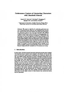
![How to move beyond lecture capture: [PDF]](https://m.moam.info/img/260x300/how-to-move-beyond-lecture-capture-pdf_648fd9a7098a9e5c1a8b4573.jpg)

