How to construct a volatility surface Aarhus Quant Day 17 jan 2014 Brian Huge Danske Markets
[email protected]
Outline • Motivation • Forward equation • Creating a volatility surface • Arbitrage free call prices • Short maturity expansion – Examples Local vol, SABR, ZABR
• Arbitrage in expansions • Local volatility vs FD volatility • Conclusion
References • Andreasen and Huge – Volatility Interpolation (Risk 2011) • Andreasen and Huge – Expanded forward volatility (Risk 2013) • • • •
Balland – Forward Smile (ICBI 2006) Carr – Local Variance Gamma (2008) Dupire, B. – Pricing with a Smile. (Risk 1994) Gatheral and Jacquier – Arbitrage-free SVI volatility surfaces, (Working paper 2013) • Hagan, Kumar, Lesniewski and Woodward – Managing Smile Risk (Risk 2002) • Nabben, R. – Decay Rates of the Inverse of Non-Symmetric Tridiagonal and Band Matrices. (J. Matrix Anal. Appl 1999)
Motivation 1/2 • Implied volatilities are quoted for discrete expiries and strikes • How can we extend this to a continuous surface in expiry and strike? – Reproduce quoted volatilities – Arbitrage free volatilities – Practical/fast implementation
• Parametric approaches like SSVI (Surface SVI) – – – –
simple formulas/implementation fast calculations give structure to the smile cannot fit all quotes
Motivation 2/2 • Non-parametric approach – fit all quotes – not much structure to the smile
• Volatility surface is – used for pricing and risk manage European options – input to a stochastic local volatility model • Method must be fast
Numerical example: Quotes SX5E • Market data 15 jan 2014 strikes
• Between 30 and 60 strikes for a given maturity • 8 different maturities
Forward equation 1/4 • Let c(T , k ) be the price of a call option with maturity T and strike k • Consider Dupire’s forward equation cT (T , k )
(T , k ) 2 2
ckk (T , k )
then the local volatility function is (T , k ) 2
cT (T , k ) ckk (T , k )
• For any function c with cT 0, ckk 0 there exists a local volatility function so c is an arbitrage free set of call prices
Forward equation 2/4 • Define the Laplace transform
L( g )(u ) eut g (t )dt 0
then integration by parts gives the (standard) relation L( gt )(u) uL( g )(u) g (0)
• I.e. the differential operator is changed to a finite difference operator • We will put a density on the maturity – Stochastic time – This is similar to the Variance Gamma model
Forward equation 3/4 • We will use an exponential density (VG uses gamma dist) 1 tT f (t ) e T
so the average time is the maturity T . (Variance is T 2.) • A set of call prices can now be calculated as
L(c (, k ))( T1 ) c(T , k ) f (t )c (t , k )dt T 0
where c is generated by ct (t , k )
• We find
(k )2 2
ckk (t , k )
c(T , k ) c(0, k ) ( k ) 2 ckk (T , k ) T 2
Forward equation 4/4 • This approach generates an arbitrage free set of call prices since the variance of the exponential distributions used are increasing in maturity • For the non-believers it is easily shown directly
1 tT ckk (T , k ) e ckk (t , k )dt 0 T 0
cT (T , k )
(k ) 2
2
e
t
T
ckk (t , k )dt
0
T
(k ) 2
2
te
t
T
ckk (t , k )dt
0
T
2
0
Creating a vol surface 1/2 • Let T1, T2 be quoted maturities • At quoted maturities we price by 1 (k )2 2 c(T1 , k ) c(0, k ) 1 T1 2 2 k 2 (k )2 2 c(T2 , k ) c(T1 , k ) 1 T2 2 2 k
• We calibrate the volatility functions 1,2 to match observed quotes at T1, T2 – E.g. piecewise constant or linear functions • We can choose 1,2 such that any number of quoted call
prices can be reproduced
Creating a vol surface 2/2 • In between quoted expiries e.g. T T1 we price
1 (k ) 2 2 c(T , k ) c(0, k ) 1 T 2 2 k • In general we price
0
T1
T2
• Fast since all call prices can be found by one stepping between quoted expiries • Need to show that the discrete state version is actually arbitrage free
Arbitrage free call prices 1/4 • We will discretize the state space by k ki ki1 then ( ki ) 2 kk c(T , ki ) c(0, ki ) 1 T 2
where
f (k k ) 2 f (k ) f (k k ) kk f (k ) k 2
• Stacking the equations we get a matrix equation ( I TD)C (T ) C (0)
• This is an implicit finite difference grid with C (T ) I TD C (0) 1
Arbitrage free call prices 2/4 0 z 1 0 D
0
0
0
2 z1
z1
0
z2
2 z2
z2
zn 2
2 zn 2
zn 2
0
zn 1
2 zn 1
0
0
0
0 zn 1 0
zi
( ki ) 2 2 k 2
• I TD is row diagonally dominant with negative off diagonals (not generally symmetric) 1 1 I TD I TD 1 1 hence it is a • is positive (Nabben), probability distribution. 1 • I TD is a probability distribution similar to the (discrete) Laplace distribution.
Arbitrage free call prices 3/4 1 x f cont ( x) e , xR 2
f disc ( x)
1 p x p , xZ 1 p
3 2.5 2
0.2
1.5 1 0.5 0 -3
-2
-1
0
1
2
3
Arbitrage free call prices 4/4 • We will now show that the implicit FD grid generates arbitrage free call prices • First, we will show that c(T , k ) 0 kk
DC(T ) D( I TD)1C(0) ( I TD)1 DC(0) 0 which is true for any convex function C (0). • Second, we show that cT (T , k ) 0 by differentiating the implicit FD equation wrt T ( I TD)CT (T ) DC (T ) 0
CT (T ) ( I TD) 1 DC (T ) 0 since DC (T ) 0 .
Numerical example: Local vol SX5E 15jan2014 1 0.9 0.8
0.9-1
0.7
0.8-0.9
0.6
0.7-0.8
0.5
0.6-0.7 0.5-0.6
0.4
0.4-0.5
0.3
0.810404 0.695414 0.580424 0.465435 0.350445 0.235455
0.2 0.1
7131.289
6761.886
6411.617
6079.492
5764.572
5465.965
5182.826
4914.353
4418.409
0.120465 4659.787
2333.796 2461.292 2595.753 2737.560 2887.114 3044.838 3211.178 3386.606 3571.617 3766.736 3972.513 4189.533
0
0.3-0.4 0.2-0.3 0.1-0.2 0-0.1
Calculation time • • • •
8 maturities Between 30-60 strikes for each maturity Total 365 quotes Calibration time < 0.05s
The opera house 1/2 •
The local volatility surface – is stable – without spikes
• •
However it looks like the opera house in the wings We can adjust for this by taking more FD steps n
TD c(T ) 1 c(0) n •
This will also generate arbitrage free prices n
TD Dc(T ) 1 Dc(0) 0 n TD cT (T ) 1 n •
n 1
Dc(0) 0
The algorithm will be n times slower than the 1 step
The opera house 2/2 0.3
0.25
0.2
n=1 n=2
0.15
n=3 n=100
0.1
0.05
0 0
5
10
15
20
25
30
14622.49
13501.16
12465.81
11509.87
10627.23
9812.271
9059.811
8365.055
7723.576
7131.289
6584.423
6079.492
5613.283
5182.826
4785.378
4418.409
4079.58
3766.736
3477.881
3211.178
2964.927
2737.56
2527.629
2333.796
2154.828
The opera house n=1
1
0.9
0.8
0.7 0.9-1
0.8-0.9
0.6 0.7-0.8
0.5
0.6-0.7
0.4 0.5-0.6
0.3 0.4-0.5
0.2 0.3-0.4
0.1
0 0.695414 0.561259 0.427105 0.29295
0.158795
0.024641
0.2-0.3
0.1-0.2
0-0.1
14622.49
13501.16
12465.81
11509.87
10627.23
9812.271
9059.811
8365.055
7723.576
7131.289
6584.423
6079.492
5613.283
5182.826
4785.378
4418.409
4079.58
3766.736
3477.881
3211.178
2964.927
2737.56
2527.629
2333.796
2154.828
The opera house n=2
1
0.9
0.8
0.7 0.9-1
0.8-0.9
0.6 0.7-0.8
0.5
0.6-0.7
0.4 0.5-0.6
0.3 0.4-0.5
0.2 0.3-0.4
0.1
0 0.695414 0.561259 0.427105 0.29295
0.158795
0.024641
0.2-0.3
0.1-0.2
0-0.1
14622.49
13501.16
12465.81
11509.87
10627.23
9812.271
9059.811
8365.055
7723.576
7131.289
6584.423
6079.492
5613.283
5182.826
4785.378
4418.409
4079.58
3766.736
3477.881
3211.178
2964.927
2737.56
2527.629
2333.796
2154.828
The opera house n=10
1
0.9
0.8
0.7 0.9-1
0.8-0.9
0.6 0.7-0.8
0.5
0.6-0.7
0.4 0.5-0.6
0.3 0.4-0.5
0.2 0.3-0.4
0.1
0 0.695414 0.561259 0.427105 0.29295
0.158795
0.024641
0.2-0.3
0.1-0.2
0-0.1
Short Maturity Expansion 1/4 • Consider the stochastic volatility model ds ( s, z )dW dz ( s, z )dZ dWdZ ( s, z )dt
• Several model choices can fit the same smile – E.g. a pure local vol model can fit a smile generated by the SABR model • Let c(t ) be the time t price of a European call option c(t ) Et [ s(T ) k ]
Short Maturity Expansion 2/4 • We will use Bachelier’s option pricing formula x x g (t , s, v) ( s k ) v sk x v T t
to find the implied normal volatility as c(t ) g (t , s(t ), v(t ))
• Now, v is an implicit given function of the state variables s, z , hence a stochastic variable • An Ito expansion yields
Short Maturity Expansion 3/4 dc gt dt g s ds g v dv
• Use the properties
1 1 g ss ds 2 g sv dsdv g vv dv 2 2 2
v2 gt g g ss , g v v g ss , g sv xg ss , g vv x 2 g ss 2
to find
v2 dc g s ds g ss dx 2 dt 2 dv 2 v
• Next we take expectation on both sides and use that Et [dc] 0 to find 2 dx dt 2 Et [dv] 0 v
(1)
Short Maturity Expansion 4/4 • For short maturity or 0 we get the condition that x needs to be a unit diffusion dx 2 2 xs2 2 xs xz 2 xz2 1 dt
, x( s k ) 0
• This is the short maturity arbitrage condition on the implied volatility sk ln( s / k ) v
x
or
vBS
x
• This is the Eikonal equation. It is a non-linear first order PDE on the diffusion rather than the linear second order PDE on the drift we typically use in finance • This derivation follows Balland (2006) and Andreasen and Huge(2013)
Local volatility model For the pure local volatility model
ds ( s )dW
x is just a function of spot and we need to solve xs 1
with initial condition x( s k ) 0 Hence, s 1 du (u ) k
x
with implied volatility v s
sk x s
sk s
u du k
1
Local (Dupire) volatility 1/2 • 2 models that produces the same function x will have the same smile (or implied volatilities) • For a given x we can define the local volatility function as x (k ) k
1
then the local volatility model ds ( s )dW will reproduce the function x . • Andersen and Ratcliffe suggests an implied volatility expansion in cases with time homogeneous local volatility
Local (Dupire) volatility 2/2 • The expanded local volatility can also be written in terms of the smile 1 v2 x (k ) v ( s k )vk k
• For 0 we have
c v2 2 ckk v ( s k )vk
i.e. the Dupire local volatility.
Sabr 1/3 • Log normal stochastic volatility
ds ( s) zdW dz zdZ dWdZ dt
• Inspired by the local volatility model we define s
1 1 y du z k u
which follows dy
dt
y 1 dz ds z z s
dt ydZ dW
dt 1 2 y y 2
2
1 2
dB
Sabr 2/3 • We can solve the Eikonal equation with y
x 1 2 u u 2
1 2 2
du
0
1 2 y 2 y 2 y log 1 1
and the implied volatility is v
sk 1 2 y 2 y 2 y log 1
• This expression is also found in Hagan et al
Sabr 3/3 • The local volatility is 1
1 x 2 2 2 y k 1 2 y y k k
1 2 y y 2
2
1 2
1
z k
• By deriving the local volatility we have reduced the 2d PDE to a 1d PDE
CEV stochastic volatility 1/4 • We now extend the stochastic volatility to a CEV process ds z s dW dz z dZ dWdZ dt
• The motivation for this extension is better control with the wings of the smile • Both parameters , in the stochastic vol process control the curvature of the smile • controls the far out of the money volatilities – Extrapolation to low deltas in FX – CMS pricing
CEV stochastic volatility 2/4 0.7 0.6 0.5 g=1.5
0.4
g=1 0.3
g=0.5 g=0
0.2 0.1 0 0
1
2
3
4
5
6
7
CEV stochastic volatility 3/4 • Define
x wf ( y ) s
1 1 w du z k u yz
Then dx
2
s
1 k u du
dt f y yf ' y dW y f y 2 yf ' y dZ
with quadratic variation 2 dx 2 f y yf ' y 2 y f y 2 yf ' y f y yf ' y dt
2 y 2 f y 2 yf ' y
2
CEV stochastic volatility 4/4 • We conclude that f should solve the ODE 2 f y yf ' y 2 y f y 2 yf ' y f y yf ' y 2 y 2 f y 2 yf ' y 1 2
• The local volatility function is x k k
1
wk f y wf ' y yk z k f y yf ' y
1
1
Local volatility vs FD volatility 1/9 • The short term expansion is a simple way to find approximations for implied volatility • However, the short term expansion can still lead to arbitrages – both for high and low strikes
10Y density with short term SABR expansion 5 4 3 2 1 0 -1
0
0.5
1
1.5
2
Local volatility vs FD volatility 2/9 • We still need a way to price call options which garanties no arbitrage • Could use Dupire’s forward equation to price ct
(k ) 2 2
ckk
with the expanded local volatilities • This would be rather slow • Instead we will use the 1 step FD grid which garanties arbitrage free call prices • Compared to the original 1 step FD method we will add some structure to the implied volatility smile – control over the wings – Easier interpolation between maturities with few strikes
Local volatility vs FD volatility 3/9 • Remember that the 1 step FD is like a Laplace transformation • Assume that call prices are generated by a Gaussian process then the Laplace transform is
t T
t T
e ckk T , k e ckk t , k dt 0 0 v t
sk n dt v t
T s k e 2 2v
2 2
v T
• The abs value in the exponent gives a peak in atm which is difficult to approximate with a Gaussian distribution
Local volatility vs FD volatility 4/9 8
7 6 5 Gaussian
4
Laplace
3 2 1 0 0
0.5
1
1.5
2
Local volatility vs FD volatility 5/9 • Must find an adjustment that compensates for the 1 step algorithm • For a Gaussian distribution we can calculate the approximation error • We would like to find an ”FD volatility” such that option prices generated by the 1 step FD grid are approximately the same as option prices generated by the forward equation cT
(k ) 2 2
ckk ckk
2 c 2 T (k )
• So we replace ckk in the 1 step FD equation Tii (k ) 2 c(Ti , k ) c(Ti 1 , k ) ckk (Ti , k ) 2
and solve for i
Local volatility vs FD volatility 6/9 i (k ) 2 i (k ) 2 i (k ) 2
c(Ti , k ) c(Ti 1 , k ) Ti cT (Ti , k ) g (Ti , k , v) g (Ti 1 , k , v) Ti gT (Ti , k , v) FD adjustment
• For i 1 ( ) ( k ) ( k ) 2 1 ( ) 2
2
,
sk v T
FD adjustment
• We will use our expansion to approximate the volatility in the FD adjustment
Local volatility vs FD volatility 7/9 2.5 2 1.5 Adjustment Density
1 0.5 0 -8
-6
-4
-2
0
2
4
6
8
Local volatility vs FD volatility 8/9 0.45 0.4 0.35
0.3 0.25
2d FD
0.2
1 step FD
0.15 0.1 0.05 0 0
1
2
3
4
5
Local volatility vs FD volatility 9/9 • FD adjustment with Ti 1 2.5
2
1.5 T(i-1)=0 T(i-1)=0.5 1
T(i-1)=1
0.5
0 0.7
0.8
0.9
1
1.1
1.2
1.3
Conclusion • We have derived a method for interpolating and extrapolating quoted volatilities (both in maturity and strike) to a full surface – – – – –
Fast calibration Reproduces all quoted volatilities Arbitrage free Stable and fast algorithm for pricing European options Fast enough to use as input to a stochastic local vol model
• We can extend the method to use a parametric form with a clear link to known models like SABR • We can control the extrapolation explicitly • The local vol function can be chosen independently of the stochastic volatility process