How To Make a Greedy Heuristic for the Asymmetric Traveling Salesman Problem Competitive Boris Goldengorin∗ and Gerold J¨ager†
Abstract It is widely confirmed by many computational experiments that a greedy type heuristics for the Traveling Salesman Problem (TSP) produces rather poor solutions except for the Euclidean TSP. The selection of arcs to be included by a greedy heuristic is usually done on the base of cost values. We propose to use upper tolerances of an optimal solution to one of the relaxed Asymmetric TSP (ATSP) to guide the selection of an arc to be included in the final greedy solution. Even though it needs time to calculate tolerances, our computational experiments for the wide range of ATSP instances show that tolerance based greedy heuristics is much more accurate and faster than previously reported greedy type algorithms.
1
Introduction
Perhaps the most famous classic combinatorial optimization problem is called the Traveling Salesman Problem (TSP) ([20]). It has been given this picturesque name because it can be described in terms of a salesperson who must travel to a number of cities during one tour. Starting from his (her) home city, the salesperson wishes to determine which route to follow to visit each city exactly once before returning to his home city so as to minimize the total length tour. The length (cost) of traveling from city i to city j is denoted by c(i, j). These costs are called symmetric if c(i, j) = c(j, i) for each pair of cities i and j, and asymmetric otherwise. A TSP instance is defined by all non-diagonal entries of the n × n matrix C = ||c(i, j)||. There have been a number of applications of TSP that have nothing to do with salesman. For example, when a truck leaves a distribution center to deliver goods to a number of locations, the problem ∗ Corresponding author. Department of Econometrics and Operations Research, University of Groningen, P.O. Box 800, 9700 AV Groningen, The Netherlands; Fax. +31-50-363-3720, Email:
[email protected] and Department of Applied Mathematics, Khmelnitsky National University, Ukraine † Computer Science Institute, Martin-Luther-University Halle-Wittenberg, VonSeckendorff-Platz 1, 06120 Halle (Saale), Germany, E-mail:
[email protected]
1
of determining the shortest route for doing this is a TSP. Another example involves the manufacture of printed circuit board, the problem of finding the most efficient drilling sequence is a TSP. More applications to Genome Sequencing, Starlight Interferometer Program, DNA Universal Strings, Touring Airports, Designing Sonet Rings, Power Cables, etc are indicated at ([19]). Computer scientists have found that the ATSP is among certain type of problems, called NP-hard problems which are especially intractable, because the time it takes to solve the most difficult examples of an NP-hard problem seems to grow exponentially as the amount of input data increases. Surprisingly, powerful algorithms based on the branch-and-cut (b-n-c) ([21]) and branch-andbound (b-n-b) ([5]) approaches have succeeded in solving to optimality certain huge TSPs with many hundreds (or even thousands) of cities. The fact that the TSP is a typical NP-hard optimization problem means, that solving instances with a large number of cities is very time consuming if not impossible. For example, the solution of the 15112-city TSP was accomplished in several phases in 2000/2001, and used a total of 22.6 years of computer time, adjusted to a 500 MHz, EV6 Alpha processor ([18]). A heuristic is a solution strategy that produces an answer without any formal guarantee as to the quality ([20]). Heuristics clearly are necessary for NP-hard problems if we expect to solve them in reasonable amounts of computer time. Heuristics also are useful in speeding up the convergence of exact optimization algorithms, typically by providing good starting solutions. A metaheuristic is a general solution method that provides both a general structure and strategy guidelines for developing a specific heuristic method to fit a particular kind of problem. Heuristics can be classified into several categories, namely construction, improvement, partitioning and decomposition, and specialized heuristics ([25]). A construction heuristic for the TSP build a tour without an attempt to improve the tour once constructed. Construction heuristics are the fastest heuristics among all of the above mentioned categories of heuristics ([6],[7]). They can be used to create approximate solutions for the TSP when the computing time is restricted, to provide good initial solutions for exact b-n-c or b-n-b algorithms ([21],[5]). The Greedy Algorithm (GR) is one of the fastest construction type heuristic in combinatorial optimization. Computational experiments show that the GR is a popular choice for tour construction heuristics, work at acceptable level for the Euclidean TSP, but produce very poor results for the general Symmetric TSP (STSP) and Asymmetric TSP (ATSP) ([6]-[8]). The experimental results for the asymmetric TSP presented in [7] led its authors to the conclusion that the greedy algorithm “might be said to self-destruct” and that it should not be used even as “a general- purpose starting tour generator”. A numerical measure for evaluation of heuristics that compares heuristics according to their so called domination number is suggested in ([9]). The domination number of a heuristic A for the TSP is the maximum integer d(n) such that, for every instance I of the TSP on n cities, A produces a tour h which is not worse than at least d(n) tours in I including h itself. Theorem 2.1 in [13] (see also [14]) on the greedy algorithm for the ATSP confirms the above 2
conclusion: for every n > 1 there exist instances of the asymmetric TSP with n vertices for which the greedy algorithm produces the unique worst tour. In the abstract of [1] the authors send the following message: “The practical message of this paper is that the greedy algorithm should be used with great care, since for many optimization problems its usage seems impractical even for generating a starting solution (that will be improved by a local search or another heuristic).” Note that all these negative conclusions are drawn for the cost based greedy (CBG) type heuristics. There are various heuristic methods based on tolerances and related to a specific mathematical programming problem, for example to the well known transportation problem, available to get an initial basic feasible solution, such as northwest corner rule, best cell method, etc. Unfortunately, there is no reason to expect the basic feasible solution provided by the northwest corner rule to be particularly close to the optimal solution. Therefore, it may be worthwhile to expand a little more effort on obtaining a promising initial basic feasible solution in order to reduce the number of iterations required to reach the optimal solution. One procedure which is designed to do this is Vogel’s Approximation Method (VAM) [23]. The VAM is based on the use of the “difference” associated with each row and column in the original instance C. A row or column “difference” is defined as the arithmetic difference between the smallest and next-to-the smallest element in that row or column. This quantity provides a measure of the proper priorities for making allocations to the respective rows and columns, since it indicates the minimum unit penalty incurred by failing to make an allocation to the smallest cell in that row or column [16]. Such a difference is also called the regret for that row(column) [2] because it represents the minimum penalty for not choosing the smallest cost in the row (column). The element with the smallest cost in the row (column) with the largest regret is selected in VAM for starting the transportation simplex algorithm. A similar idea applied to rows is used for the MAX-REGRET heuristic for solving the three-index assignment problem [2]. In this paper we generalize the above mentioned “differences” within the notion of upper tolerances and apply them within a framework of branch-and-bound algorithms for solving the ATSP by greedy type heuristics. Although the concept of tolerances has been applied for decades (in sensitivity analysis; see e.g. [12] and [17]), only Helsgaun’s version of the Lin-Kernighan heuristic for the STSP applies tolerances; see [15]. As easy to see the VAM, MAX-REGRET and Helsgaun’s version of the Lin-Kernighan heuristics are not embedded in a unified framework called a metaheuristic for solving different combinatorial optimization problems. Let us remind that a metaheuristic is a general solution method that provides both a general structure and strategy guidelines for developing a specific heuristic method to fit a particular kind of problem. All above mentioned heuristics are special cases of our metaheuristic. For example, our metaheuristic applied to the ATSP leads to a family of heuristics including our R-RTBG heuristic which is an analogy of MAX-REGRET heuristic for the three-index assignment problem [2]. To our best knowledge such a family of heuristics does not discussed in the available literature. 3
Currently, most of construction heuristics for the TSP including the GR delete high cost arcs or edges and save the low cost ones. A drawback of this strategy is that costs of arcs and edges are no accurate indicators whether those arcs or edges are included or excluded in a ‘good’ TSP solution. In ([11]) and ([26]), it is shown that tolerances are better indicators, and they have been successfully applied for improving the bounds and branching rules within the framework of b-n-b algorithms. A tolerance value of an edge/arc is the cost of excluding or including that edge/arc from the solution at hand. In this paper we present a tolerance based metaheuristic within a framework of branch-andbound paradigm and apply it for solving the ATSP. Our paper is organized as follows. In the next section we embed the GR for the ATSP in a metaheuristic based on branch-and-bound paradigm and tolerances. Here we define the Contraction Problem (CP) of finding an arc for contraction by the GR and show that an optimal solution to a natural relaxation of the Assignment Problem (AP) can be used as an extension of an optimal solution to CP. In Section 3 we briefly report on previous work related to tolerances in combinatorial optimization and discuss the computational complexities of tolerance problems for the AP and Relaxed AP. In Section 4 we describe a set of tolerance based greedy algorithms with different relaxations of the ATSP and report the results of computational experiments with them in Section 5. The conclusions and future research directions appear in Section 6.
2
The Greedy Algorithm within a framework of a metaheuristic
Let us remind the GR for the ATSP as it is described in ([8]). We consider the entries of the n × n matrix C as costs (weights) of the corresponding simple weighted complete digraph G = (V, E, C) with V = {1, . . . , n} vertices and E = V × V arcs such that each arc (i, j) ∈ E is weighted by c(i, j). The GR finds the lightest arc (i, j) ∈ E and contracts it updating the costs of C := Cp till C consists of a pair of arcs. The contracted arcs and the pair of remaining arcs form the “Greedy” tour in G. We shall address the GR in terms of the b-n-b framework for solving the ATSP. A b-n-b algorithm initially solves a relaxation of the original NP-hard problem. In case of the ATSP, the Assignment Problem (AP) is a common choice. The AP, in terms of the ATSP, is the problem of assigning n city’s outputs to n city’s inputs against minimum cost; an optimal solution of the AP is called a minimum cycle cover. In terms of the ATSP an AP feasible solution requires that each city will be visited exactly once without necessarily creating a single (Hamiltonian) cycle. If the minimum cycle cover at hand is a single tour, then the ATSP instance is solved; otherwise, the problem is partitioned into new subproblems by including and excluding arcs. In the course of the process, a search tree is generated in which all solved subproblems are listed. B-n-b algorithms comprise two major ingredients: a branching rule and a lower
4
bound. The objective of branching rule is to exclude the infeasible solutions to the ATSP found for its relaxation. A lower bound is applied to fathom as many vertices in the search tree as possible. A subproblem is fathomed if its lower bound exceeds the value of the best ATSP solution found so far in the search tree. For sake of simplicity, we consider only the so called binary branching rules ([29]), i.e. such a branching rule which either include or exclude a selected arc from the current optimal solution to a relaxation of the ATSP. We present the execution of the GR by a single path of the corresponding b-n-b search tree such that the lower bound is equal to the Glover et al.’s Contraction Problem (CP) ([8]) and the branching rule is defined by a lightest arc in the given ATSP instance. Since at each iteration the GR contracts a single lightest arc, i.e. creates a subproblem which includes that arc in the unknown GREEDY solution, it means that the GR discards the another subproblem in which the same arc is prohibited. Thus the GR can be represented by a single path in a search tree consisting only vertices (subproblems) related to each inclusion of an arc from the optimal solution of a relaxed ATSP. We define the CP as follows: min {c(i, j) : i, j ∈ V } = c(i0 , j0 ), We also use the following two simple combinatorial optimization problems related to either the ATSP or CP, namely either the Assignment Problem (AP) or the Relaxed AP (RAP), respectively. We define the AP as follows: n n o X min a(π) = c(i, π(i)) : π ∈ Π = a(π0 ), i=1
here a feasible assignment π is a permutation which maps the rows V of C onto P the set of columns V of C and the cost of permutation π is a(π) = (i,j)∈π c(i, j); Π is the set of all permutations, and π is called feasible if a(π) < ∞. Now we define the RAP. A feasible solution θ to the RAP is a mapping θ of the rows V of C into the columns V of C with a(θ) < ∞. We denote the set of feasible solutions to the RAP P by Θ. It is clear that Π ⊂ Θ. The RAP is the problem of finding a(θ0 ) = i∈V min{c(i, j) : j ∈ V }. Further we will treat a feasible solution θ as a set of n arcs. As easy to see an optimal solution (arc) (i0 , j0 ) to the CP is included in an optimal solution θ0 to the RAP, i.e. (i0 , j0 ) ∈ θ0 . So, one may to consider θ0 as an extension of an optimal solution to the CP. If the set of optimal solutions (arcs) to the CP has more than one arc and these arcs are located in pairwise distinct rows of C, then at most n arcs will be included in an optimal solution to the RAP. The relationship between the optimal values of CP and RAP is described in the following lemma. Lemma 1 For any n > 1 we have that c(i0 , j0 ) ≤ a(θ0 )/n. P P Proof. a(θ0 ) = i∈V min{c(i, j) : j ∈ V } ≥ i∈V c(i0 , j0 ) = nc(i0 , j0 ).
For sake of completeness we define the ATSP as follows. A feasible solution π to the AP is called a cyclic permutation and denoted by h if the set of its arcs 5
represents a Hamiltonian cycle in G. The whole set of Hamiltonian cycles in G is denoted by H. Thus, the ATSP is the problem of finding min{a(h) : h ∈ H} = a(h0 ). It is clear that H ⊂ Π ⊂ Θ implies that nc(i0 , j0 ) ≤ a(θ0 ) ≤ a(π0 ) ≤ a(h0 ). Note, that the computational complexities for finding an optimal solution to the CP, RAP, and AP are O(n2 ), O(n2 ), and O(n3 ), respectively.
3
Tolerances for the RAP and AP
The second concept we have built on is the tolerance problem for a relaxed ATSP. The tolerance problem for the RAP is the problem of finding for each arc e = (i, j) ∈ E the maximum decrease l(e) and the maximum increase u(e) of the arc cost c(e) preserving the optimality of θ0 under the assumption that the costs of all other arcs remain unchanged. The values l(e) and u(e) are called the lower and the upper tolerances, respectively, of arc e with respect to the optimal solution θ0 and the function of arc costs c. In the following portion we consider a combinatorial minimization problem defined on the ground set E: min{a(S) : S ∈ D} = a(S ∗ ), P with an additive objective function a(S) = e∈S c(e), the set of feasible solutions D ⊂ 2E , set of optimal solutions D ∗ such that S ∗ ∈ D∗ . For each e ∈ E, ∗ ∗ D+ (e) and D− (e) are the sets of optimal solutions containing e and not contain∗ ∗ ∗ ∗ (e) = ∅. If D = Π then we (e) ∪ D− (e) and D+ (e) ∪ D− ing e such that D∗ = D+ have the AP, and if D = Θ then we have the RAP. As shown [11],[10] for each ∗ e ∈ S ∗ the upper tolerance uS ∗ ∈D (e) = a(S) − a(S ∗ ) for each S ∈ D− (e), and ∗ means the upper tolerance of an element e ∈ S with respect to the set of feasible solutions D. Similarly, the lower tolerance lS ∗ ∈D (e) = a(S) − a(S ∗ ) for each ∗ S ∈ D+ (e), and means the lower tolerance of an element e ∈ / S ∗ with respect to the set of feasible solutions D. If one excludes an element e from the optimal solution S ∗ , then the objective value of the new problem will be a(S ∗ )+uS ∗ ∈D (e). The same holds for the lower tolerance if the element e ∈ E \ S ∗ is included. So a tolerance-based algorithm knows the cost of including or excluding elements before it selects the element either to include or to exclude. Moreover, based on the upper tolerances one may describe the set of optimal solutions D ∗ to RAP as follows ([11],[10]): (i) if u(e) > 0 for all e ∈ S ∗ , then |D∗ | = 1; (ii) if u(e) > 0 for e ∈ R ⊂ S ∗ and u(e) = 0 for e ∈ S ∗ \ R, then |D∗ | > 1 and ∩D∗ = R. (iii) if u(e) = 0 for all e ∈ S ∗ , then |D∗ | > 1 and ∩D∗ = ∅. As shown in ([11],[26],[15]) the average percentage of common arcs in corresponding AP and ATSP optimal solutions varies between 40% and 80%, and we claim that the average percentage of common arcs in corresponding RAP and ATSP optimal solutions varies between 20% and 50%. Moreover, an arc 6
with the largest upper tolerance from an optimal AP solution will appear in an optimal ATSP solution in average 10 times more often than a lightest arc from the optimal AP solution. Similarly, an arc with the largest upper tolerance from an optimal RAP solution will appear in an optimal ATSP solution in average 15 times more often than a lightest arc from the optimal RAP solution. These results confirm that predictions based on upper tolerances are clearly better than predictions based on costs ([11],[26],[15]). Hence, our branching rule for the tolerance based algorithms will use an arc with the largest upper tolerance w.r.t. either the RAP or the AP. It is important to mention that the time complexity of the tolerance problem for a Polynomially Solvable (PS) problem (for example, either the RAP or AP) defined on the set of arcs E ([3],[27]) is at most O(|E|g(n)|), assuming that the time complexity of PS problem is equal to g(n). Hence, the time complexities of solving the tolerance problems for RAP and AP are at most O(n4 ) and O(n5 ), respectively, because the time complexities of solving the RAP and AP are O(n2 ) and O(n3 ), respectively. Recently, Volgenant ([28]) has suggested an O(n3 ) algorithm for solving the tolerance problem for AP. Let us show that the time complexity of tolerance problem for the RAP is O(n2 ). For finding the optimal value a(θ0 ) of RAP we should find in each i-th row of C its smallest value min{c(i, j) : j ∈ V } = c[i, j1 (i)] and for computing the upper tolerance u[i, j1 (i)] of the arc [i, j1 (i)] it is enough to know a pair of smallest values in the same row i, i.e. c[i, j1 (i)] and c[i, j2 (i)] = min{c(i, j) : j ∈ V \{j1 (i)}}. Thus, u[i, j1 (i)] = c[i, j2 (i)]−c[i, j1 (i)] will be computed in O(n) time with O(1) space complexity. For computing all lower tolerances for entries in i-th row it is enough to reduce each entry of the i-th row by the smallest value c[i, j1 (i)], i.e. l(i, j) = c(i, j) − c[i, j1 (i)] for j ∈ V \ {j1 (i)} and l[i, j1 (i)] = ∞. Again, such a reduction can be done in O(n) time and the result can be stored in i-th row of C. Now we are able to solve the RAP and compute all tolerances in O(n2 ) time and O(n) space complexities. Note that the AP can be solved in O(n3 ) time and computing all upper tolerances for an optimal AP solution w.r.t. the AP needs also O(n3 ) time, but an optimal AP solution is a feasible RAP solution. Hence, with purpose to decrease the computational complexity of upper tolerances for an optimal AP solution from O(n3 ) time to O(n2 ) time, we have decided to compute the upper tolerances for an optimal AP solution w.r.t. the RAP as follows. Let π0 = {[i, jk (i)] : i = 1, . . . , n} be a set of arcs [i, jk (i)] from an optimal AP solution. Then we define the upper tolerance uπ0 ∈Θ [i, jk (i)] of an arc [i, jk (i)] from an optimal AP solution w.r.t. the RAP as follows: uπ0 ∈Θ [i, jk (i)] = c[i, jk+1 (i)] − c[i, jk (i)], for k = 1, . . . , n − 1; uπ0 ∈Θ [i, jn (i)] = c[i, jn (i)] − c[i, jn−1 (i)], for k = n. Here, for each row i of C we have ordered all its entries in a non-decreasing order, i.e. c[i, j1 (i)] ≤ c[i, j2 (i)] ≤ . . . ≤ c[i, jn−1 (i)] ≤ c[i, jn−1 (i)].
7
4
A tolerance based metaheuristic
Let us explain our enhancements of tolerance based greedy algorithms compared to the cost based GR in the framework of b-n-b algorithms. Our first enhancement is based on an improved lower bound for the ATSP (either the RAP or AP) compared to the CP. Our second enhancement is based on an improved branching rule which uses the largest upper tolerance of an arc from an optimal solution to either the RAP or AP instead of a lightest arc from an optimal solution to the CP. Note that by using the RAP instead of CP we may expect the quality improvement of a RAP based greedy solutions without essential increasing of the computing times. Since the time complexity of AP is O(n3 ), the question whether we may reach further improvements by the AP based greedy algorithm without essential increment of computing times will be answered by means of computational experiments. Now we are ready to present two Tolerance Based Greedy (TBG) algorithms, namely the X-Y TBG algorithms with X, Y ∈ {R, A} in the same framework as the original GR. Here the first letter “X” stands for a relaxation of the ATSP and the second letter “Y” stands for the tolerance problem of one of the relaxations of ATSP. Our first algorithm is the RAP Tolerance Based Greedy (R-RTBG) algorithm. The R-RTBG algorithm recursively finds an arc (i, j) ∈ E with the largest upper tolerance from an optimal RAP solution, and contracts it updating the costs of C := Cp till C consists of a pair of arcs. The index p in Cp stands for a new vertex p found after each contraction of the arc (i, j). The contracted arcs and the pair of remaining arcs form the “R-RTBG” tour in G. The R-RTBG algorithm runs in O(n3 ) time since a single contraction needs O(n2 ) time. Note that if at the current iteration after a single contraction the deleted column does not include either a lightest out-arc or a corresponding upper tolerance, then at the next iteration of R-RTBG algorithm we preserve all lightest out-arcs and the corresponding upper tolerances. Otherwise, at the next iteration the rows containing either a lightest out-arc or a corresponding upper tolerance will be updated.
8
Figure 1: Example: 6 × 6 matrix, class 8.
GR A
1
6 (1)
R - R TBG
2
1
6 (1)
2
13 (6)
12 (1)
2
3
5
6
4
5
13 (0)
3
13 (6) 13 (5)
13 (6)
1
6
13 (6) 6
A - R TBG
7 (0)
35 ()
18 (1) 3
4
4
5
19 (5)
B
1
1
2
4
2
13 (0)
12 (1)
5
1
7 (0)
12 (1) 7 (0) 6
3
6
3 13 (6)
19 (6) 5
C
4
1
2
18 (1)
4
13 (0) 5
18 (1)
4
6x6 cost matrix, class 8
3
19 (16) 2
1
3
4 1
6
6
4
2
13 (22)
24 (1) 7 (0)
3
5
1
2
3
4
5
6
1
66
7
7
7
7
2
35
12
13
13
13
3
35
13 13
18
19
19
4
35
13
19
24
25
5
35
13 13
19
25
30
6
216
13 13
19
25
31
5
7
E
216 6
1
2
3 30
306
19 (6) 3
2
25 (6) 6
D
18 (1)
7 (0) 1
5
4
19 (6)
5
3
6
6
2
18 (1)
4
5
1
6
4
2
5
3
35
112
105
For example (see the R-RTBG algorithm in Fig. 1), after first contraction on the iteration A we delete the second column from the 6 × 6 costs matrix together with the minima attained on the arcs (1, 2), (3, 2), (5, 2), (6, 2), and preserve the minimum attained on the arc (2, 3) in the third column. Hence, on the next iteration B the R-RTBG algorithm updates the minima and upper tolerances in rows 1, (4, 2), 5, 6 and preserves the minimum c[3, (4, 2)] = 12 and its upper tolerance u[3, (4, 2)] = 1. Here p = (4, 2) is a new vertex representing the contracted arc (4, 2). This book-keeping technique (for preserving either a lightest out-arc or a corresponding upper tolerance) incorporated in the RRTBG algorithm explains why in average we have reduced the PC times of R-RTBG compared to GR (see Table 1). Our second algorithm is the A-RTBG. The choice of the AP as the ATSP relaxation can be motivated as follows. The out-degree of each vertex in a graph representing an optimal RAP solution is equal to one and the in-degree of each vertex can be an arbitrary number between 0 and n − 1 such that the sum of 9
in-degrees of all vertices is equal to n (see iteration A of the R-RTBG in Fig. 1). The in-degree and out-degree for each vertex in the graph representing an optimal AP solution are equal to one (see iteration A of the A-RTBG in Fig. 1). Hence, the structural distinctions between the graphs of a feasible ATSP tour and a feasible RAP solution are worse compared to the structural distinctions between the graphs of a feasible ATSP tour and a feasible AP solution (see Fig. 1). Since the AP can be solved in O(n3 ) time and computing all upper tolerances to an optimal AP solution needs also O(n3 ) time, in the AP with RAP Tolerance Based Greedy (A-RTBG) algorithm we have decided to use an optimal AP solution as a better approximation of the unknown optimal ATSP solution. Note that each optimal AP solution is a feasible RAP solution. Therefore, with purpose to decrease the computational complexity of upper tolerances for an optimal AP solution from O(n3 ) time to O(n2 ) time, we have decided to compute the upper tolerances of RAP for the optimal AP solution instead of upper tolerances for the optimal AP solution itself. The A-RTBG algorithm recursively finds an arc (i, j) in an optimal AP solution with the largest upper tolerance from the tolerance RAP, and contracts it updating the costs of C := Cp till C consists of either a hamiltonian cycle or a pair of arcs. The contracted arcs and the pair of remaining arcs form the “ARTBG” tour in G. The A-RTBG algorithm runs in O(n4 ) time, since a single contraction needs O(n3 ) time. A slight modification of the A-RTBG algorithm based on upper and lower tolerances is denoted by A-R1 TBG algorithm and contracts an arc with the largest tolerance chosen from all tolerances as follows. Each lower tolerance is used with a negative sign and each upper tolerance with a positive sign. Hence, in the A-R1 TBG algorithm all involved tolerances have finite numbers. The distinctions in behavior of the GR, R-RTBG, and A-RTBG by means of the 6 × 6 numerical example taken from class 8 are illustrated in Fig. 1. The numbers 1, 2, ..., 6 on the left side of the vertical line and above the horizontal line in the 6 × 6 costs matrix are the numbers of cities. The same numbers are indicated as cycled numbers for vertices (cities). An optimal RAP (respectively, AP, ATSP) solution is indicated in the 6 × 6 costs matrix by cycled (respectively, squared, red) entries. A blue(yellow) vertex is an out-(in-) vertex before contraction and a red arc is an arc chosen for contraction. Each red arc after contraction is oriented from left to right and represented by two red neighboring vertices. If an end of a contracted sequence of arcs (path) is chosen for contraction, then the corresponding end became either blue or yellow. The numbers x(y) along each arc are the weight x (respectively, upper tolerance y) of the arc for GR, R-RTBG, and A-RTBG, where the upper tolerance y is computed w.r.t. the RAP. A bold letter on the left side corresponds to the current iteration number for each algorithm. The GR, R-RTBG, A-RTBG algorithms output greedy solutions with values 306, 112, 105 (optimal value), respectively. Fig. 1 shows that the A-RTBG algorithm needs less iterations (contractions) than the A-RTBG algorithm and returns a greedy solution at the second iteration (B) since all depicted arcs are arcs from an optimal AP solution which is a Hamiltonian cycle. 10
5
Computational experiments
The algorithms were implemented in C under Linux and tested on an AMD Opteron(tm) Processor 242 1.6 GHz machine with 4 GB of RAM. We test all four greedy algorithms GR, R-RTBG, A-RTBG, and A-R1 TBG on the following 8 classes of instances. The classes from 1 to 7 are exactly the classes from ([8]) and class 8 is the class of GYZ instances introduced in ([13]) for which the domination number of GR algorithm for the ATSP is 1 (see Theorem 2.1 in [13]). The exact description of the 8 classes is as follows. 1 All asymmetric instances from TSPLIB ([24]) (26 instances). 2 All symmetric instances from TSPLIB with dimension smaller than 3000 (99 instances). 3 Asymmetric instances with c(i, j) randomly and uniformly chosen from {0, 1, · · · , 100000} for i 6= j, 10 for each dimension 100, 200, · · · , 1000 and 3 for each dimension 1100, 1200, · · · , 3000 (160 instances). 4 Asymmetric instances with c(i, j) randomly and uniformly chosen from {0, 1, · · · , i · j} for i 6= j, 10 for each dimension 100, 200, · · · , 1000 and 3 for each dimension 1100, 1200, · · · , 3000 (160 instances). 5 Symmetric instances with c(i, j) randomly and uniformly chosen from {0, 1, · · · , 100000} for i < j, 10 for each dimension 100, 200, · · · , 1000 and 3 for each dimension 1100, 1200, · · · , 3000 (160 instances). 6 Symmetric instances with c(i, j) randomly and uniformly chosen from {0, 1, · · · , i · j} for i < j, 10 for each dimension 100, 200, · · · , 1000 and 3 for each dimension 1100, 1200, · · · , 3000 (160 instances). 7 Sloped plane instances with given xi , xj , yi , yj randomly and uniformly chosen from {0, 1, · · · , i · j} for i 6= j and c(i, j) = p (xi − xj )2 + (yi − yj )2 − max{0, yi − yj } + 2 · max{0, yj − yi } for i 6= j, 10 for each dimension 100, 200, · · · , 1000 and 3 for each dimension 1100, 1200, · · · , 3000 (160 instances). 8
c(i, j) =
n3 for i = n, j = 1 in for j = i + 1 n2 − 1 for i = 3, 4, · · · , n − 1, j = 1 n min{i, j} + 1 otherwise
for each dimension 5, 10, · · · , 1000 (200 instances).
Table 1 gives for all classes the average excess of all algorithms above the optima (the TSPLIB classes 1 and 2 are with known optima [24]), the AP lower bound (for the asymmetric classes 3, 4, 7, and 8) or the HK (Held-Karp) 11
lower bound ([15]) (for the symmetric classes 5 and 6) over all instances of this class. Additionally, it gives the average execution times over all instances of the classes. Table 1: Average excess over optimum, AP or HK, average time Cl. 1 (26) Opt. Time (%) (sec.) GR 30.45 0.04 R-RTBG 23.28 0.04 A-RTBG 7.17 0.31 A-R1 TBG 10.95 0.35
Cl. 2 (99) Cl. 3 (160) Cl. 4 (160) Opt. Time AP Time AP Time (%) (sec.) (%) (sec.) (%) (sec.) 118.20 4.14 287.31 21.27 1135.64 17.84 107.31 2.53 85.75 12.81 22.00 11.80 96.64 27.03 22.29 149.01 2.60 228.48 75.42 29.68 25.67 179.88 1.86 246.28
Cl. 5 (160) HK Time (%) (sec.) GR 233.12 19.61 R-RTBG 84.28 12.56 A-RTBG 38.69 165.05 A-R1 TBG 28.89 201.99
Cl. 6 (160) Cl. 7 (160) HK Time AP Time (%) (sec.) (%) (sec.) 924.53 18.66 2439.86 18.67 27.90 12.12 119.49 11.56 14.77 271.94 61.12 901.74 11.42 294.86 50.10 909.37
Cl. 8 (200) AP Time (%) (sec.) 481.97 1.07 93.64 1.28 0 55.79 0 56.14
Table 1 provides an overview of the quality of solutions and corresponding PC times. The R-RTBG algorithm returns in average 14.86 times better quality and requires in average only 0.75 of GR PC times. The highest improvement in quality (51.62 times) is attained for class 4 (randomly and uniformly distributed asymmetric instances) by spending in average just 0.66 of PC times GR. The second best improvement for asymmetric instances is attained on class 7 in quality with the average factor 20.42 and decreasing the GR PC times in average by the factor 0.62. The worst improvement in quality (in average just 1.1 times) is attained for class 2 (all symmetric TSPLIB instances with n < 3000 which are not the target of this paper) by spending just 0.61 of GR PC times. Further improvements in quality for classes 1 to 7 (in average by factor 80.53 (109.12)) by spending more in average 15.05 (16.14) PC times are reached by the A-RTBG (A-R1 TBG) algorithm. Note that for class 8 the A-RTBG algorithm finds a tour with optimal length or with optimal length +1 in all cases, whereas the GR always finds the worst tour. Table 2 shows the quality of the greedy algorithms for all examples of class 1, i.e. all 26 asymmetric TSPLIB instances. Note that both A-RTBG and A-R1 TBG have solved all asymmetric TSPLIB instances with 323 ≤ n ≤ 443 exactly.
12
Table 2: Excess for all asymmetric TSPLIB instances (Class 1) br17 p43 ry48p ft53 Dim. 17 43 48 53 GR 148.72 5.16 32.55 77.73 R-RTBG 107.69 2.60 28.87 25.04 A-RTBG 5.13 1.12 9.81 16.99 A-R1 TBG 112.82 0.52 6.98 15.58
ft70 70 14.84 5.78 1.84 2.50
ftv33 34 33.51 20.45 23.41 17.34
ftv35 36 24.37 15.61 14.46 8.15
ftv38 39 34.44 21.96 6.54 13.40
ftv44 45 18.78 26.78 11.53 7.87
ftv47 ftv55 ftv64 ftv70 ftv100 ftv110 ftv120 ftv130 ftv140 Dim. 48 56 65 71 101 111 121 131 141 GR 26.01 22.57 26.54 28.21 27.29 25.54 30.89 32.16 33.18 R-RTBG 17.12 7.59 8.81 20.46 29.64 27.22 18.65 18.25 19.38 A-RTBG 9.74 11.13 2.01 4.51 15.44 6.59 7.57 6.20 6.07 A-R1 TBG 5.80 10.57 8.48 19.54 5.26 3.52 12.19 9.06 4.01 ftv150 ftv160 ftv170 kro124p rbg323 rbg358 rbg403 rbg443 Dim. 151 161 171 100 323 358 403 443 GR 36.92 37.20 37.06 21.01 7.16 8.00 0.65 1.10 R-RTBG 13.33 15.17 16.55 17.86 16.59 30.18 41.91 31.76 A-RTBG 4.83 5.29 4.72 11.53 0 0 0 0 A-R1 TBG 3.60 4.32 6.61 6.66 0 0 0 0
It is worth mentioning that the construction heuristics from Table 1 in ([8]) have the following qualities in average over all classes of instances 1 to 7: GR= 580.35%, RI= 710.95%, KSP= 135.08%, GKS= 98.09%, RPC= 102.02%, COP= 23.01% while for our algorithms R-RTBG= 67.14%, A-RTBG= 34.75%, and A-R1 TBG= 29.19%.
6
Conclusions and future research directions
The tolerance based b-n-b framework suggests a new metaheuristic, proves to be a powerful methodology for creating new greedy type algorithms and fast finding high quality solutions for the ATSP instances; it has the robustness and consistency required by large-scale applications. Our experimental results for tolerance based greedy (TBG) type heuristics question the above mentioned messages. For example, our R1 -TBG algorithm (see Sections 4 and 5 in this paper) applied to the most popular randomly generated asymmetric instances (class 4 in our paper) returns TBG solutions the quality of which better in average by factor 610.5 compared to usual CBG solutions and took approximately 13.11 times longer than CBG greedy heuristic. Our experiments with the same R1 -TBG algorithm on the GYZ instances (class 8) used in the theoretical analysis (see [13]) show that we are able to solve all these instances with optimal length or with optimal length + 1, whereas the GR always finds the worst tour. Moreover, our very simple R-RTBG algorithm 13
applied to the class 4 finds TBG solutions with better quality in average by factor 51.62 (compared to usual CBG solutions) and took approximately just 0.66 times shorter than CBG greedy heuristic. All TBG heuristics presented in this paper have in average better quality than the following well known cost based construction heuristics: Greedy (GR), Random Insertion (RI), Karp-Steele patching (KSP), Modified KarpSteele patching (GKS), Recursive Path Contraction (RPC), and our A-R1 TBG heuristic is competitive with the Contract or Patch (COP) heuristic (see [8]). The simplicity of our R-RTBG algorithm shows that this algorithm can be recommended for practical usage as an online algorithm which can be used by a vehicle driver for finding high quality Hamiltonian cycles. An interesting direction of research is to construct different classes of tolerance based heuristics (for example, construction, improvement etc.). Moreover, by using the suggested metaheuristic for presenting the GR we have opened a way for creating tolerance based heuristics for many other combinatorial optimization problems defined on the set of all permutations, for example the Linear Ordering [4], Quadratic and Multidimensional Assignment [22] problems. Finally, an open question: find the domination numbers of X-Y TBG algorithms with X, Y ∈ {R, A}.
7
Acknowledgements
This work is done when both authors have enjoyed the hospitality of Applied Mathematics Department, Khmelnitsky National University, Ukraine. We would like to thank all colleagues from this department including V. G. Kamburg, S. S. Kovalchuk, and I. V. Samigulin. The research of both authors was supported by a DFG grant, Germany and SOM Research Institute, University of Groningen, the Netherlands.
References [1] J. Bang-Jensen, G. Gutin, A. Yeo. When the greedy algorithm fails. Discrete Optimization 1, 121–127, 2004. [2] E. Balas, M.J. Saltzman. An algorithm for the three-index assignment problem. Oper. Res. 39, 150–161, 1991. [3] N. Chakravarti, A. P. M. Wagelmans. Calculation of stability radii for combinatorial optimization problems. Oper. Res. Lett. 23, 1–7, 1999. [4] S. Chanas, P. Kobylanski. A new heuristic algorithm solving the linear ordering problem. Comput. Optim. and Appl. 6, 191–205, 1996. [5] M. Fischetti, A. Lodi, P. Toth. Exact methods for the asymmetric traveling salesman problem. Chapter 2 in: The Traveling Salesman Problem and Its
14
Variations. G. Gutin, A.P. Punnen (Eds.). Kluwer, Dordrecht, 169–194, 2002. [6] D.S. Johnson, L.A. McGeoch. Experimental analysis of heuristics for the STSP. Chapter 9 in: The Traveling Salesman Problem and Its Variations. G. Gutin, A.P. Punnen (Eds.). Kluwer, Dordrecht, 369–444, 2002. [7] D.S. Johnson, G. Gutin, L.A. McGeoch, A. Yeo, W. Zhang, A. Zverovich. Experimental analysis of heuristics for the ATSP. Chapter 10 in: The Traveling Salesman Problem and Its Variations. G. Gutin, A.P. Punnen (Eds.). Kluwer, Dordrecht, 445–489, 2002. [8] F. Glover, G. Gutin, A. Yeo, A. Zverovich. Construction heuristics for the asymmetric TSP. European J. Oper. Res. 129, 555–568, 2001. [9] F. Glover, A. Punnen. The traveling salesman problem new solvable cases and linkages with the development of approximation algorithms. J. Oper. Res. Soc. 48, 502–510, 1997. [10] B. Goldengorin, G. Sierksma. Combinatorial optimization tolerances calculated in linear time. SOM Research Report 03A30, University of Groningen, Groningen, The Netherlands, 2003 (http://www.ub.rug.nl/eldoc/som/a/03A30/03a30.pdf). [11] B. Goldengorin, G. Sierksma, M. Turkensteen. Tolerance Based Algorithms for the ATSP. Graph-Theoretic Concepts in Computer Science. 30th International Workshop, WG 2004, Bad Honnef, Germany, June 21-23, 2004. Hromkovic J., Nagl M., Westfechtel B. (Eds.), Lecture Notes in Comput. Sci. 3353, 222–234, 2004. [12] H. Greenberg. An annotated bibliography for post-solution analysis in mixed integer and combinatorial optimization. In: D. L. Woodruff (Ed.). Advances in computational and stochastic optimization, logic programming, and heuristic search. Kluwer Academic Publishers, Dordrecht, 97– 148, 1998. [13] G. Gutin, A. Yeo, A. Zverovich. Traveling salesman should not be greedy: domination analysis of greedy type heuristics for the TSP. Discrete Appl. Math. 117, 81–86, 2002. [14] G. Gutin, A. Yeo. Anti-matroids. Oper. Res. Let. 30, 97-99, 2002. [15] K. Helsgaun. An effective implementation of the Lin-Kernighan traveling salesman heuristic. European J. Oper. Res. 126, 106–130, 2000. [16] F.S. Hillier, G.J. Liberman. Introduction to Operations Research. HoldenDay, Inc. San Francisco, 1967. [17] M. Libura. Sensitivity analysis for minimum hamiltonian path and traveling salesman problems. Discrete Appl. Math. 30, 197–211, 1991. 15
[18] http://www.tsp.gatech.edu/d15sol/ [19] http://www.tsp.gatech.edu/apps/index.html [20] D.L. Miller and J.F. Pekny. Exact solution of large asymmetric traveling salesman problem. Science 251, 754–761, 1991. [21] D. Naddef. Polyhedral theory and branch-and-cut algorithms for the symmetric TSP. Chapter 2 in: The Traveling Salesman Problem and Its Variations. G. Gutin, A.P. Punnen (Eds.). Kluwer, Dordrecht, 29–116, 2002. [22] Nonlinear Assignment Problems. Algorithms and Applications. P.M. Pardalos and L.S. Pitsoulis (Eds.). Kluwer, Dordrecht, 2000. [23] N.V. Reinfeld and W.R. Vogel. Mathematical Programming. Prentice-Hall, Englewood Cliffs, N.J., 1958. [24] G. Reinelt. TSPLIB – a Traveling Salesman Problem Library. ORSA J. Comput. 3, 376–384, 1991. [25] E.A. Silver. An overview of heuristic solution methods. J. Oper. Res. Soc. 55, 936–956, 2004. [26] M. Turkensteen, D. Ghosh, B. Goldengorin, G. Sierksma. Tolerance-based Search for Optimal Solutions of NP-Hard Problems. Submitted. [27] S. Van Hoesel, A. Wagelmans. On the complexity of postoptimality analysis of 0/1 programs. Discrete Appl. Math. 91, 251–263, 1999. [28] A. Volgenant. An addendum on sensitivity analysis of the optimal assignment. European J. Oper. Res. (to appear). [29] L.A. Wolsey. Integer programming. John Wiley & Sons, Inc., New York, 1998.
16