How to Solve Systems of Conservation Laws Numerically ... - CiteSeerX

How to Solve Systems of Conservation Laws Numerically Using the Graphics Processor as a High-Performance Computational Engine Trond Runar Hagen, Martin O. Henriksen, Jon M. Hjelmervik, and Knut–Andreas Lie SINTEF ICT, Dept. of Applied Mathematics. Summary. The paper has two main themes: The first theme is to give the reader an introduction to modern methods for systems of conservation laws. To this end, we start by introducing two classical schemes, the Lax–Friedrichs scheme and the Lax–Wendroff scheme. Using a simple example, we show how these two schemes fail to give accurate approximations to solutions containing discontinuities. We then introduce a general class of semi-discrete finite-volume schemes that are designed to produce accurate resolution of both smooth and nonsmooth parts of the solution. Using this special class we wish to introduce the reader to the basic principles used to design modern high-resolution schemes. As examples of systems of conservation laws, we consider the shallow-water equations for water waves and the Euler equations for the dynamics of an ideal gas. The second theme in the paper is how programmable graphics processor units (GPUs or graphics cards) can be used to efficiently compute numerical solutions of these systems. In contrast to instruction driven micro-processors (CPUs), GPUs subscribe to the data-stream-based computing paradigm and have been optimised for high throughput of large data streams. Most modern numerical methods for hyperbolic conservation laws are explicit schemes defined over a grid, in which the unknowns at each grid point or in each grid cell can be updated independently of the others. Therefore such methods are particularly attractive for implementation using data-stream-based processing.

1 Introduction Evolution of conserved quantities such as mass, momentum and energy is one of the fundamental physical principles used to build mathematical models in the natural sciences. The resulting models often appear as systems of quasilinear hyperbolic partial differential equations (PDEs) in divergence form Qt + ∇ · F (Q) = 0,

(1)

where Q ∈ IRm is the set of conserved quantities and F is a (nonlinear) flux function. This class of equations is commonly referred to as ’hyper-

2

Hagen, Henriksen, Hjelmervik, and Lie

bolic conservation laws’ and govern a broad spectrum of physical phenomena in acoustics, astrophysics, cosmology, combustion theory, elastodynamics, geophysics, multiphase flow, and nonlinear material science, to name a few [9, 27, 52, 8, 32, 48, 15]. The simplest example is the linear transport equation, qt + aqx = 0, which describes the passive advection of a conserved scalar quantity q. However, the most studied case is the nonlinear Euler equations that describe the dynamics of a compressible and inviscid fluid, typically an ideal gas. In scientific and industrial applications, the evolution of conserved quantities is often not the only modelling principle. Real-life models therefore tend to be more complex than the quasilinear equation (1). Chemical reactions, viscous forces, spatial inhomogeneities, phase transitions, etc, give rise to other terms and lead to more general evolution models of the form A(Q)t + ∇ · F (x, t, Q) = S(x, t, Q) + ∇ · D(Q, x, t)∇Q . Similarly, the evolution equation (1) is often coupled with other models and side conditions. As an example, we refer to the discussion of reservoir simulation elsewhere in this book [1, 2], where injection of water into an oil reservoir is described by a system consisting of an elliptic equation for the fluid pressure and a hyperbolic equation for the transport of fluid phases. Here we will mainly focus on simplified models of the form (1) and discuss some of the difficulties involved in solving such models numerically. The solutions of nonlinear hyperbolic conservation laws exhibit very singular behaviour and admit various kinds of discontinuous and nonlinear waves, such as shocks, rarefactions, propagating phase boundaries, fluid and material interfaces, detonation waves, etc. Understanding these nonlinear phenomena has been a constant challenge to mathematicians, and research on the subject has strongly influenced developments in modern applied mathematics. In a similar way, computing numerically the nonlinear evolution of possibly discontinuous waves has proved to be notoriously difficult. Two seminal papers are the papers by Lax [28] from 1954, Godunov [16] from 1959, and by Lax and Wendroff [29] from 1960. Classical high-order discretisation schemes tend to generate unphysical oscillations that corrupt the solution in the vicinity of discontinuities, while low-order schemes introduce excessive numerical diffusion. To overcome these problems a special class of methods, Ami Harten [18] introduced so-called high-resolution methods in 1983. These methods are typically based upon a finite-volume formation and have been developed and applied successfully in many disciplines [32, 48, 15]. High-resolution methods are designed to capture discontinuous waves accurately, while retaining highorder accuracy on smooth parts of the solution. In this paper we present a particular class of high-resolution methods and thereby try to give the reader some insight into a fascinating research field. High-resolution methods can also be applied to more complex flows than those described by (1), in which case they need to be combined with additional

Solving Systems of Conservation Laws on GPUs

3

numerical techniques. We will not go into this topic here, but rather refer the interested reader to e.g., the proceedings from the conference series “Finite Volumes for Complex Applications” [6, 51, 20]. High-resolution methods are generally computationally expensive; they are often based on explicit temporal discretisation, and severe restrictions on the time-steps are necessary to guarantee stability. On the other hand, the methods have a natural parallelism since each cell in the grid can be processed independently of its neighbours, due to the explicit time discretisation. Highresolution methods are therefore ideal candidates for distributed and parallel computing. The computational domain can be split into overlapping subdomains of even size. The overlaps produce the boundary-values needed by the spatial discretisation stencils. Each processor can now update its subdomain independently; the only need for communication is at the end of the time-step, where updated values must be transmitted to the neighbouring subdomains. To achieve optimal load-balancing (and ‘perfect’ speedup), special care must be taken when splitting into subdomains to reduce communication costs. In this paper we will take a different and somewhat unorthodox approach to parallel computing; we will move the computation from the CPU and exploit the computer’s graphics processor unit (GPU)—commonly referred to as the ‘graphics card’ in everyday language—as a parallel computing device. This can give us a speedup of more than one order of magnitude. Our motivation is that modern graphics cards have an unrivalled ability to process floating-point data. Most of the transistors in CPUs are consumed by the L2 cache, which is the fast computer memory residing between the CPU and the main memory, aimed at providing faster CPU access to instructions and data in memory. The majority of transistors in a GPU, on the other hand, is devoted to processing floating points to render (or rasterise) graphical primitives (points, lines, triangles, and quads) into frame buffers. At the time of writing (August 2005), high-end commodity GPUs (mainly developed for computer games) typically have 16 or 24 parallel pipelines for processing fragments of graphical primitives, and each pipeline executes operations on vectors of length four with a clock frequency up to 500 MHz. For instance, the observed peak performance of the nVidia GeForce 6800 and 7800 cards are 54 and 165 Gflops, respectively, on synthetic tests, which is one order of magnitude larger than the theoretical 15 Gflops performance of an Intel Pentium 4 CPU. How we actually exploit this amazing processing capability for the numerical solution of partial differential equations is the second topic of the paper. A more thorough introduction to using graphics cards for general purpose computing is given elsewhere in this book [10] or in a recent paper by Rumpf and Strzodka [44]. Currently, the best source for information about this thriving field is the state-of-the-art survey paper by Owens et al. GPUStar and the GPGPU website http://www.gpgpu.org/. The aim of the paper is two-fold: we wish to give the reader a taste of modern methods for hyperbolic conservation laws and an introduction to the use of graphics cards as a high-performance computational engine for partial

4


differential equations. The paper is therefore organised as follows: Section 2 gives an introduction to hyperbolic conservation laws. In Section 3 we introduce two classical schemes and discuss how to implement them on the GPU. Then in Section 4 we introduce a class of high-resolution schemes based upon a semi-discretisation of the conservation law (1), and show some examples of implementations on GPUs. In Sections 3.5 and 5 we give numerical examples and discuss the speedup observed when moving computations from the CPU to the GPU. Finally, Section 6 contains a discussion of the applicability of GPU-based computing for more challenging problems.

2 Hyperbolic Conservation Laws Systems of hyperbolic conservation laws arise in many physical models describing the evolution of a set of conserved quantities Q ∈ IRm . A conservation law states that the rate of change of a quantity within a given domain Ω equals the flux over the boundaries ∂Ω. When advective transport or wave motion are the most important phenomena, and dissipative, second-order effects can be neglected, the fluxes only depend on time, space and the conserved quantities. In the following we assume that Ω ∈ IR2 with outer normal n = (nx , ny ) and that the flux has two components (F, G), where each component is a function of Q, x, y, and t. Thus, the conservation law in integral form reads ZZ Z d Q dxdy + (F, G) · (nx , ny ) ds = 0. (2) dt Ω ∂Ω Using the divergence theorem and requiring the integrand to be identically zero, the system of conservation laws can be written in differential form as ∂t Q + ∂x F (Q, x, y, t) + ∂y G(Q, x, y, t) = 0.

(3)

In the following, we will for simplicity restrict our attention to cases where the flux function only depends on the conserved quantity Q. When the Jacobi matrix ∂Q (F, G) · n has only real eigenvalues and a complete set of real eigenvectors for all unit vectors n, the system is said to be hyperbolic, and thus belongs to the class of ‘hyperbolic conservation laws’. These equations have several features that in general make them hard to analyse and solve numerically. For instance, a hyperbolic system may form discontinuous solutions even from smooth initial data and one therefore considers weak solutions of (3) that satisfy the equation in the sense of distributions; that is, Q(x, y, t) is a weak solution of (3) if ZZZ Q∂t φ + F (Q)∂x φ + G(Q)∂y φ dxdydt = 0. (4) IR2 ×IR+

for any smooth test function φ(x, y, t) ∈ IRm with compact support on IR2 × IR+ . Weak solutions are not necessarily unique, which means that the


5

conservation law in general must be equipped with certain side-conditions to pick the physically correct solution. These conditions may come in the form of entropy inequalities, here in weak integral form ZZZ η(Q)φt + ψ(Q)φx + ϕ(Q)φy dxdydt IR2 ×IR+

ZZ φ(x, y, 0)η(Q(x, y, 0)) dxdy ≥ 0,

+ IR2

where η(Q) denotes the entropy, (ψ, ϕ) the associated pair of entropy fluxes, and φ is a postive test function. The concept of entropy inequalities comes from the second law of thermodynamics, which requires that the entropy is nondecreasing. Generally, entropy is conserved when the function Q is smooth and increases over discontinuities. For scalar equations it is common to use a special family of entropy functions and fluxes due to Kruˇzkov [23], ψk (q) = sign(q − k)[F (q) − F (k)], ηk (q) = |q − k|, ϕk (q) = sign(q − k)[G(q) − G(k)], where k is any real number. A particular feature of hyperbolic systems is that all disturbances have a finite speed of propagation. For simplicity, let us consider a linear system in one-dimension, Ut + AUx = 0 with initial data U (x, 0) = U0 (x). Hyperbolicity means that the constant coefficient matrix A is diagonalisable with real eigenvalues λi , i.e., we can write A as RΛR−1 , where Λ = diag(λ1 , . . . , λm ), and each column ri of R is a right eigenvector of A. Premultiplying the conservation law by R−1 and defining V = R−1 U , we end up with m independent scalar equations ∂t V + Λ∂x V = 0. Here V is called the vector of characteristic variables, and the decomposition RΛR−1 is called a characteristic decomposition. Each component vi of V satisfies a linear transport equation (vi )t + λi (vi )x = 0, with initial data vi0 (x) given from V 0 = R−1 U0 . Each linear transport equation is solved by vi (x, t) = vi0 (x − λi t), and hence we have that U (x, t) =

m X

vi0 (x − λi t)ri .

i=0

This equation states that the solution consists of a superposition of m simple waves that are advected independently of each other along so-called characteristics. The propagation speed of each simple wave is given by the corresponding eigenvalue. In the nonlinear case, we can write Qt + A(Q)Qx = 0,

6


where A(Q) denotes the Jacobi matrix dF/dQ. However, since the eigenvalues and eigenvectors of A(Q) now will depend on the unknown vector Q, we cannot repeat the analysis from the linear case and write the solution in a simple closed form. Still, the eigenvalues (and eigenvectors) give valuable information of the local behaviour of the solution, and we will return to them later. Before we introduce numerical methods for conservation laws, we will introduce two canonical models. The interested reader can find a lot more background material in classical books like [9, 27, 52, 8] or in one of the recent textbooks numerical methods for conservation laws[15, 21, 32, 48] that introduce both theory and modern numerical methods. A large number of recent papers on mathematical analysis and numerical methods for hyperbolic conservation laws can be found on the Conservation Laws Preprint Server in Trondheim, http://www.math.ntnu.no/conservation/. Excellent images of a large number of flow phenomena can be found in Van Dyke’s Album of Fluid Motion [11] or by visiting e.g., the Gallery of Fluid Mechanics, http://www.galleryoffluidmechanics.com/. 2.1 The Shallow-Water Equations In its simplest form, the shallow-water equations read hu 0 h = . Qt + F (Q)x = + 0 hu t hu2 + 12 gh2 x

(5)

The two equations describe conservation of mass and momentum. This system of equations has applications to a wide range of phenomena, including water waves in shallow waters, (granular) avalanches, dense gases, mixtures of materials, and atmospheric flow. If the application is water waves, h denotes water depth, u the depth-averaged velocity, and g is the acceleration of gravity. The shallow-water equations have the following eigenvalues p λ(Q) = u ± gh. (6) and possess only nonlinear waves in two families corresponding to the slow and the fast eigenvalue. These nonlinear waves may be continuous transitions called rarefactions or propagating discontinuities called shocks. A rarefaction wave satisfies a differential equation on the form dF (Q) 0 Q (ξ) = λ(Q)Q0 (ξ), dQ

ξ = ξ(x, t) = (x − x0 )/(t − t0 ),

whereas a shock between right and left values QL and QR satisfies an algebraic equation of the form (QL − QR )s = F (QL ) − F (QR ), where s is the shock speed. (This algebraic equation is called the Rankine– Hugoniot condition, see [30].)


7

w h

B

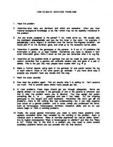
Fig. 1. The quantities involved in the shallow-water equations.

The shallow-water equations form a depth-integrated model for free surface flow of a fluid under the influence of gravity, see Figure 1. In the model, it is assumed that the height of the top surface above the bottom is sufficiently small compared with some characteristic length of motion. Moreover, vertical motion within the fluid is ignored, and we have hydrostatic balance in the vertical direction. For water waves over a bottom topography (bathymetry) B(x, y) in two spatial dimensions, this gives rise to the following inhomogeneous system         hu hv h 0  hu  +  hu2 + 1 gh2  +   =  −ghBx  . huv (7) 2 1 2 2 hv t −ghB gh huv hv + y 2 y x The right-hand side of (7) models the influence of a variable bathymetry. Figure 1 illustrates the situation and the quantities involved. The function B = B(x, y) describes the bathymetry, while w = B(x, y, t) models the water surface elevation, and we have that h = w − B. For brevity, we will refer to this system as Qt + F (Q)x + G(Q)y = H(Q, Z). The system has the following eigenvalues, λ(Q, n) = (u, v) · n ±

p gh, (u, v) · n

where a linear shear wave with characteristic wave-speed v has been introduced in addition to the two nonlinear waves described above. For simplicity, we will henceforth assume a flat bathymetry, for which H(Q, Z) ≡ 0. Example 6 contains a short discussion of variable bathymetry. 2.2 The Euler Equations Our second example of a hyperbolic system is given by the Euler equations for an ideal, polytropic gas. This system is probably the canonical example of

8


a hyperbolic system of conservation laws that describes conservation of mass, momentum (in each spatial direction) and energy. In one spatial dimension the equations read     ρ ρu Qt + F (Q)x =  ρu  +  ρu2 + p  = 0. (8) E t u(E + p) x and similarly in two dimensions       ρv ρu ρ 2      ρu     +  ρu + p  +  ρuv 2  ρv + p  = 0.  ρuv   ρv  v(E + p) y u(E + p) x E t

(9)

Here ρ denotes density, u and v velocity in x- and y- directions, p pressure, and E is the total energy (kinetic plus internal energy) given by E = 21 ρu2 + p/(γ − 1),

or

E = 21 ρ(u2 + v 2 ) + p/(γ − 1).

The gas constant γ depends on the species of the gas, and is, for instance, equal 1.4 for air. The eigenvalues of (8) are p λ(Q, n) = (u, v) · n ± γp/ρ, (u, v) · n, giving three waves: a slow nonlinear wave, a linear contact wave, and a fast nonlinear wave. In two space dimensions λ(Q, n) = (u, v) · n is a double eigenvalue corresponding both to a contact wave and a shear wave. A contact wave is characterised by a jump in density together with no change in pressure and velocity, i.e., ρ is discontinuous and p and (u, v) · n are constant, whereas a shear wave means a discontinuity in the tangential velocity (u, v) · n⊥ .

3 Two Classical Finite Volume Schemes A standard approach to numerical schemes for PDEs is to look for a pointwise approximation and replace temporal and spatial derivatives by finite differences. Alternatively, we can divide the domain Ω into a set of finite subdomains Ωi and then use the integral form of the equation to compute approximations to the cell average of Q over each grid cell Ωi . In one spatial dimension, the cell-average is given by Z xi+1/2 1 Qi (t) = Q(x, t) dx, (10) ∆xi xi−1/2 and similarly in two dimensions


Qi (t) =

1 |Ωi |

9

ZZ Q(x, y, t) dxdy.

(11)

Ωi

The corresponding schemes are called finite-volume schemes. To derive equations for the evolution of cell averages Qi (t) in one spatial dimension, we impose the conservation law on integral form (2) on the grid cell Ωi = [xi−1/2 , xi+1/2 ], which then reads Z d xi+1/2 Q(x, t) dx = F Q(xi−1/2 , t) − F Q(xi+1/2 , t) (12) dt xi−1/2 Using the integral form of the equation rather than the differential form is quite natural, as it ensures that also the discrete approximations satisfy a conservation property. From (12) we readily obtain a set of ordinary differential equations for the cell averages Qi (t), 1 d Qi (t) = − Fi+1/2 (t) − Fi−1/2 (t) , dt ∆xi where the fluxes across the cell-boundaries are given by Fi±1/2 (t) = F Q(xi±1/2 , t) .

(13)

(14)

To derive schemes for the two-dimensional shallow-water and Euler equations we will follow a similar approach. We will assume for simplicity that the finite volumes are given by the grid cells in a uniform Cartesian grid, such that Ωij = (x, y) ∈ (i − 1/2)∆x, (i + 1/2)∆x × (j − 1/2)∆y, (j + 1/2)∆y . To simplify the presentation, we henceforth assume that ∆x = ∆y. Then the semi-discrete approximation to (2) reads i d 1 h Qij (t) = Lij (Q(t)) = − Fi+1/2,j (t) − Fi−1/2,j (t) dt ∆x (15) i 1 h − Gi,j+1/2 (t) − Gi,j−1/2 (t) , ∆y where Fi±1/2,j and Gi,j±1/2 are numerical approximations to the fluxes over the cell edges Z yj+1/2 1 F Q(xi±1/2 , y, t) dy, Fi±1/2,j (t) ≈ ∆y yj−1/2 (16) Z xi+1/2 1 Gi,j±1/2 (t) ≈ G Q(x, yj±1/2 , t) dx. ∆x xi−1/2 Equation (15) is a set of ordinary differential equations (ODEs) for the timeevolution of the cell-average values Qij .

10


Modern high-resolution schemes are often derived using a finite-volume framework, as we will see in Section 4. To give the reader a gentle introduction to the concepts behind high-resolution schemes we start by deriving two classical schemes, the Lax–Friedrichs [28] and the Lax–Wendroff schemes [29], using the semi-discrete finite-volume framework. The exact same schemes can be derived using a finite-difference framework, but then the interpretation of the unknown discrete quantities would be different. The distinction between finite-difference and finite-volume schemes is not always clear in the literature, and many authors tend to use the term ‘finite-volume scheme’ to denote conservative schemes derived using finite differences. By conservative we mean a scheme that can be written on conservative form (in one spatial dimension): Qn+1 = Qni − r(Fi+1/2 − Fi−1/2 ), i

(17)

where Qni = Qi (n∆t) and r = ∆t/∆x. The importance of the conservative form was established through the famous Lax–Wendroff theorem [29], which states that if a sequence of approximations computed by a consistent and conservative numerical method converges to some limit, then this limit is a weak solution of the conservation law. To further motivate this form, we can integrate (12) from t to t+∆t giving Qi (t + ∆t) = Qi (t) Z Z t+1∆t i 1 h t+1∆t F (Q(xi+1/2 , t)) dt − F (Q(xi−1/2 , t)) dt . − ∆xi t t By summing (17) over all cells (for i = −M : N ) we find that the cell averages satisfy a discrete conservation principle N X i=−M

Qn+1 ∆x = i

N X

Qni ∆x − ∆t(FN +1/2 − F−M −1/2 )

i=−M

In other words, our discrete approximations P mimic the conservation principle of the unknown function Q since the sum i Qi ∆x approximates the integral of Q. 3.1 The Lax–Friedrichs Scheme We will now derive our first numerical scheme. For simplicity, let us first consider one spatial dimension only. We start by introducing a time-step ∆t and discretise the ODE (13) by the forward Euler method. Next, we must evaluate the flux-integrals (14) along the cell edges. We now make the assumption that Q(x, n∆t) is piecewise constant and equals the cell average Qni = Qi (n∆t) inside each grid cell. Then, since all perturbations in a hyperbolic system travel with a finite wave-speed, the problem of estimating the solution along the cell


11

edges can be recast as a set of locally defined initial-value problems on the form ( QL , x < 0, Qt + F (Q)x = 0, Q(x, 0) = (18) QR , x > 0. This is called a Riemann problem and is a fundamental building block in many high-resolution schemes. We will come back to the Riemann problem in Section 4.1. For now, we take a more simple approach to avoid solving the Riemann problem. For the Lax–Friedrichs scheme we approximate the flux function at each cell-boundary by the average of the fluxes evaluated immediately to the left and right of the boundary. Since we have assumed the function to be piecewise constant, this means that we will evaluate the flux using the cell averages in the adjacent cells, 1 F (Qni ) + F (Qni+1 ) , etc. F (Q(xi+1/2 , n∆t)) = 2 This approximation is commonly referred to as a centred approximation. Summing up, our first scheme reads i 1 h Qn+1 = Qni − r F Qni+1 − F Qni−1 . i 2 Unfortunately, this scheme is notoriously unstable. To obtain a stable scheme, we can add artificial diffusion (∆x2 /∆t)∂x2 Q. Notice, however, that by doing this, it is no longer possible to go back to the semi-discrete form, since the artificial diffusion terms blow up in the limit ∆t → 0. If we discretise the artificial diffusion term by a standard central difference, the new scheme reads 1 h i 1 n n n n Qn+1 = Q + Q − r F Q − F Q (19) i+1 i−1 i+1 i−1 . i 2 2 This is the classical first-order Lax–Friedrichs scheme. The scheme is stable provided the following condition is fulfilled r max |λF k (Qi )| ≤ 1, ik

(20)

where λF k are the eigenvalues of the Jacobian matrix of the flux function F . The condition is called the CFL condition and simply states that the domain of dependence for the exact solution, which is bounded by the characteristics of the smallest and largest eigenvalues, should be contained in the domain of dependence for the discrete equation. A two-dimensional scheme can be derived analogously. To approximate the integrals in (16) one can generally use any numerical quadrature rule. However, the midpoint rule is sufficient for the first-order Lax–Friedrichs scheme. Thus we need to know the point values Q(xi±1/2 , yj , n∆t) and Q(xi , yj±1/2 , n∆t). We assume that Q(x, y, n∆t) is piecewise constant and equal the cell average within each grid cell. The values of Q(x, y, n∆t) at the

12


midpoints of the edges can then be estimated by simple averaging of the onesided values, like in the one dimensional case. Altogether this gives the the following scheme 1 n n n n Q + Q + Q + Q Qn+1 = i+1,j i−1,j i,j+1 i,j−1 ij 4 i h i (21) 1 1 h − r F Qni+1,j − F Qni−1,j − r G Qni,j+1 − G Qni,j−1 , 2 2 which is stable under a CFL restriction of 1/2. The Lax–Friedrichs scheme is also commonly derived using finite differences as the spatial discretisation, in which case Qnij denotes the point values at (i∆x, j∆y, n∆t). The scheme is very robust. This is largely due to the added numerical dissipation, which tends to smear out discontinuities. A formal Taylor analysis of a single time step shows that the truncation error of the scheme is of order two in the discretisation parameters. Rather than truncation errors, we are interested in the error at a fixed time (using an increasing number of time steps), and must divide with ∆t, giving an error of order one. For smooth solutions the error measured in, e.g., the L∞ or L1 -norm therefore decreases linearly as the discretisation parameters are refined, and hence we call the scheme first-order. A more fundamental derivation of the Lax–Friedrichs scheme (21) is possible if one introduces a staggered grid (see Figure 9). To this end, let Qni+1 be the cell average over [xi , xi+2 , and Qn+1 be the cell average over the stagi gered cell [xi−1 , xi+1 ]. Then (19) is the exact evolution of the piecewise constant data from time tn to tn+1 followed by an averaging onto the staggered grid. This averaging introduces the additional diffusion discussed above. The two-dimensional scheme (21) can be derived analogously. 3.2 The Lax–Wendroff Scheme To achieve formal second-order accuracy, we replace the forward Euler method used for the integration of (13) by the midpoint method, that is, h i n+1/2 n+1/2 n Qn+1 = Q − r F − F (22) i i i+1/2 i−1/2 . n+1/2

To complete the scheme, we must specify the fluxes Fi±1/2 , which again depend on the values at the midpoints at time tn+1/2 = (n + 12 )∆t. One can show that these values can be predicted with acceptable accuracy using the Lax–Friedrichs scheme on a grid with grid-spacing 21 ∆x, n+1/2

Qi+1/2 =

1 h i 1 n n Qi+1 + Qni − r Fi+1 − Fin . 2 2

(23)

Altogether this gives a second-order, predictor-corrector scheme called the Lax–Wendroff scheme [29]. Like the Lax–Friedrichs scheme, the scheme in


13

(22)–(23) can be interpreted both as a finite difference and as a finite volume scheme, and the scheme is stable under a CFL condition of 1. For extensions of the Lax–Wendroff method to two spatial dimensions, see [42, 15, 32]. To get second-order accuracy, one must include cross-terms, meaning that the scheme uses nine points. A recent version of the two-dimensional Lax– Wendroff scheme is presented in [36]. We have now introduced two classical schemes, a first-order and a secondorder scheme. Before we describe how to implement these schemes on the GPU, we will illustrate their approximation qualities. Example 1. Consider a linear advection equation on the unit interval with periodic boundary data ut + ux = 0,

u(x, 0) = u0 (x),

u(0, t) = u(1, t).

As initial data u0 (x) we choose a combination of a smooth squared sine wave and a double step function, x − 0.1 π χ[0.1,0.4] (x) + χ[0.6,0.9] (x). u(x, 0) = sin2 0.3 Figure 2 shows approximate solutions after ten periods computed by Lax– Friedrichs and Lax–Wendroff on a grid with 100 cells for ∆t = 0.95∆x. Both schemes clearly give unacceptable resolution of the solution profile. The firstorder Lax–Friedrichs scheme smears both the smooth and the discontinuous part of the advected profile. The second-order Lax–Wendroff scheme preserves the smooth profile quite accurately, but introduces spurious oscillations at the two discontinuities. Consider next the nonlinear Burgers’ equation, ut + 21 u2 x = 0, u(x, 0) = u0 (x), u(0, t) = u(1.5, t), with the same initial data as above. Burgers’ equation can serve as a simple model for the nonlinear momentum equation in the shallow-water and the Euler equations. Figure 3 shows approximate solutions at time t = 1.0 computed by Lax–Friedrichs and Lax–Wendroff on a grid with 150 cells for ∆t = 0.95∆x. As in Figure 2, Lax–Friedrichs smooths the nonsmooth parts of the solution (the two shocks and the kink at x = 0.1), whereas Lax–Wendroff creates spurious oscillations at the two shocks. On the other hand, the overall approximation qualities of the schemes are now better due to self-sharpening mechanisms inherent in the nonlinear equation. To improve the resolution one can use a so-called composite scheme, as introduced by Liska and Wendroff [36]. This scheme is probably the simplest possible high-resolution scheme and consists of e.g., three steps of Lax– Wendroff followed by a smoothing Lax–Friedrichs step. The idea behind this scheme is that the numerical dissipation in the first-order Lax–Friedrichs scheme should dampen the spurious oscillations created by the second-order Lax–Wendroff scheme. In Figure 4 we have recomputed the results from Figures 2 and 3 using the composite scheme.

14

Hagen, Henriksen, Hjelmervik, and Lie Lax–Friedrichs’ method

Lax–Wendroff’s method

1

1

0.8

0.8

0.6

0.6

0.4

0.4

0.2

0.2

0

0

−0.2

−0.2

0

0.1

0.2

0.3

0.4

0.5

0.6

0.7

0.8

0.9

1

0

0.1

0.2

0.3

0.4

0.5

0.6

0.7

0.8

0.9

1

Fig. 2. Approximate solutions at time t = 10.0 for the linear advection equation computed by the Lax–Friedrichs and the Lax–Wendroff schemes. Lax–Friedrichs’ method

Lax–Wendroff’s method

0.8

0.8

0.7

0.7

0.6

0.6

0.5

0.5

0.4

0.4

0.3

0.3

0.2

0.2

0.1

0.1

0

0 0

0.5

1

1.5

0

0.5

1

1.5

Fig. 3. Approximate solutions at time t = 1.0 for Burgers’ equation. composite method

composite method 0.8

1

0.7

0.6

0.8

0.5 0.6

0.4 0.4

0.3 0.2

0.2

0.1

0

0 −0.2

0

0.1

0.2

0.3

0.4

0.5

0.6

0.7

0.8

0.9

1

0

0.5

1

1.5

Fig. 4. Approximate solution at time t = 10.0 for the linear advection equation (left) and at time t = 1.0 for Burgers’ equation (right) computed by a composite scheme.


15

The previous example demonstrated the potential shortcomings of classical schemes, and such schemes are seldomly used in practice. On the other hand, they have a fairly simple structure and are therefore ideal starting points for discussing how to implement numerical methods on the GPU. In the next subsection, we therefore describe how to implement the Lax–Friedrichs scheme on the GPU. 3.3 Implementation on the GPU Before we start discussing the actual implementation the Lax–Friedrichs scheme, let us look briefly into the design of a graphics card and its associated programming model. GPUs operate in a way that is similar to a shared-memory parallel computer of the single-instruction-multiple-data (SIMD) type. In a SIMD computer, a single control unit dispatches instructions to a large number of processing nodes, and each node executes the same instruction on its own local data. SIMD computers are obviously particularly efficient when the same set of operations can be applied to all data items. If the execution involves conditional branches, there may be a performance loss since processing nodes in the worst case must execute both branches and thereafter pick the correct result. In a certain sense, explicit high-resolution schemes are good candidates for a SIMD implementation, since the update of each grid-cell involves a fixed set of given arithmetic operations and seldom introduces conditional branches in the instruction stream. Let us now look at how computations are dispatched in a GPU. The main objective of the GPU is to render geometrical primitives (points, lines, triangles, quads), possibly combined with one or more textures (image data), as discrete pixels in a frame buffer (screen or off-screen buffer). When a primitive is rendered, the rasterizer samples the primitive at points corresponding to the pixels in the frame buffer. Per vertex attributes such as texture coordinates are set by the application for each vertex and the rasterizer calculates an interpolated value of these attributes for each point. These bundles of values then contain all the information necessary for calculating the color of each point, and are called fragments. The processing pipeline is illustrated in Figure 5. We see that whereas a CPU is instruction-driven, the programming model of a GPU is data-driven. This means that individual data elements of the data-stream can be pre-fetched from memory before they are processed, thus avoiding the memory latency that tends to hamper CPUs. Graphics pipelines contain two programmable parts, the vertex processor and the fragment processor. The vertex processor operates on each vertex (corner of a primitive) without knowledge of surrounding vertices or the primitive to which it belongs. The fragment processor works in the same manner, it operates on each fragment in isolation. Both processors use several parallel pipelines, and thus work on several vertices/fragments simultaneously. To implement our numerical schemes (or a graphical algorithm) we must specify the

16


geometric primitives (lines,triangles,..)

Vertex processor (programmable)

vertex data (xyzw)

Rasterizer

fragments Fragment processor fragments (programmable)

Frame buffer (2D set of pixels)

Texture (rgba image) rgba values Texture (rgba image)

Fig. 5. A schematic of the graphics pipeline.

operations in the vertex and fragment processors. To this end, we make one or more shaders; these are codes written in a high-level, often C-like, language like Cg or Open GL Shading Language (GLSL), and are read and compiled by our graphical application into programs that are run by the vertex and fragment processors. Consult the references [14] and [43] for descriptions of these languages. The compiled shaders are executed for each vertex/fragment in parallel. Our data model will be as follows: The computational domain is represented as an off-screen buffer. A geometric primitive is rendered such that a set of Nx × Ny fragments is generated which covers the entire domain. In this model, we never explicitly loop over all cells in the grid. Instead, processing of each single grid-cell is invoked implicitly by the rasteriser, which interpolates between the vertices and generates individual data for each fragment. Input field-values are realised in terms of 2D textures of size Nx × Ny . Between iterations, the off-screen buffer is converted into a texture, and another off-screen buffer is used as computational domain. To solve the conservation law (3), the fragment processor loads the necessary data and performs the update of cell averages, according to (21) for the Lax–Friedrichs scheme. In this setting, the vertex processor is only used to set texture coordinates that are subsequently passed to the fragment processor. The fragment processor is then able to load the data associated with the current cell and its neighbours from the texture memory. In the following subsection we will discuss the implementation of fragment shaders in detail for the Lax–Friedrichs scheme. However, to start the computations, it is necessary to set up the data stream to be processed and to configure the graphics pipeline. This is done in a program running on the CPU. Writing such a program requires a certain familiarity with the graphics processing jargon, and we do not go into this issue—the interested reader is referred to [44, 13, 41]. Shaders for Lax–Friedrichs Listing 1 shows the vertex and fragment shader needed to run the Lax– Friedrichs scheme (21) for the two-dimensional shallow-water equations (7) with constant bottom topography B ≡ 0. In the listing, all entities given in


17

Listing 1. Fragment and vertex shader for the Lax–Friedrichs scheme written in GLSL. [Vertex shader] varying vec4 texXcoord; varying vec4 texYcoord; uniform vec2 dXY; void main(void) { texXcoord=gl MultiTexCoord0.yxxx+vec4(0.0,0.0,−1.0,1.0)∗dXY.x; texYcoord=gl MultiTexCoord0.xyyy+vec4(0.0,0.0,−1.0,1.0)∗dXY.y;

// j , i , i−1, j+1 // i , j , j−1, j+1

gl Position = gl ModelViewProjectionMatrix ∗ gl Vertex; }

[Fragment shader] varying vec4 texXcoord; varying vec4 texYcoord; uniform sampler2D QTex; uniform float r; uniform float halfG; vec4 fflux(in vec4 Q) { float u=Q.y/Q.x; return vec4( Q.y, (Q.y∗u + halfG∗Q.x∗Q.x), Q.z∗u, 0.0 ); } vec4 gflux(in vec4 Q) { float v=Q.z/Q.x; return vec4( Q.z, Q.y∗v, (Q.z∗v + halfG∗Q.x∗Q.x), 0.0 ); } void main(void) { vec4 QE = texture2D(QTex, texXcoord.wx); vec4 QW = texture2D(QTex, texXcoord.zx); vec4 QN = texture2D(QTex, texYcoord.xw); vec4 QS = texture2D(QTex, texYcoord.xz); gl FragColor = 0.25∗(QE + QW + QN + QS) − 0.5∗r∗(fflux (QE) − fflux(QW)) − 0.5∗r∗(gflux(QN) − gflux(QS)); }

boldface are keywords and all entities starting with gl_ are built-in variables, constants, or attributes. The vertex shader is executed once for all vertices in the geometry. Originally, the geometry is defined in a local coordinate system called object-space or model coordinates. The last line of the vertex shader transforms the vertices from object-space to the coordinate system of the camera (view coordinates, or eye-space). The two coordinate systems will generally be different. Dur-

18


ing the rendering phase only points inside the camera view (i.e., inside our computational domain) are rendered. In the shader, the model coordinates are given by gl_Vertex and the projected view coordinates are returned by gl_Position. The coordinate transformation is an affine transformation given by a global matrix called gl_ModelViewProjectionMatrix. (Since the camera does not move, this transformation is strictly speaking not necessary to perform for every time step and could have been done once and for all on the CPU). The first two lines of the vertex shader compute the texture coordinates. These coordinates will be used by the fragment shader to fetch values in the current cell and its four nearest neighbours from one or more texture. The keywords vec2 and vec4 declares vector variables with 2 or 4 elements respectively. The construction varying vec4 texXcoord means that the fourcomponent vector texXcoord will be passed from the vertex shader to the fragment shader. This happens as follows: The vertex shader defines one vector-value V at each vertex (the four corners of our computational rectangle), and the rasteriser then interpolates bilinearly between these values to define corresponding values for all fragments within the camera view. In contrast, uniform vec2 dXY means that dXY is constant for each primitive; its value must be set by the application program running on the CPU. Notice how we can access individual members of a vector as V.x, V.y, V.z and V.w, or several elements e.g., V.xy or V.wzyx. The last example demonstrates ‘swizzling’; permuting the components of the vector. We now move on to the fragment shader. Here we see the definitions of the texture coordinates texXcoord and texYcoord, used to pass coordinates from the vertex processor. UTex is a texture handle; think of it as a pointer to an array. The constants r and halfG represent r = ∆t/∆x and 12 g, respectively. To fetch the cell-averages from positions in the texture corresponding to the neighbouring cells, we use the function texture2D. The new cell-average is returned as the final fragment colour by writing to the variable gl_FragColor. To ensure a stable scheme, we must ensure that the time step satisfies a CFL condition of the form (20). This means that we have to gather the eigenvalues from all points in the grid to determine the maximum absolute value. In parallel computing, such a gather operation is usually quite expensive and represents a bottleneck in the processing. By rethinking the gather problem as a graphics problem, we can actually use hardware supported operations on the GPU to determine the maximal characteristic speed. Recall that the characteristic speed of each wave is given by the corresponding eigenvalue. To this end we pick a suitably sized array, say 16 × 16, and decompose the computational domain Nx × Ny into rectangular subdomains (quads) so that each subdomain is associated with a 16 × 16 patch of the texture containing the Q-values. All quads are moved so that they coincide in world-coordinates, and hence we get Nx Ny /162 overlapping quads. By running the fragment shader in Listing 2 they are rendered to the depth buffer. The purpose of the depth buffer is to determine whether a pixel is behind or in front of another. When a


19

Listing 2. Fragment shader written in GLSL for determining the maximum characteristic speed using the depth buffer. uniform sampler2D QnTex; uniform float scale; uniform float G; void main(void) { vec4 Q = texture2D(QnTex, gl TexCoord[0].xy); Q.yz /= Q.x; float c = sqrt( G∗Q.x ); float r = max(abs(Q.y) + c, abs(texQ.z) + c); r ∗= scale ; gl FragDepth = r; }

fragment is rendered to the depth buffer, its depth value is therefore compared with the depth value that has already been stored for the current position, and the maximum value is stored. This process is called depth test. In our setting this means that when all quads have been rendered, we have a 16 × 16 depth buffer, where each value represents the maximum over Nx Ny /162 values. The content of the 16 × 16 depth buffer is read back to the CPU, and the global maximum is determined. Since the depth test only accepts values in the interval [0, 1], we include an appropriate scaling parameter scale passed in from the CPU. 3.4 Boundary Conditions In our discussions above we have tacitly assumed that every grid cell is surrounded by neighbouring cells. In practise, however, all computations are performed on some bounded domain and one therefore needs to specify boundary conditions. On a CPU, an easy way to impose boundary conditions is to use ghost cells; that is, to extend the domain by extra grid cells along the boundaries, whose values are set at the beginning of each time step (in the ODE solver). See [32] for a thorough discussion of different boundary conditions and their implementation in terms of ghost cells. There are many types of boundary conditions: Outflow (or absorbing) boundary conditions simply let waves pass out of the domain without creating any reflections. The simplest approach is to extrapolate grid values from inside the domain in each spatial direction. Reflective boundary conditions are used to model walls or to reduce computational domains by symmetry. They are realised by extrapolating grid values from inside the domain in each spatial direction and reversing the sign of the velocity component normal to the boundary. Periodic boundary conditions are realised by copying values from grid cells inside the domain at the opposite boundary.

20


Inflow boundary conditions are used to model a given flow into the domain through certain parts of the boundary. These conditions are are generally more difficult to implement. However, there are many cases for which inflow can be modelled by assigning fixed values to the ghost cells. In this paper we will only work with outflow boundary conditions on rectangular domains. The simplest approach is to use a zeroth order extrapolation, which means that all ghost cells are assigned the value of the closest point inside the domain. Then outflow boundaries can be realised on the GPU simply by specifying that our textures are clamped, which means that whenever we try to access a value outside the domain, a value from the boundary is used. For higher-order extrapolation, we generally need to introduce an extra rendering pass using special shaders that render the correct ghost-cell values to extended textures. 3.5 Comparison of GPU versus CPU We will now present a few numerical examples that compare the efficiency of our GPU implementation with a straightforward single-threaded CPU implementation of the Lax–Friedrichs scheme. The CPU simulations were run on a Dell Precision 670 which is a EM64T architecture with a dual Intel Xeon 2.8 GHz processor with 2.0 GB memory running Linux (Fedora Core 2). The programs were written in C and compiled using icc -O3 -ipo -xP (version 8.1). The GPU simulations were performed on two graphics cards from consecutive generations of the nVidia GeForce series: (i) the GeForce 6800 Ultra card released in April 2004 with the nVidia Forceware version 71.80 beta drivers, and (ii) the GeForce 7800 GTX card released in June 2005 with the nVidia Forceware version 77.72 drivers. The GeForce 6800 Ultra has 16 parallell pipelines, each capable of processing vectors of length 4 simultaneously. On the GeForce 7800 GTX, the number of pipelines is increased to 24. In the following we will for simplicity make comparisons on N × N grids, but this is no prerequisite for the GPU implementation. Rectangular N × M grids work equally well. Althought the current capabilities of our GPUs allow for problems with sizes up to 4096 × 4096, we have limited the size of our problems to 1024 × 1024 (due to high computational times on the CPU). Example 2 (Circular dambreak). Let us first consider a simple dambreak problem with rotational symmetry for the shallow-water equations; that is, we consider two constant states separated by a circle ( p x2 + y 2 ≤ 0.3, 1.0, h(x, y, 0) = 0.1, otherwise, u(x, y, 0) = v(x, y, 0) = 0. We assume absorbing boundary conditions. The solution consists of an expanding circular shock wave. Within the shock there is a rarefaction wave


21

0.5

0.4

0.3

0.2

0.1

0

0

0.1

0.2

0.3

0.4

0.5

0.6

0.7

0.8

0.9

1

Fig. 6. Scatter plot of the circular dambreak problem at t = 0.5 computed by Lax–Friedrichs scheme on a 128 × 128 grid. The dashed line is a fine-grid reference solution.

transporting water from the original deep region out to the shock. In the numerical computations the domain is [−1.0, 1.0] × [−1.0, 1.0] with absorbing boundary conditions. A reference solution can be obtained by solving the reduced inhomogeneous system 1 hur hu h + =− , hur t hu2r + 21 gh2 r r hu2r √ in which ur = u2 + v 2 denotes the radial velocity. This system is nothing but the one-dimensional shallow-water equations (5) with a geometric source term. Figure 6 shows a scatter plot of the water height at time t = 0.5 computed by the Lax–Friedrichs. In the scatter plot, the cell averages of a given quantity in all cells are plotted against the radial distance from the origin to the cell centre. Scatter plots are especially suited for illustrating grid-orientation effects for radially symmetric problems. If the approximate solution has perfect symmetry, the scatter plot will appear as a single line, whereas any symmetry deviations will show up as point clouds. The first-order Lax–Friedrichs scheme clearly smears both the leading shock and the tail of the imploding rarefaction wave. This behaviour is similar to what we observed previously in Figures 2 and 3 in Example 1 for the linear advection equation and the nonlinear Burgers’ equation. Table 1 reports a comparison of average runtime per time step for GPU versus CPU implementations of the Lax–Friedrichs scheme. Here, however, we see a that the 7800 GTX card with 24 pipelines is about two to three times faster than the 6800 Ultra card with 16 pipelines. The reason is as follows: For the simple Lax–Friedrichs scheme, the number of (arithmetic) operations performed per fragment in each rendering pass (i.e., the number of operations per grid point) is quite low compared with the number of texture fetches. We therefore cannot expect to fully utilize the computational potential of the GPU. In particular for the 128 × 128 grid, the total number of fragments

22


Table 1. Runtime per time step in seconds and speedup factor for the CPU versus the GPU implementation of Lax–Friedrichs scheme for the circular dambreak problem run on a grid with N × N grid cells, for the nVidia GeForce 6800 Ultra and GeForce 7800 GTX graphics cards. N

CPU

6800

speedup

7800

speedup

128 256 512 1024

2.22e-3 9.09e-3 3.71e-2 1.48e-1

7.68e-4 1.24e-3 3.82e-3 1.55e-2

2.9 7.3 9.7 9.5

2.33e-4 4.59e-4 1.47e-3 5.54e-3

9.5 19.8 25.2 26.7

Table 2. Runtime per time step in seconds and speedup factor for the CPU versus the GPU implementation of Lax–Friedrichs for the shock-bubble problem run on a grid with N × N grid cells, for the nVidia GeForce 6800 Ultra and GeForce 7800 GTX graphics cards. N

CPU

6800

speedup

7800

speedup

128 256 512 1024

3.11e-3 1.23e-2 4.93e-2 2.02e-1

7.46e-4 1.33e-3 4.19e-3 1.69e-2

4.2 9.3 11.8 12.0

2.50e-4 5.56e-4 1.81e-3 6.77e-3

12.4 22.1 27.2 29.8

processed per rendering pass on the GPU is low compared with the costs of switching between different rendering buffers and establishing each pipeline. The cost of these context switches will therefore dominate the runtime on the 6800 Ultra card, resulting in a very modest speedup of about 3–4. For the 7800 GTX, the cost of context switches is greatly reduced due to improvments in hardware and/or drivers, thereby giving a much higher speedup factor. Example 3 (Shock-bubble interaction). In this example we consider the interaction of a planar shock in air with a circular region of low density. The setup is as follows (see Figure 7): A circle with radius 0.2 is centred at (0.4, 0.5). The gas is initially at rest and has unit density and pressure. Inside the circle the density is 0.1. The incoming shock wave starts at x = 0 and propagates in the positive x-direction. The pressure behind the shock is 10, giving a 2.95 Mach shock. The domain is [0, 1.6]×[0, 1] with symmetry about the x axis. Figure 7 shows the development of the shock-bubble interaction in terms of (emulated) schlieren images. Schlieren imaging is a photo-optical technique for studying the distribution of density gradients within a transparent medium. Here we have imitated this technique by depicting (1 − |∇ρ|/ max |∇ρ|)p for p = 15 as a greymap. Figure 8 shows the result of a grid refinement study for Lax–Friedrichs. Whereas the scheme captures the leading shock on all grids, the weaker waves in the deformed bubble are only resolved satisfactorily on the two finest grids.


t=0.0

t=0.1

t=0.2

t=0.3

23

Fig. 7. Emulated schlieren images of a shock-bubble interaction. The approximate solution is computed by the composite scheme [36] on a 1280 × 800 grid.

Fig. 8. Grid refinement study of the shock-bubble case at time t = 0.3 computed with the Lax–Friedrichs scheme for ∆x = ∆y = 1/100, 1/200, 1/400, and 1/800.

24


To study the efficiency of a GPU implementation versus a CPU implementation of the Lax–Friedrichs scheme, we reduced the computational domain to [0, 1] × [0, 1] and the final simulation time to t = 0.2. Runtime per time step and speedup factors are reported in Table 2. Comparing with the circular dambreak case in Table 1, we now observe that whereas the runtime per time step on the CPU increases by a factor between 1.3–1.4, the runtime on the GPU increases at most by a factor 1.1. The resulting increase in speedup factor is thus slightly less than 4/3. This can be explained as follows: Since the shallow-water equations have only three components, the GPU only exploits 3/4 of its processing capabilities in each vector operation, whereas the Euler equations have four component and can exploit the full vector processing capability. However, since the flux evaluation for the Euler equations is a bit more costly in terms of vector operations, and since not all operations in the shaders are vector operations of length four, the increase in speedup factor is expected to be slightly less than 4/3. 3.6 Floating Point Precision When implementing PDE solvers on the CPU it is customary to use double precision. The current generations of GPUs, however, are only able to perform floating point operations in single precision (32 bits). The single precision numbers of the GPU have the format ‘s23e8’, i.e., there are 6 decimals in the mantissa. As a result, the positive range of representable numbers is [1.175 · 10−38 , 3.403 · 1038 ], and the smallest number s , such that 1 + s − 1 > 0, is 1.192 · 10−7 . Since the movie industry uses double precision (64 bits) in parts of the rendering system this also may become available in GPUs in the near future. The double precision numbers of our CPU have the format ‘s52e11’, i.e., mantissa of 15 decimals, range of [2.225 · 10−308 , 1.798 · 10308 ], and d = 2.220 · 10−16 . Ideally, the comparison between the CPU and the GPUs should have been performed using the same precision. Since CPUs offer single precision, this may seem to be an obvious choice. However, on current CPUs, double precision is supported in hardware, whereas single precision is emulated. This means that computations in single precision may be slower the computations in double precision on a CPU. We therefore decided not to use single precision on the CPU. The question is now if using single precision will effect the quality of the computed result. For the cases considered herein, we have computed all results on the CPU using both double and single precision. In all cases, the maximum difference of any cell average is of the same order as s . Our conclusion based on these quantitative studies is that the GPU’s lack of double precision does not deteriorate the computations for the examples considered in Sections 3.5 and 5. Please note that the methods considered in this paper are stable, meaning they cannot break down due to rounding errors.


25

4 High-Resolution Schemes Classical finite difference schemes rely on the computation of point values. In the previous section we saw how discontinuities lead to problems like oscillations or excessive smearing for two basic schemes of this type. For pedagogical reasons we presented the derivation of the two schemes in a semi-discrete, finite-volume setting, but this does not affect (in)abilities of the schemes in the presence of discontinuities. Modern high-resolution schemes of the Godunov type aim at delivering high-order resolution of all parts of the solution, and in particular avoiding the creation of spurious oscillations at discontinuities. There are several approaches to high-resolution schemes. Composite schemes form one such approach, see [36]. In the next sections we will present another approach based on geometric considerations. 4.1 The REA Algorithm Let us now recapitulate how we constructed our approximate schemes in Section 3. If we abstract our approach, it can be seen to consist of three basic parts: 1. Starting from the known cell-averages Qnij in each grid cell, we reconstruct b y, tn ) defined for all (x, y). For a a piecewise polynomial function Q(x, n b first-order scheme, we let Q(x, y, t ) be constant over each cell, i.e., b y, tn ) = Qn , Q(x, ij

(x, y) ∈ [xi−1/2 , xi+1/2 ] × [yj−1/2 , yj+1/2 ].

In a second-order scheme we use a piecewise bilinear reconstruction, and in a third order scheme a piecewise quadratic reconstruction, and so on. The purpose of this reconstruction is to go from the discrete set of cellaverages we use to represent the unknown solution and back to a globally defined function that is to be evolved in time. In these reconstructions special care must be taken to avoid introducing spurious oscillations into the approximation, as is done by classical higher-order schemes like e.g., Lax–Wendroff. 2. In the next step we evolve the differential equation, exactly or approxib y, tn ) as initial data. mately, using the reconstructed function Q(x, b y, tn+1 ) onto the grid again 3. Finally, we average the evolved solution Q(x, to give a new representation of the solution at time tn+1 in terms of cell averages Qn+1 ij . This three-step algorithm is often referred to as the REA algorithm, from the words reconstruct-evolve-average. The Riemann Problem To evolve and average the solution in Steps 2 and 3 of the REA algorithm, we generally use a semi-discrete evolution equation like (15). We thus need

26


to know the fluxes out of each finite-volume cell. In Section 3.1 we saw how the problem of evaluating the flux over the cell boundaries in one spatial dimension could be recast to solve a set of local Riemann problems of the form ( QL , x < 0, Qt + F (Q)x = 0, Q(x, 0) = QR , x > 0. The Riemann problem has a similarity solution of the form Q(x, t) = V (x/t). The similarity solution consists of constant states separated by simple waves that are either continuous (rarefactions) or discontinuous (shocks, contacts, shear waves, etc) and is therefore often referred to as the Riemann fan. Thus, to compute the flux over the cell edge, all we need to know is V (0). However, obtaining either the value V (0) or a good approximation generally requires detailed knowledge of the underlying hyperbolic system. The algorithm used to compute V (0) is called a Riemann solver. Riemann solvers come in a lot of flavours. Complete solvers, whether they are exact or approximate, use detailed knowledge of the wave structure and are able to resolve all features in the Riemann fan. Exact Riemann solvers are available for many systems, including the Euler and the shallow-water equations, but are seldomly used in practice since they tend to be relatively complicated and expensive to compute. Incomplete solvers, like the central-upwind or HLL solver presented in Section 4.5, lump all intermediate waves and only resolve the leading waves in the Riemann fan, thereby giving only a rough estimate of the centre state. A significant amount of the research on high-resolution schemes has therefore been devoted to developing (approximate) numerical Riemann solvers that are fast and accurate. The Riemann problem is thoroughly discussed in the literature, the interested reader might start with [30] and then move on to [48, 49] for a thorough discussion of different Riemann solvers for the Euler and the shallow-water equations. 4.2 Upwind and Centred Godunov Schemes The REA algorithm above is a general approach for constructing the so-called Godunov schemes that have ruled the ground in conservation laws during the last decades. Godunov schemes generally come in two flavors: upwind or centred schemes. To illustrate their difference, we will make a slight detour into fully discrete schemes. For simplicity, we consider only the one-dimensional scalar case. Instead of the cell average (10) we introduce a sliding average ¯ t) = 1 Q(x, ∆x

Z

x+∆x/2

Q(ξ, t) dξ. x−∆x/2

Analogously to (13), we can derive an evolution equation for the sliding average


xi−1/2

xi−1/2

xi+1/2

xi

xi+1/2

27

xi+3/2

xi+1

xi+3/2

Fig. 9. Sliding average for upwind schemes (top) and centred schemes (bottom). The dashed boxes show the integration volume in the (x, t) plane. The shaded triangles and solid lines emanating from xi−1/2 , xi+1/2 and xi+3/2 illustrate the self-similar Riemann fans, whereas the dashed lines indicate the cell edges at time tn .

¯ t + ∆t) = Q(x, ¯ t) Q(x, Z t+∆t 1 − F Q(x + ∆x t

∆x 2 , τ)

− F Q(x −

∆x 2 , τ)

dτ. (24)

Within this setting, we obtain an upwind scheme if we choose x = xi in (24) and a centred scheme for x = xi+1/2 . Figure 9 illustrates the fundamental difference between these two approaches. In the upwind scheme, the flux is integrated over the points xi±1/2 , where the reconstruction is generally discontinuous. To integrate along the cell interface in time we will therefore generally have to find the self-similar solution of the corresponding Riemann problem (18) along the space-time ray (x − xi±1/2 )/t = 0. To this end, one uses either exact or approximate Riemann solvers, as discussed above. Centred schemes, on the other hand, use a sliding average defined over a staggered grid cell [xi , xi+1 ], cf. the dashed box in the lower half of Figure 9. Thus the flux is integrated at the points xi and xi+1 , where the solution is continuous if ∆t satisfies a CFL condition of 1/2. This means that no explicit wave propagation information for the Riemann fans is required to integrate the flux, since in this case the Riemann fan is inside confinement of the associated staggered cells. Since they use less information about the specific conservation law being solved, centred schemes tend to be less accurate than upwind schemes. On the other hand, they are much simpler to implement and work pretty well as black-box solvers.

28


The first staggered high-resolution scheme based upon central differences was introduced by Nessyahu and Tadmor [39], who extended the staggered Lax–Friedrichs scheme (19) discussed in Section 3.1 to second order. Similarly, the scheme has later been extended to higher order and higher dimensions by e.g., Arminjon et al. [3], Russo et al. [7, 33], and Tadmor et al [37, 22]. Joint with S. Noelle, the fourth author (Lie) has contributed to the research on staggered schemes, see [34, 35]. A complete overview of staggered highresolution methods is outside the scope of the current presentation, instead we refer the reader to Tadmor’s Central Station http://www.cscamm.umd.edu/~tadmor/centralstation/ which has links to virtually all papers written on high-resolution central schemes, and in particular, on staggered schemes. Non-staggered centred schemes can be obtained if the new solution at time t + ∆t is first reconstructed over the staggered cell and then averaged over the original cell to define a new cell-average at time t + ∆t. In certain cases, semi-discrete schemes can then be obtained in the limit ∆t → 0. We do not present derivations here; the interested reader is referred to e.g., [25, 24]. 4.3 Semi-Discrete High-Resolution Schemes Let us now return to the semi-discretised equation (15). Before we can use this equation for computing, we must answer two questions: how do we solve the ODEs evolving the cell-average values Qij , and how do we compute the edge fluxes (16)? The ODEs are usually solved by an explicit predictor-corrector scheme of Runge–Kutta type. In each substep of the Runge–Kutta method the right-hand side of (15) is computed by evaluating the flux integrals according to some standard quadrature rule. To apply a quadrature rule, two more points need to be clarified: how to compute point-values of Q from the cell-averages, and how to evaluate the integrand of the edge fluxes at the integration points. Listing 3 shows a general algorithm based on (15). Different schemes are distinguished by the three following points: the reconstruction used to compute point-values, the discretisation and evaluation of flux integrals, and the ODE-solver for (15). In the following we will describe all these parts in more detail. We start with the ODE-solver, move on to the flux evaluation, and in the next section consider the reconstruction. We return to the flux evaluation in Section 4.5. Runge–Kutta ODE Solver To retain high-order accuracy in time without creating spurious oscillations, it is customary to use so-called TVD Runge–Kutta methods [45] as the ODEsolver. These methods employ a convex combination of forward Euler steps to advance the solution in time. They are especially designed to maintain the


29

Listing 3. General algorithmic form of a semi-discrete, high-resolution scheme, written in quasi-C code Q[N RK]=make initial data(); // Main loop for (t=0; t 0,   b, if |b| < |a| and ab > 0, which picks the least slope and reduces to zero at extrema in the data. For systems of conservation laws, solution are not necessarily bounded in supnorm or have diminishing total variation. Still, it is customary to apply the same design principle as for scalar equations. In our experiments, we have also used the modified minmod limiter and the superbee limiter  0, if ab ≤ 0,    θa, if (2θ − 1)ab < b2 , MMθ (a, b) = 1 2    2 (a + b), if ab < (2θ − 1)b ,  θb, otherwise,   0, if ab ≤ 0,      θa, if θab < b2 ,  SBθ (a, b) = b, if ab < b2 ,    a, if ab < θb2    θb, otherwise. Away from extrema, the minmod always chooses the one-sided slope with least magnitude, whereas the other two limiters tend to choose steeper reconstruction, thus adding less numerical viscosity into the scheme. For other families of limiter, see e.g., [35, 48]. Listing 5 shows the fragment shader implementing the bilinear reconstruction. This shader needs to return two vectors corresponding to ∆x∂x Q and ∆y∂y Q. At the time of implementation, GLSL was not capable of simultaneously writing to two textures due to problems with our drivers, we therefore chose to implemented the shader in Cg using so-called multiple render targets. In our implementation, we write to two textures using the new structure


33

Listing 5. Fragment shader in Cg for the bilinear reconstruction float4 minmod(in float4 a, in float4 b) { float4 res = min(abs(a), abs(b)); return res∗(sign(a)+sign(b))∗0.5; }

// minmod function

struct f2b { float4 color0 float4 color1 };

// Return two fragment buffers // d x Q // d y Q

: COLOR; : COLOR1;

struct v2f input { float4 pos : POSITION; float4 texXcoord; float4 texYcoord; };

// // // //

Current stencil Position Offsets in x Offsets in y

f2b main(v2f input IN, uniform sampler2D QnTex, uniform float2 dXYf) { f2b OUT; Q {ij} Q {i+1,j} Q {i−1,j} d x Q {ij}

float4 Q = tex2D(QnTex, IN.texXcoord.yx); float4 QE = tex2D(QnTex, IN.texXcoord.wx); float4 QW = tex2D(QnTex, IN.texXcoord.zx); OUT.color0 = minmod(Q−QW, QE−Q);

// // // //

float4 QN = tex2D(QnTex, IN.texYcoord.xw); float4 QS = tex2D(QnTex, IN.texYcoord.xz); OUT.color1 = minmod(Q−QS, QN−Q);

// Q {i,j+1} // Q {i,j−1} // d y Q {ij}

return OUT; }

f2b. Moreover, to avoid introducing conditional branches that can reduce the computational efficiency, we have used the non-conditional version (31) rather than the conditional version (32) of the minmod-limiter. Higher-order accuracy can be obtained by choosing a higher-order reconstruction. Two higher-order reconstructions are presented in Appendix A; the CWENO reconstruction in Appendix A.1 is a truly multidimensional reconstruction giving third order spatial accuracy, whereas the dimension-bydimension WENO reconstruction in Appendix A.2 is designed to give fifth order accuracy at Gaussian integration points. 4.5 Numerical Flux In the previous section we presented a reconstruction approach for obtaining one-sided point values at the integration points of the flux quadrature (28). All that now remains to define a fully discrete scheme is to describe how to use these point-values to evaluate the integrand itself. In the following we will introduce a few fluxes that can be used in combination with our highresolution semi-discrete schemes.

34


Centred Fluxes In Sections 3.1 and 3.2 we introduced two classical centred fluxes, the Lax– Friedrichs flux: F LF =

1 ∆x 1 F QL + F QR − QR − QL , 2 2 ∆t

and the Lax–Wendroff flux F LW = F Q∗ , 1 ∆t 1 Q∗ = QL + QR − F QR − F QL . 2 2 ∆x By taking the arithmetic average of these two fluxes, one obtains the FORCE flux introduced by Toro [48] F F ORCE =

1 ∆x 1 F QL + 2F Q∗ + F QR − QR − QL , 4 4 ∆t

(33)

In the above formulae QL and QR denote the point values extrapolated from left and right at the Gaussian integration points. If used directly with the cell averaged values (and with forward Euler as time integrator), the FORCE flux gives an oscillatory second-order method. A Central-Upwind Flux So far, wave propagation information has only been used to ensure stability through a CFL condition. Let us now incorporate information about the largest and smallest eigenvalues into the flux evaluation, while retaining the centred approach. This will lead to so-called central-upwind fluxes, as introduced by Kurganov, Noelle, and Petrova [24]. To this end, we define a+ = max λm Q , 0 , Q∈{QL ,QR } − a = min λ1 Q , 0 , Q∈{QL ,QR }

where λ1 is the smallest and λm the largest eigenvalues of the Jacobian matrix of the flux F . If the system is not genuinely nonlinear or linearly degenerate, the minimum and maximum is taken over the curve in phase space that connects QL and QR . The values (a− , a+ ) are estimates of how far the Riemann fan resulting from the discontinuity (QL , QR ) extends in the negative and positive direction. Using this information, the evolving solution can be divided into two unions of local sets: one covering the local Riemann fans, where the solution is possibly discontinuous and one covering the area in-between, where the solution is smooth, see Figure 10. By evolving and averaging separately in the two sets, the following flux function can be derived [24]


xi−1

xi−1/2

xi

xi+1/2

xi+1

xi+3/2

35

xi+2

Fig. 10. Spatial averaging in the REA algorithm for the central-upwind scheme.

F

CU W

a+ F QL − a− F QR a+ a− + + QR − QL . = + − − a −a a −a

(34)

The name “central-upwind” comes from the fact that for monotone flux functions, the flux reduces to the standard upwind method. For example, for scalar equations with F 0 (Q) ≥ 0, a− is zero and F CU W = F (QL ). Moreover, the first-order version of the scheme (i.e., for which QL = Qi and QR = Qi+1 ) is the semi-discrete version of the famous HLL upwind flux [19]. Finally, if a+ = −a− = ∆x/∆t, then F CU W reduces to the Lax–Friedrichs flux F LF . Listing 6 shows the fragment shader implementing the computation of the edge-flux (16) using a fourth-order Gauss quadrature (27), bilinear reconstruction, and central-upwind flux. In the implementation, we compute estimates of the wavespeeds a+ and a− at the midpoint of each edge and use them to evaluate the flux function at the two Gaussian integration points. Notice also the use of the built-in inner-product dot and the weighted average mix. A Black-Box Upwind Flux For completeness, we also include a ’black-box’ upwind flux, which is based upon resolving the local Riemann problems numerically. In the Multi-Stage (MUSTA) approach introduced by Toro [50], local Riemann problems are solved numerically a few time steps using a predictor-corrector scheme with a centred flux. This ’opens’ the Riemann fan, and the centre state V (ξ = 0) can be picked out and used to evaluate the true flux over the interface. The (1) (1) MUSTA algorithm starts by setting QL = QL and QR = QR , and then iterates the following steps 3–4 times: (`)

(`)

(`)

(`)

(`)

1. Flux evaluation: set FL = F (QL ) and FR = F (QR ) and compute FM as the FORCE flux (33). 2. Open Riemann fan ∆t (`) ∆t (`) (`+1) (`) (`) (`+1) (`) (`) QL = QL − FM − FL , QR = QR − FR − FM , ∆x ∆x

This approach has the advantage that it is general and requires no knowledge of the wave structure of a specific system.

36


Listing 6. Fragment shader for computing the edge-flux in the x-direction using central-upwind flux for the two-dimensional Euler equations. varying vec4 texXcoord; uniform sampler2D QnTex; uniform sampler2D SxTex; uniform sampler2D SyTex; uniform float gamma; float pressure(in vec4 Q) { return (gamma−1.0)∗(Q.w − 0.5∗dot(Q.yz,Q.yz)/Q.x); } vec4 fflux(in vec4 Q) { float u = Q.y/Q.x; float p = (gamma−1.0)∗(Q.w − 0.5∗dot(Q.yz,Q.yz)/Q.x); return vec4(Q.y, (Q.y∗u)+p, Q.z∗u, u∗(Q.w+p) ); } void main(void) { // Reconstruction in (i,j) vec4 Q = texture2D(QnTex, texXcoord.yx); vec4 Sx = texture2D(SxTex, texXcoord.yx); vec4 Sy = texture2D(SyTex, texXcoord.yx); vec4 QL = Q + Sx∗0.5; vec4 QLp = Q + Sx∗0.5 + Sy∗0.2886751346; vec4 QLm = Q + Sx∗0.5 − Sy∗0.2886751346; // Reconstruction in (i+1,j) vec4 Q1 = texture2D(QnTex, texXcoord.wx); vec4 Sxp = texture2D(SxTex, texXcoord.wx); vec4 Syp = texture2D(SyTex, texXcoord.wx); vec4 QR = Q1 − Sxp∗0.5; vec4 QRp = Q1 − Sxp∗0.5 + Syp∗0.2886751346; vec4 QRm = Q1 − Sxp∗0.5 − Syp∗0.2886751346; // Calculate ap and am float c , ap, am; c = sqrt(gamma∗QL.x∗pressure(QL)); ap = max((QL.y + c)/QL.x, 0.0); am = min((QL.y − c)/QL.x, 0.0); c = sqrt(gamma∗QR.x∗pressure(QR)); ap = max((QR.y + c)/QR.x, ap); am = min((QR.y − c)/QR.x, am); // Central−upwind flux vec4 Fp = ((ap∗fflux(QLp) − am∗fflux(QRp)) + (ap∗am)∗(QRp − QLp))/(ap − am); vec4 Fm = ((ap∗fflux(QLm) − am∗fflux(QRm)) + (ap∗am)∗(QRm − QLm))/(ap − am); gl FragColor = mix(Fp, Fm, 0.5); }


Make initial data

Start of new time step

Shaders for graphics output

Yes

No

Find maximal global eigenvalues

37

Completed all time steps?

CPU Step length from stability condition (eigenvalues)

Runge-Kutta substep iteration Yes Set boundary conditions

Reconstruct point values

Evaluate edge fluxes

Compute Runge-Kutta substep

Last substep?

No

Fig. 11. Flow-chart for the GPU implementation of a semi-discrete, high-resolution scheme. White boxes refer to operations on the CPU and shaded boxes to operations on the GPU.

4.6 Putting It All Together In the above sections we have presented the components needed to implement a high-resolution scheme on the GPU. Let us now see how they can be put together to form a full solver. Figure 11 shows a flow-chart for the implementation. In the flow-chart, all the logic and setup is performed on the CPU, whereas all time-consuming operations are performed in parallel on the GPU. The only exception is the determination of the time step, which is performed by postprocessing results from the depth buffer (see Listing 2). The three essential shaders are the reconstruction given in Listing 5, the evaluation of edge fluxes in Listing 6, and the Runge–Kutta steps in Listing 4. To make a complete scheme, we also need two shaders to set initial and boundary data, respectively. These shaders are problem specific and must be provided for each individual test case.

5 Numerical Examples We now present a few numerical examples to highlight a few features of the high-resolution schemes and assess the efficiency of a GPU versus a CPU implementation. As in Section 3.5, all CPU simulations were run on a Dell Precision 670 with a dual Intel Xeon 2.8 GHz processor and the GPU simula-

38

Hagen, Henriksen, Hjelmervik, and Lie second-order bilinear

third-order CWENO

fifth-order WENO

0.5

0.5

0.5

0.4

0.4

0.4

0.3

0.3

0.3

0.2

0.2

0.2

0.1

0.1

0.1

0

0

0

0.1

0.2

0.3

0.4

0.5

0.6

0.7

0.8

0.9

1

0

0.1

0.2

0.3

0.4

0.5

0.6

0.7

0.8

0.9

1

0

0

0.1

0.2

0.3

0.4

0.5

0.6

0.7

0.8

0.9

1

Fig. 12. Scatter plot of the circular dambreak problem at t = 0.5 computed on a 128 × 128 grid with reconstructions: bilinear with minmod limiter, CWENO, and WENO. The dashed line is a fine-grid reference solution. FORCE

central-upwind

MUSTA

0.5

0.5

0.5

0.4

0.4

0.4

0.3

0.3

0.3

0.2

0.2

0.2

0.1

0.1

0.1

0

0

0

0.1

0.2

0.3

0.4

0.5

0.6

0.7

0.8

0.9

1

0

0.1

0.2

0.3

0.4

0.5

0.6

0.7

0.8

0.9

1

0

0

0.1

0.2

0.3

0.4

0.5

0.6

0.7

0.8

0.9

1

Fig. 13. Scatter plot of the circular dambreak problem at t = 0.5 computed on a 128 × 128 with bilinear reconstruction and FORCE, central-upwind, and MUSTA fluxes. The dashed line is a fine-grid reference solution.

tion were performed on two nVidia GeForce graphics card, a 6800 Ultra and a 7800 GTX. Example 4 (Circular dambreak). In the first example, we revisit the circular dambreak problem from Example 2. Figure 12 shows approximate solutions computed using three different reconstructions. (To isolate the effects of the reconstruction, all three computations used third-order Runge–Kutta, centralupwind flux, and fourth order Gauss quadrature). Starting with the bilinear reconstruction, we see that this scheme gives superior resolution of both the leading shock and the rarefaction wave compared with the Lax–Friedrichs scheme in Figure 6. By increasing the order of the reconstruction from bilinear to the third-order CWENO, we improve the local minimum at r ≈ 0.5. Finally, by introducing the fifth-order WENO reconstruction, we also obtain a satisfactory resolution of the constant state near the origin (and a slight improvement near the shock). Figure 13 shows a comparison of the three different fluxes for the bilinear scheme. The FORCE flux is a centred flux that does not incorporate any information of the local wave propagation. As a result, the corresponding scheme smears the leading shock and both ends of the rarefaction wave (at


39

Table 3. Runtime per time step in seconds and speedup factor for the CPU versus the GPU implementation of bilinear interpolation with modified minmod limiter for the dambreak problem run on a grid with N × N grid cells, for the nVidia GeForce 6800 Ultra and GeForce 7800 GTX graphics cards. The upper part uses second-order and the bottom part third-order Runge–Kutta time stepping. N

CPU

6800

speedup

7800

speedup

128 256 512 1024

3.06e-2 1.22e-1 4.86e-1 2.05e-0

3.78e-3 8.43e-2 3.18e-2 1.43e-1

8.1 14.5 15.3 14.3

1.27e-3 4.19e-3 1.68e-2 6.83e-2

24.2 29.1 28.9 30.0

128 256 512 1024

4.56e-2 1.83e-1 7.33e-1 3.09e-0

5.58e-3 1.24e-2 4.69e-2 2.15e-1

8.2 14.8 15.6 14.3

1.90e-3 6.23e-3 2.51e-2 1.04e-1

23.9 29.4 29.2 29.7

r ≈ 0.5 and r ≈ 0.15, respectively). The central-upwind flux incorporates local wave propagation information in the form of two-sided estimates of the local wave speeds and therefore gives sharper resolution of both the shock and the rarefaction ends. Finally, the MUSTA flux is an iterative solver for the local Riemann problem that gives very accurate approximation of the Godunov edge-flux. The corresponding scheme therefore gives good resolution of both the leading shock and the rarefaction ends. In Table 3 we have rerun the experiments from Table 1 in Example 2, now using the high-resolution scheme with central-upwind flux and bilinear reconstruction (and modified minmod limiter with θ = 1.3). Compared with the simple Lax–Friedrichs scheme, the bilinear scheme involves a larger number of arithmetic operations per grid cell. This means that the costs of data fetch and data processing perfectly balance, giving a considerably higher speedup then for Lax–Friedrichs. Example 5 (Shock-bubble). In the second example, we revisit the shock-bubble interaction from Example 3. We will now consider two different simulation methods using the second-order bilinear reconstruction from Section 4.4 and the third-order CWENO reconstruction from Appendix A.1. Apart from this, both methods use the second Runge–Kutta method, fourth-order Gauss quadrature, and central-upwind flux. Figure 14 illustrates the effect of choosing different reconstructions. In the bilinear reconstruction, we have used the minmod limiter (31), the modified minmod-θ limiter (with θ = 1.3) and the superbee limiter (with θ = 1.5). The two latter limiters tend to choose steeper slopes in the local reconstructions, thereby introducing less numerical viscosity in the approximate solution. The interface making up the walls of the collapsing bubble is instable and tends to break up for the least dissipative superbee limiter, whereas the minmod limiter has sufficient numerical dissipation to suppress the instability. We notice in

40


Fig. 14. Approximate solution for ∆x = 1/800 of the shock-bubble problem at time t = 0.2 computed with the bilinear scheme for using three different limiters: minmod (top-left), modified minmod (top-right), and superbee (bottom-left) and by the CWENO scheme (bottom-right).

particular that although the CWENO reconstruction has higher order, it also contains more numerical dissipation than the bilinear reconstruction with the superbee limiter and therefore suppresses the breaking of the bubble interface. In Table 4 we have rerun the experiments from Table 2 in Example 3, now using the high-resolution scheme with bilinear reconstruction (and modified minmod limiter with θ = 1.3). Comparing Tables 3 and 4, we observe that the runtime for the GPU simulations only increases a few percent when going from the shallow-water to the Euler equations, indicating that for the bilinear scheme the runtime is strongly dominated by vector operations that are perfectly parallel. The resulting speedup factors of order 20 and 40 for GeForce 6800 and 7800, respectively, are in fact amazing, since the GPU implementations have not involved any low-level optimisation apart from the obvious use of vector operations whenever appropriate. (Using the widespread gcc compiler with full optimization rather than icc to compile the CPU code gave approximately 50% higher runtime on the CPU, and hence speedup factors of magnitude up to 70 for the GeForce 7800 card!) Table 5 shows corresponding runtimes and speedup factors for the thirdorder CWENO reconstruction. As seen from the discussion in Appendix A.1, we cannot expect to retain the good speedup observed for the bilinear scheme. Still, a speedup of 8–9 for GeForce 6800 and 23–24 for GeForce 7800 is indeed impressive.


41

Table 4. Runtime per time step in seconds and speedup factor for the CPU versus the GPU implementation of bilinear interpolation with modified minmod limiter for the shock-bubble problem run on a grid with N × N grid cells, for the nVidia GeForce 6800 Ultra and GeForce 7800 GTX graphics cards. The upper part uses second-order and the bottom part third-order Runge–Kutta time stepping. N

CPU

6800

speedup

7800

speedup

128 256 512 1024

4.37e-2 1.74e-1 6.90e-1 2.95e-0

3.70e-3 8.69e-3 3.32e-2 1.48e-1

11.8 20.0 20.8 19.9

1.38e-3 4.37e-3 1.72e-2 7.62e-2

31.7 39.8 40.1 38.7

128 256 512 1024

6.27e-2 2.49e-1 9.89e-1 4.24e-0

5.22e-3 1.28e-2 4.94e-2 2.20e-1

12.0 19.5 20.0 19.3

1.97e-3 6.44e-3 2.56e-2 1.13e-1

31.9 38.6 38.6 37.5

Table 5. Runtime per time step in seconds and speedup factor for the CPU versus the GPU implementation of CWENO reconstruction for the shock-bubble problem run on a grid with N × N grid cells, for the nVidia GeForce 6800 Ultra and GeForce 7800 GTX graphics cards. The upper part uses second-order and the bottom part third-order Runge–Kutta time stepping. N

CPU

6800

speedup

7800

speedup

128 256 512 1024

1.05e-1 4.20e-1 1.67e-0 6.67e-0

1.22e-2 4.99e-2 1.78e-1 7.14e-1

8.6 8.4 9.4 9.3

4.60e-3 1.74e-2 6.86e-2 2.99e-1

22.8 24.2 24.3 22.3

128 256 512 1024

1.58e-1 6.26e-1 2.49e-0 9.98e-0

1.77e-2 6.78e-2 2.66e-1 1.06e-0

8.9 9.2 9.4 9.4

6.80e-3 2.59e-2 1.02e-1 4.45e-1

23.2 24.2 24.3 22.4

Example 6. In the last example, we will consider the full shallow-water equations (7) with a variable bathymetry. A particular difficulty with this system of balance laws (conservation laws with source terms are often called balance laws) is that it admits steady-state or solutions in which the (topographical) source terms are exactly balanced by nonzero flux gradients, 2 1 2 hu + 2 gh x + huv y = −ghBx , and similarly in the y-direction. Capturing this delicate balance without introducing spurious waves of small amplitude is a real challenge for any numerical scheme. Of particular interest is the so-called lake-at-rest problem, in which hu = hv = 0 and w = h + B = constant.

42


For high-resolution schemes a lot of research has been devoted to develop so-called well-balanced schemes, which are capable of accurately resolving steady-state and near-steady-state solutions; see e.g., [31, 5, 26, 4, 40] and references therein. In [17] we discussed a GPU-implementation of the wellbalanced approach from [26]. The key points in this approach is: (i) to reconstruct the surface elevation w = h + B rather than the water depth h as a piecewise polynomial function, and (ii) to use a special quadrature rule for the source term S. For the second component of the source term, the quadrature rule reads Z yj+1/2 Z xi+1/2 1 (2) g(w − B)x dxdy Sij = − |Ωij | yj−1/2 xi−1/2 g R (35) ≈− hL i+1/2,j−α + hi−1/2,j−α Bi+1/2,j−α − Bi−1/2,j−α 2∆x g R hL − i+1/2,j+α + hi−1/2,j+α Bi+1/2,j+α − Bi−1/2,j+α , 2∆x This source term is then included in the semi-discrete evolution equation for the cell-averages Fi+1/2,j − Fi−1/2,j Gi,j+1/2 − Gi,j−1/2 d Qij = − − + Sij , dt ∆x ∆y

(36)

where the flux-terms and the ODE are discretised as discussed above. We will now use this scheme to simulate a dambreak in a mountainous terrain. Figure 15 shows four snapshots from the GPU simulation. Initially, the water in the lake is at rest in the upper lake (steady state). At time zero, the dam breaks and water starts to flood down into the neighbouring valley, where it creates strong flood waves that wash up on the hillsides. As time increases, the simulation slowly approaches a new steady state with equal water heigth in the two valleys. The presence of dry-bed zones (i.e., areas with h = 0) poses extra challenges for the simulation, since these areas must be given special treatment to avoid (unphysically) negative water heights; see [17].

6 Concluding Remarks In this paper we have tried to give the reader an introduction to two exciting research fields: numerical solution of hyperbolic conservation laws and general purpose computation using graphics hardware. Research on high-resolution methods for hyperbolic conservation laws is a mature field, evolved during the last three decades, and both its mathematical and numerical aspects are supported by a large body of publications. When it comes to the use of graphics hardware as a computational resource, the situation is the opposite. Although there exist some early papers on the use of fixed-pipeline graphics


43

Fig. 15. Snapshots of a dambreak simulation in an artificially constructed terrain.

cards for non-graphical purposes, the interest in this field has exploded since the first GPUs with fully programmable fragment processors were introduced about two years ago. In this time the use of graphics cards for general purpose computing has attracted the interest of researchers in many different fields. To demonstrate the computing capabilities of the GPU, we chose two common physical models, the Euler equations and the somewhat simpler shallow-water equations. We have attacked these equations with an assembly of finite-volume methods ranging from the basic Lax–Friedrichs scheme to the sophisticated third-order CWENO scheme, which represents state-of-theart in high-resolution methods. Using standard numerical test cases in square domains, we observe that moving the computations from the CPU to a GPU gives a speedup of at least one order of magnitude. This amazing speedup is possible because the methods we have considered, are explicit. Therefore, each cell can be updated from local points in a texture representing the previous time-step, and without any regard to the new values of its neighbours are updated. This makes the methods “embarrassingly parallel” and ripe for the data-based stream processing of graphics hardware. On the other hand, we have seen that in order to exploit this potential speedup, the computational algorithms must be recast to graphics terms. In our experience this requires familarity with both computer graphics and the underlying hardware. However, once the algorithm has been recast to computer graphics, any

44


programmer with a background from scientific computing should be able to write the actual shaders. In the following subsections we give a short discussion of how GPU computations can be applied to more complex problems. Moreover, we also present a current outlook for GPUs for solving PDEs in scientific and industrial problems. More Complex Physics Having seen the success of using GPUs for the shallow water and the Euler equations, one can easily envisage that GPU computations can be used to speed up the computation of other (and more complex) hyperbolic models. As an example, magneto-hydrodynamics in two spatial dimensions is described by a set of seven equations and therefore do not map directly into a single four-component texture. A simple solution would be to split the vector of unknowns between two textures, and similarly for the fluxes, reconstructed slopes, etc. The flux computations would then typically involve a single shader reading from both textures, whereas a componentwise reconstruction could be performed by running the same shader consecutively on the two textures. Similarly, the Euler equations in three spatial dimensions is a 5×5 system and thus could be represented as e.g., a one-component texture for density and a four-component texture for momentum and energy. Three-dimensional grids can either be represented directly using the recent feature of 3D textures or by mapping each it to a regular 2D texture [38]. Real-life problems often involve complex internal and external boundaries. A efficient method for representing complex boundaries in fluid flow simulations was presented by Wu et al [38, 53]. Their idea is to preprocess the computational domain and define texture coordinate offsets to identify the nodes that determine the values of nodes close to the boundaries. Although this approach is introduced for the incompressible Navier-Stokes equations, we believe that it can be adopted for conservation laws as well. To Whom Will GPU-Computing Be Useful? From one point of view, the GPU can be considered as a parallel computer of the SIMD (single-instruction, multiple data) type, but please note that with the GPU there are no expressed communication between the nodes/pipelines anywhere in the code. From a users point of view, the main attraction with the GPUs, is the price-performance ratio. A simple back-of-an-envelope comparison of speedup versus dollar favour the GPU over a cluster of PCs, viz.


Price of graphics card: Price of 24 computers ($ 1000 each): Speedup of graphics card: Speedup of cluster: Dollar/speedup for graphics card: Dollar/speedup for cluster:

45

$ 500 $ 24 000 20 times 24 times $ 25 $ 1000

With these figures, purchasing a 24-pipeline programmable graphics card gives 40 times more speedup per dollar than a 24-node cluster. Having seen the performance of one single GPU it is tempting to ask what can be gained by exploiting a cluster of GPUs. Today, there are several research groups trying to use clusters equipped with GPUs or even clusters consisting of PlayStations to perform large-scale computing, see e.g., [12]. Although early performance reports are very good, the lack of double precision and the fact that GPUs are based upon a different programming model may in the end prevent wide-spread use of GPUs for high-performance computing. On the other hand, the use of graphics cards may be a key factor in bringing PDE simulations from batch mode to interactive mode, thereby opening up for their use in real-time systems (for monitoring and control), computer games and entertainment industry. Current Hardware Trends It is expected that the computing power of GPUs will continue to grow dramatically in the next few years, driven by demands in the game market. Currently, the theoretical speed of an Intel Pentium 4 CPU is about 15 Gflops, while a GPU like Nvidia’s 6800 Ultra can be measured at about 54 Gflops and a 7800 GTX at 165 Gflops. Extrapolating today’s technology trends, it is likely that the performance gap will increase further. The reason is simple: Due to the parallel nature of a GPU it is possible to increase the performance simply by adding more computational units, thereby increasing the number of computations that are made in parallel. A CPU, on the other hand, does not have this possibility because it executes sequential programs. For this reason the increase in performance has been significantly greater for GPUs than CPUs in the past decade, and this trend is expected to continue, even though CPU architectures are expected to change by the introduction of multiple cores. Another important point is the appearance in the mass-marked of other data-parallel processors, in particular the Cell processor designed for the future PlayStation 3 and the PPU processor announced by the company Ageia. The Cell processor will consist of one general processor connected to eight data-stream-based processors. With this tile architecture, the Cell processor should be quite well-suited for general-purpose computing. The PPU processor (physics processing unit) is a dedicated processor specially designed to handle simulation of physical processes for the gaming industry.

46


Currently, it therefore seems that data-parallel processors from the mass market may offer computing capabilities in the next few years that are hard to ignore. At least, this is a very exciting field to work in for a scientist.

A Higher-Order WENO Reconstructions A popular approach for making higher-order reconstructions is the essentially nonoscillatory (ENO) approach. In Section 4.4 we saw how we could avoid the creation of spurious oscillations for a piecewise linear reconstruction by comparing one-sided slopes and picking the slope that gave the least oscillation. (This was done by the nonlinear limiter function). The ENO approach is basically the same idea extended to higher-order polynomials constructed using divided differences. Assume for the moment that we have one-dimensional data {Qi }. The original ENO idea starts by making a piecewise linear polynomial Pi1 (x) based upon Qi and Qi−1 . Next, we consider the two candidate stencils made out of either {Qi+1 , Qi , Qi−1 } or {Qi , Qi−1 , Qi−2 }. The piecewise quadratic ENO polynomial Pi2 (x) can be constructed using the three points that will create the least oscillatory polynomial. The correct stencil is picked by comparing the magnitude of the corresponding divided differences. This way, one can continue to recursively construct higher and higher order polynomials by adding points to the left or right, depending on the magnitude of the divided differences. In the more recent weighted ENO (WENO) approach, the polynomials are constructed by weighting all possible stencils rather than choosing the least oscillatory. The idea of WENO is that stencils from smooth parts of the solution are given high weight and stencils from nonsmooth parts are given low weight. More details on (W)ENO reconstructions can be found in the survey paper [46]. There are essentially two different ways to reconstruct multidimensional data: genuinely multidimensional and dimension-by-dimension. Below we will give an example of each type. First we will introduce a multidimensional third-order centred WENO reconstruction. Then we present a dimension-bydimension, fifth-order WENO reconstruction that is specifically tailored to give maximum resolution at the Gaussian integration points, as proposed by Titarev and Toro [47]. A.1 Third Order CWENO Reconstruction Third order accuracy is obtained by using a piecewise quadratic reconstruction b ij (x, y, tn ) = Qij (x, y)= Vij + sx (x − xi ) + sy (y − yj ) Q ij ij 1 1 xx yy xy + sij (x − xi )2 + sij (y − yj )2 + sij (x − xi )(y − yj ). 2 2


47

For smooth data, one can use an optimal polynomial Qopt (x, y) based upon a centred nine-point stencil with 1 2 yy ∆x2 sxx ij + ∆y sij , 24 n n Q Qni+1,j − 2Qnij + Qni−1,j i+1,j − Qi−1,j sxij = , , sxx ij = 2∆x ∆x2 n n n n n Qi,j+1 − Qi,j−1 Qi,j+1 − 2Qij + Qi,j−1 syij = , , syy ij = 2∆y ∆y 2 Qni+1,j+1 + Qni−1,j−1 − Qi+1,j−1 − Qni−1,j+1 = sxy . ij 4∆x∆y Vij = Qnij −

(37)

For nonsmooth data, a direct application of this reconstruction will introduce spurious oscillations. We therefore present another compact reconstruction called CWENO (centred WENO) that was introduced by Levy, Puppo and Russo [33]. The reconstruction employs a weighted combination of four onesided piecewise bilinear and a centred piecewise quadratic stencil X k k Pij (x, y) = wij Pij (x, y), k ∈ {ne,nw,sw,se,c}. (38) k

By this weighting we seek to emphasize contributions from cell averages in smooth regions and diminish contributions from cell averages in nonsmooth regions. The four bilinear stencils are Qni+1,j − Qnij (x − xi ) + ∆x Qnij − Qni−1,j Pijnw (x, y) = Qnij + (x − xi ) + ∆x Qnij − Qni−1,j (x − xi ) + Pijsw (x, y) = Qnij + ∆x Qni+1,j − Qnij Pijse (x, y) = Qnij + (x − xi ) + ∆x Pijne (x, y) = Qnij +

Qni,j+1 − Qnij (y − yj ), ∆y Qni,j+1 − Qnij (y − yj ), ∆y Qnij − Qni,j−1 (y − yj ), ∆y Qnij − Qni,j−1 (y − yj ), ∆y

and the centred stencil is taken to satisfy X X P opt (x, y) = C k P k (x, y), C k = 1, k

(39)

k ∈ {ne,nw,sw,se,c}.

k

On smooth data, a third-order reconstruction is obtained if we choose the weights to be C k = 1/8 for k ∈ {ne,nw,sw,se} and C c = 1/2. In other words, we choose the centred stencil to be P c (x, y) = 2P opt (x, y) +

1X k P (x, y), 4 k

k ∈ {ne,nw,sw,se}.

48


To tackle discontinuous data, we will introduce a nonlinear weighting procedure, analogously to the limiter defined for the bilinear reconstruction in Section 4.4. The nonlinear weights in (38) are designed so that they are as close as possible to the optimal weights C k for smooth data. For nonsmooth data, the largest contribution in the reconstruction comes from the stencil(s) that generates the least oscillatory reconstruction. The weights are given as k αij k wij =P ` , ` αij

k αij =

Ck , k + )2 (βij

(40)

for k, ` ∈ {ne,nw,sw,se,c}. Here is a small parameter (typically 10−6 ) that prevents the denominator from vanishing for constant data, and the β k ’s are smoothness indicators that are responsible for detecting discontinuities or large gradients d|α| X Z xi+1/2 Z yj+1/2 k k ∆x2(|α|−1) βij = P (x, y) dxdy. α α dx 1 dy 2 yj−1/2 xi−1/2 |α|=1,2

For the bilinear stencils the smoothness indicators read y,k 2 k 2 βij = ∆x2 (sx,k ) + (s ) , k ∈ {ne,nw,sw,se} ij ij with slopes given by (39), and for the quadratic stencil the indicator reads ∆x4 xy 2 yy 2 2 c 13(sxx ) + 14(s ) + 13(s βij = ∆x2 (sxij )2 + (syij )2 + ) ij ij ij 3 with slopes given by (37). Compared with the bilinear reconstruction from Section 4.4, the construction of the CWENO polynomials involves a large number or arithmetic operations. Moreover, a large number of variables are needed to represent the reconstruction in each grid cell: 14 polynomial coefficients from (37) and (39) and five weights (40). In the CPU implementation, we therefore chose to recompute the coefficients of the reconstructions rather than storing them. The evaluation of each edge flux involves four one-sided point values taken from the reconstructions in the two adjacent cells. Therefore, in order to compute all edge fluxes, we make a single pass through all grid cells (including one layer of ghost cells) and compute the edge flux between the current cell (i, j) and its neighbour to the east (i + 1, j) and to the north (i, j + 1). Altogether, this means that in order to save computer memory we recompute the coefficients and weights three times in each grid cell. In the GPU implementation, we were not able to use the same approach due to the lack of temporary registers. We therefore had to split the computation of edge fluxes into two passes: one for the F -fluxes and one for the G-fluxes, meaning that we recompute the coefficients and weights four times in each grid cell. Moreover, by splitting the flux computation into two render


49

passes, we introduce one additional context switch and extra texture fetches. Unfortunately, we therefore reduce the theoretical speedup by a factor between 1/2 and 3/4. We expect the number of temporary registers to increase in future generations of GPUs and thus become less limiting. A.2 A Fifth Order WENO Reconstruction We seek the point values Q(xi±1/2 , yj±α ) and Q(xi±α , yj±1/2 ). The reconstruction is performed in two steps: first by reconstructing averages over the cell edges from the cell-averages, then by reconstructing the point-values from the edge-averages. In each step we use a one-dimensional, piecewise WENO reconstruction consisting of three quadratic stencils V (ξ) =

2 X

wk Qk (ξ).

k=0

In the first step, we start from the cell averages and reconstruct one-sided averages over the cell edges in the x-direction Z yj+1/2 1 Q(x− QL = ij i+1/2 , y) dy, ∆y yj−1/2 Z yj+1/2 1 R Qij = Q(x+ i−1/2 , y) dy. ∆y yj−1/2 To this end, we use linear combinations of three one-dimensional quadratic stencils centred at (i+1, j), (i, j), and (i−1, j). The corresponding smoothness indicators read 2 1 2 13 n 0 βij = Qij − 2Qni+1,j + Qni+2,j + 3Qnij − 4Qni+1,j + Qni+2,j , 12 4 2 1 n 2 13 n 1 n n βij = Qi−1,j − 2Qij + Qi+1,j + Qi−1,j − Qni+1,j , 12 4 2 13 n 1 2 n n 2 βij = Qi−2,j − 2Qi−1,j + Qij + Qni−2,j − 4Qni−1,j + 3Qnij . 12 4 The optimal linear weights for the left extrapolated value QL ij are C0 =

3 , 10

C1 =

6 , 10

C2 =

1 , 10

and QL ij becomes QL ij =

0 w1 wij ij 2Qnij + 5Qni+1,j − Qni+2,j + −Qni−1,j + 5Qnij + 2Qni+1,j 6 6 2 wij + 2Qni−2,j − 7Qni−1,j + 11Qnij . 6

50


By symmetry, the linear weights for QR ij are 1 , 10

C0 =

6 , 10

C1 =

C2 =

3 , 10

and the edge average itself becomes QR ij =

0 w1 wij ij 11Qnij − 7Qni+1,j + 2Qni+2,j + 2Qni−1,j + 5Qnij − Qni+1,j 6 6 2 wij + −Qni−2,j + 5Qni−1,j + 2Qnij . 6

In the second step, we start from the edge averages defined above and reconstruct point values Q(x− i+1/2 , yj+±α ) at the Gaussian integration points. √ For the first integration point (xi+1/2 , yj − ∆y/2 3), the optimal weights are √ 210 − 3 , C = 1080

11 C = , 18 1

0

√ 210 + 3 C = , 1080 2

and the reconstructed point value reads Q(xi+1/2 , yj−α )

0 =wij

QL ij

3QL ij

+

−

4QL i+1,j

√ 3 + 12 √ 3 QL i+2,j

1 L L + wij QL ij − Qi+1,j − Qi−1,j +

2 wij

QL ij

−

3QL ij

−

4QL i−1,j

12 +

QL i−2,j

√ 3 . 12

√ Similarly, for the second Gaussian point (xi+1/2 , yj + ∆y/2 3) √ 210 + 3 , C = 1080 0

11 C = , 18 1

√ 210 − 3 C = , 1080 2

and √ 3 0 L L L Q(xi+1/2 , yj+α ) =wij QL − 3Q − 4Q + Q ij ij i+1,j i+2,j √ 12 3 1 L L + wij QL ij + Qi+1,j − Qi−1,j 12 √ 3 2 L L L L + wij Qij + 3Qij − 4Qi−1,j + Qi−2,j . 12 R To reconstruct the point values Q(x+ i−1/2 , yj±α ), we start from Qij and repeat the second step. A completely analogous procedure is then used in the y± direction to construct the point values Q(xi±α , yj+1/2 ).


51

References 1. J. E. Aarnes, T. Gimse, and K.-A. Lie. Geometric Modelling, Numerical Simulation, and Optimization: Industrial Mathematics at SINTEF, chapter An Introduction to the Numerics of Flow in Porous Media using Matlab. Springer Verlag. 2. J. E. Aarnes, V. Kippe, K.-A. Lie, and A. B. Rustad. Geometric Modelling, Numerical Simulation, and Optimization: Industrial Mathematics at SINTEF, chapter Modelling of Multiscale Structures in Flow Simulations for Petroleum Reservoirs. Springer Verlag. 3. P. Arminjon, D. Stanescu, and M.-C. Viallon. A two-dimensional finite volume extension of the Lax–Friedrichs and Nessyahu–Tadmor schemes for compressible flows. In M. Hafez and K. Oshima, editors, Proceedings of the 6th International Symposium on CFD, Lake Tahoe, volume IV, pages 7–14, 1995. 4. E. Audusse, F. Bouchut, M.-O. Bristeau, R. Klein, and B. Perthame. A fast and stable well-balanced scheme with hydrostatic reconstruction for shallow water flows. SIAM J. Sci. Comp., 25:2050–2065, 2004. 5. Derek S. Bale, Randall J. Leveque, Sorin Mitran, and James A. Rossmanith. A wave propagation method for conservation laws and balance laws with spatially varying flux functions. SIAM J. Sci. Comput., 24(3):955–978 (electronic), 2002. 6. F. Benkhaldoun and R. Vilsmeier, editors. Finite volumes for complex applications. Hermes Science Publications, Paris, 1996. Problems and perspectives. 7. F. Bianco, G. Puppo, and G. Russo. High-order central schemes for hyperbolic systems of conservation laws. SIAM J. Sci. Comput., 21(1):294–322 (electronic), 1999. 8. A. J. Chorin and J. E. Marsden. A mathematical introduction to fluid mechanics, volume 4 of Texts in Applied Mathematics. Springer-Verlag, New York, third edition, 1993. 9. R. Courant and K. O. Friedrichs. Supersonic Flow and Shock Waves. Interscience Publishers, Inc., New York, N. Y., 1948. 10. T. Dokken, T. R. Hagen, and J. M. Hjelmervik. Geometric Modelling, Numerical Simulation, and Optimization: Industrial Mathematics at SINTEF, chapter An Introduction to General-Purpose Computing on Programmable Graphics Cards. Springer Verlag. 11. M. Van Dyke. An Album of Fluid Motion. Parabolic Press, 1982. 12. Z. Fan, F. Qiu, A. Kaufman, and S. Yoakum-Stover. Gpu cluster for high performance computing. In SC ’04: Proceedings of the 2004 ACM/IEEE conference on Supercomputing, page 47, Washington, DC, USA, 2004. IEEE Computer Society. 13. R. Fernando, editor. GPU Gems: Programming Techniques, Tips and Tricks for Real-Time Graphics. Addison Wesley, 2004. 14. R. Fernando and M.J. Kilgard. The Cg Tutorial: The Definitive Guide to Programmable Real-Time Graphics. Addison-Wesley Longman Publishing Co., Inc., 2003. 15. E. Godlewski and P.-A. Raviart. Numerical approximation of hyperbolic systems of conservation laws, volume 118 of Applied Mathematical Sciences. SpringerVerlag, New York, 1996. 16. S. K. Godunov. A difference method for numerical calculation of discontinuous solutions of the equations of hydrodynamics. Mat. Sb. (N.S.), 47 (89):271–306, 1959.

52


17. T. R. Hagen, J. M. Hjelmervik, K.-A. Lie, J. R. Natvig, and M. Ofstad Henriksen. Visual simulation of shallow-water waves. Simulation Practice and Theory Journal: Special Issue on Programmable Graphics Hardware, 2005. 18. A. Harten. High resolution schemes for hyperbolic conservation laws. J. Comput. Phys., 49(3):357–393, 1983. 19. A. Harten, P. D. Lax, and B. van Leer. On upstream differencing and Godunovtype schemes for hyperbolic conservation laws. SIAM Rev., 25(1):35–61, 1983. 20. R. Herbin and D. Kr¨ oner, editors. Finite volumes for complex applications III. Laboratoire d’Analyse, Topologie et Probabilit´es CNRS, Marseille, 2002. Problems and perspectives, Papers from the 3rd Symposium held in Porquerolles, June 24–28, 2002. 21. H. Holden and N. H. Risebro. Front tracking for hyperbolic conservation laws, volume 152 of Applied Mathematical Sciences. Springer-Verlag, New York, 2002. 22. G.-S. Jiang and E. Tadmor. Nonoscillatory central schemes for multidimensional hyperbolic conservation laws. SIAM J. Sci. Comput., 19(6):1892–1917, 1998. 23. S. N. Kruˇzkov. First order quasilinear equations with several independent variables. Mat. Sb. (N.S.), 81 (123):228–255, 1970. 24. A. Kurganov, S. Noelle, and G. Petrova. Semidiscrete central-upwind schemes for hyperbolic conservation laws and Hamilton–Jacobi equations. SIAM J. Sci. Comput., 23(3):707–740 (electronic), 2001. 25. A. Kurganov and E. Tadmor. New high-resolution semi-discrete central schemes for Hamilton–Jacobi equations. J. Comp. Phys., 160:720–742, 2000. 26. Alexander Kurganov and Doron Levy. Central-upwind schemes for the SaintVenant system. M2AN Math. Model. Numer. Anal., 36(3):397–425, 2002. 27. L. D. Landau and E. M. Lifshitz. Fluid mechanics. Translated from the Russian by J. B. Sykes and W. H. Reid. Course of Theoretical Physics, Vol. 6. Pergamon Press, London, 1959. 28. P. D. Lax. Weak solutions of nonlinear hyperbolic equations and their numerical computation. Comm. Pure Appl. Math., 7:159–193, 1954. 29. P.D. Lax and B. Wendroff. Systems of conservation laws. Comm. Pure Appl. Math., 13:217–237, 1960. 30. R. J. LeVeque. Numerical Methods for Conservation Laws. Lectures in Mathematics ETH Z¨ urich. Birkh¨ auser Verlag, Basel, second edition, 1994. 31. R. J. LeVeque. Balancing source terms and flux gradients in high-resolution Godunov methods: The quasi-steady wave-propagation algorithm. J. Comput. Phys, 146:346–365, 1998. 32. R. J. LeVeque. Finite volume methods for hyperbolic problems. Cambridge Texts in Applied Mathematics. Cambridge University Press, Cambridge, 2002. 33. D. Levy, G. Puppo, and G. Russo. Compact central WENO schemes for multidimensional conservation laws. SIAM J. Sci. Comput., 22(2):656–672, 2000. 34. K.-A. Lie and S. Noelle. An improved quadrature rule for the flux-computation in staggered central difference schemes in multidimensions. J. Sci. Comput., 18(1):69–81, 2003. 35. K.-A. Lie and S. Noelle. On the artificial compression method for second-order nonoscillatory central difference schemes for systems of conservation laws. SIAM J. Sci. Comput., 24(4):1157–1174, 2003. 36. R. Liska and B. Wendroff. Composite schemes for conservation laws. SIAM J. Numer. Anal., 35(6):2250–2271, 1998. 37. X.-D. Liu and E. Tadmor. Third order nonoscillatory central scheme for hyperbolic conservation laws. Numer. Math., 79(3):397–425, 1998.


53

38. Y. Liu, X. Liu, and E. Wu. Real-time 3d fluid simulation on gpu with complex obstacles. In Proceedings of Pacific Graphics 2004, pages 247–256. IEEE Computer Society, 2004. 39. H. Nessyahu and E. Tadmor. Nonoscillatory central differencing for hyperbolic conservation laws. J. Comput. Phys., 87(2):408–463, 1990. 40. S. Noelle, N. Pankratz, G. Puppo, and J. R. Natvig. Well-balanced finite volume schemes of arbitrary order of accuracy for shallow water flows. J. Comp. Phys. 41. M. Pharr, editor. GPU Gems 2: Programming Techniques for High-Performance Graphics and General-Purpose Computation. Addison-Wesley Professional, 2005. 42. R. D. Richtmyer and K. W. Morton. Difference methods for initial-value problems. Second edition. Interscience Tracts in Pure and Applied Mathematics, No. 4. Interscience Publishers John Wiley & Sons, Inc., New York-London-Sydney, 1967. 43. R. J. Rost. OpenGLR Shading Language. Addison Wesley Longman Publishing Co., Inc., 2004. 44. M. Rumpf and R. Strzodka. Graphics processor units: new prospects for parallel computing. In Numerical solution of partial differential equations on parallel computers, 2005. 45. C.-W. Shu. Total-variation-diminishing time discretisations. SIAM J. Sci. Stat. Comput., 9:1073–1084, 1988. 46. C.-W. Shu. Essentially non-oscillatory and weighted essentially non-oscillatory schemes for hyperbolic conservation laws. In Advanced numerical approximation of nonlinear hyperbolic equations (Cetraro, 1997), volume 1697 of Lecture Notes in Math., pages 325–432. Springer, Berlin, 1998. 47. V. A. Titarev and E. F. Toro. Finite volume WENO schemes for threedimensional conservation laws. J. Comp. Phys, 201(1):238–260, 2004. 48. E. F. Toro. Riemann solvers and numerical methods for fluid dynamics. Springer-Verlag, Berlin, second edition, 1999. A practical introduction. 49. E. F. Toro. Shock-capturing methods for free-sufrace shallow flows. Wiley and Sons Ltd., 2001. 50. E. F. Toro. Multi-stage predictor-corrector fluxes for hyperbolic equations. Technical Report NI03037-NPA, Isaac Newton Institute for Mathematical Sciences, 2003. 51. R. Vilsmeier, F. Benkhaldoun, and D. H¨ anel, editors. Finite volumes for complex applications II. Hermes Science Publications, Paris, 1999. Problems and perspectives, Papers from the 2nd International Conference held in Duisburg, July 19–22, 1999. 52. G. B. Whitham. Linear and nonlinear waves. Wiley-Interscience [John Wiley & Sons], New York, 1974. Pure and Applied Mathematics. 53. E. Wu, Y. Liu, and X. Liu. An improved study of real-time fluid simulation on gpu. J. of Computer Animation and Virtual World, 15(3–4):139–146, 2004.

How to Solve Systems of Conservation Laws Numerically ... - CiteSeerX

How to Solve Systems of Conservation Laws Numerically ... - CiteSeerX

Suggest Documents

STIFF SYSTEMS OF HYPERBOLIC CONSERVATION LAWS - CiteSeerX

A method to numerically solve every differential

Using Conservation Laws to Solve Toda Field Theories

HOW TO SOLVE: TORQUE VS. CONSERVATION OF ENERGY ...

SYSTEMS OF HYPERBOLIC CONSERVATION LAWS WITH ...

Symmetries and conservation laws of Hamiltonian systems

hyperbolic systems of conservation laws and related ... - CiteSeerX

RATE CONSERVATION LAWS FOR ... - CiteSeerX

How to Solve PD_penultimate

How to Solve PD_penultimate

FreeFem++, a tool to solve PDEs numerically - arXiv

How to Solve Polyhedron Problem?

How to solve replicator equations

HOW TO SOLVE GENETICS PROBLEMS

Solitons, Shock Waves, Conservation Laws and ... - CiteSeerX

Integrable viscous conservation laws arXiv:1301.0950v2 - CiteSeerX

Hyperbolic systems of conservation laws. 1 Review of basic theory

Hyperbolic Conservation Laws: Computation

Global Conservation Laws and Femtoscopy of Small Systems

Systems of conservation laws with third-order Hamiltonian structures

Central WENO Schemes for Hyperbolic Systems of Conservation Laws

Hybrid Riemann Solvers for Large Systems of Conservation Laws

Simultaneous Discovery of Conservation Laws

NUMERICALLY STABLE SOLUTION OF DENSE SYSTEMS OF ...