Harmonic Phase Flow User’s Guide
Abstract HPF is a plugin for the computation of clinical scores under Osirix. This manual provides a basic guide for experienced clinical staff. Chapter 1 provides the theoretical background in which this plugin is based. Next, in chapter 2 we provide basic instructions for installing and uninstalling this plugin. chapter 3 we shows a step-by-step scenario to compute clinical scores from tagged-MRI images with HPF. Finally, in chapter 4 we provide a quick guide for plugin developers.
Disclaimer This tool is designed for clinical research only. Harmonic Phase Flow is not a medical device, and is not certified by any official organism, including the Federal Drug Agency (FDA) or the European Medicines Agency . Please read the license at the end of this guide for further details.
Copyright ©2012 Computer Vision Center. Some Rights Reserved c b n3.0 Gnu public licence v3 ©the free software foundation. Except noted otherwise, all images ©Computer Vision Center. This manual was made using the LATEXtypesetting system.
Contact Computer Vision Center Phone Fax url email
Interactive and Augmented Modelling +34 93 581 18 28 +34 93 581 16 70 http://iam.cvc.uab.es
[email protected]
2
Contents
1 Theoretical background 1.1 The Harmonic Phase Flow 1.2 Graphical overview . . . . 1.3 Myocardial rotation . . . . 1.4 Myocardial torsion . . . . .
. . . .
. . . .
. . . .
. . . .
. . . .
. . . .
. . . .
. . . .
. . . .
. . . .
. . . .
. . . .
. . . .
. . . .
. . . .
. . . .
. . . .
. . . .
. . . .
. . . .
. . . .
. . . .
. . . .
. . . .
4 4 5 6 7
2 Basic setup 2.1 Obtaining the plugin 2.2 Installation . . . . . . 2.3 Removal . . . . . . . 2.4 Internal data . . . . .
. . . .
. . . .
. . . .
. . . .
. . . .
. . . .
. . . .
. . . .
. . . .
. . . .
. . . .
. . . .
. . . .
. . . .
. . . .
. . . .
. . . .
. . . .
. . . .
. . . .
. . . .
. . . .
. . . .
. . . .
8 8 8 8 9
3 Computation of clinical scores 3.1 Left Ventricle segmentation . . . . 3.2 Plugin parameters . . . . . . . . . . 3.2.1 Reference frame definition . 3.2.2 End Systole . . . . . . . . . 3.2.3 Short Axis View . . . . . . . 3.2.4 Tag orientation . . . . . . . 3.3 Score computation . . . . . . . . . 3.4 Data visualisation . . . . . . . . . . 3.5 Exporting the results . . . . . . . .
. . . . . . . . .
. . . . . . . . .
. . . . . . . . .
. . . . . . . . .
. . . . . . . . .
. . . . . . . . .
. . . . . . . . .
. . . . . . . . .
. . . . . . . . .
. . . . . . . . .
. . . . . . . . .
. . . . . . . . .
. . . . . . . . .
. . . . . . . . .
. . . . . . . . .
. . . . . . . . .
. . . . . . . . .
. . . . . . . . .
. . . . . . . . .
10 11 12 12 13 14 14 15 15 16
4 Development 4.1 Building from sources . . . . . 4.1.1 Getting Osirix sources 4.1.2 Compiling AlgLib . . . 4.1.3 Compiling FFTW . . . 4.1.4 Setting $(osirixroot) . 4.2 Build and run . . . . . . . . . .
. . . . . .
. . . . . .
. . . . . .
. . . . . .
. . . . . .
. . . . . .
. . . . . .
. . . . . .
. . . . . .
. . . . . .
. . . . . .
. . . . . .
. . . . . .
. . . . . .
. . . . . .
. . . . . .
. . . . . .
. . . . . .
. . . . . .
17 17 17 18 18 19 21
. . . .
. . . .
. . . .
. . . . . .
Bibliography
. . . . . .
. . . . . .
22
3
CHAPTER
1
Theoretical background
Recent advances in medical imaging allow an intrusive deep insight of the organ anatomy and provide specific data, such as function and physiology. Most of the times, medical experts can perform a qualitative evaluation of the heart function, which, unfortunately, does not produce quantitative data with an objective clinical value. This has encouraged the development of several image processing methods for the extraction of reliable clinical scores for the diagnosis of heart diseases. These scores might be global (such as myocardial rotation and torsion) or local (such as motion and strain)[3]. Definition of local scores for assessment of regional wall motion abnormalities requires proper identification of left-ventricle Segments. The definition of LV segments requires identification of LV boundaries given by its internal and external walls. Wall contours can be outlined either manually or by using a computational method. Manual segmentation is accurate as long as there is low inter-observer variability of marked myocardial contours among the manually outlined LV. [2].
1.1
The Harmonic Phase Flow
Harmonic Phase flows is a computational algorithm that extracts the motion of cardiac tissue between consecutive frames of TMRI sequences. For each sequence frame, it produces a 2D vector field that indicates the position that each point of the current frame will have in the next one. The vector field matches those points in consecutive frames that have a similar appearance (image intensity). In order to cope with tag fading along the cardiac cycle , HPF works in an alternative representation space allowing robust tracking at advanced stages of systole. By the physical properties of the tagging pattern, the orientation of the tagging lines is an attribute that keeps constant along the sequence. The tagged pattern is modelled in frequency domain by the maximum response to two Gabor filter banks tailored to each tag direction. The use of Gabor filters allows 4
capturing tissue local deformations. The response to each filter bank produces a complex image, whose phase is related to the tag line orientation. Additionally, the amplitude indicates which areas of the image present a reliable tag pattern. The phases of the response to the two Gabor filter banks are combined into a variational framework that takes into account the amplitude of each response. The solution to the variational problem defines HPF. At regions where the amplitude is large, HPF uses the motion information given by the tag lines, while at regions of low amplitude it smoothly interpolates motion from neighbouring valid points. In this manner, HPF retrieves a continuous motion which does not overestimate motion at injured motionless areas.
1.2
Graphical overview
Figure 1.1 shows the main steps involved in the computation of HPF for two consecutive TMRI frames. The response to the Gabor filters (shown in the small images on top) is decomposed into phase and amplitude. Amplitude images take higher (brighter) values at tagged tissue and, thus, outline the myocardium. Phase images present a stripped pattern oriented along the direction of each family of tags. The motion vector provided by HPF is shown in the bottom images. Close-ups illustrate the capability of HPF for restoring motion at tagged tissue while cancelling it at motionless areas (such as background and bottom non-cardiac tagged tissue). The rotation of an arbitrary (deforming or not) object is the rigid part of the first order (linear) approximation of its overall motion. The rotation is centered at the object center of mass, which position is identified along the object translation. Consecutive frames with different intensities
filter bank 2
filter bank 1
Time t
Amplitudes
GABOR CODING
Phases
Phases
Time t+1
Unreliable Tracking
Robust Tracking
Variational FrameWork
HARMONIC PHASE FLOW
Figure 1.1: Internal computation of the Harmonic Phase Flow
5
1.3
Myocardial rotation
Given the motion estimated by HPF, the global rotation (quantified in degrees) of transversal sections of the myocardium was calculated on TMRI as follows. The angular difference between the position of a myocardial material point at time zero and its position at a given time t defines the rotation angle for that point. For each sequence frame and point of the myocardium, its position at the next frame is given by adding the motion vector provided by HPF at that point. The position of myocardial points along the sequence is computed by accumulation of HPF motion vectors matching consecutive frames. In order to account for any translation of the whole heart, we correct each position by the position of the center of mass of the heart at each sequence frame, as in Figure 1.2 Point evolution
C0
Centroid matching
Ct = C0
Ct
Plugins Manager... Next, select LVS and press the delete key . Confirm uninstall by clicking on the OK button, as per figure 2.2
8
Figure 2.2: Plugin uninstall
2.4
Internal data
Each time the plugin estimates torsion or rotation scores, it stores a set of results in a private folder in the user library. These files include motion matrices for each frame of the sequence, region of interest coordinates, Matlab-compatible .mat files for each motion vector field and a report summarising the computation process. If you want to save space, you can safely delete these files. You will find the ∼/Library/Application Support/Harmonic Phase Flow. To open the library folder in Mac OSX 10.7, use the view menu in the finder while pressing the key.
(a) Library in the view menu
(b) data results
Figure 2.3: Finder folder
9
CHAPTER
3
Computation of clinical scores
We have designed the program so that it is intuitive as possible, while remaining robust. Although motion estimation is entirely automatic, the user must provide some input for the algorithm to complete. Diagram in figure 3.1 shows the internal workflow for this process. .
Select LV Boundaries
defined at reference frame?
no
cancel execution
yes
Select plugin parameters
warn user
invalid
validate settings
valid
desired score?
torsion
Load reference rotation
rotation compute rotation
Show results compute torsion
Figure 3.1: Plugin internal stages
10
3.1
Left Ventricle segmentation
First, open Osirix and select the DICOM series you want to analyse. Once the sequence is loaded, invoke the closed polygon tool via the ROI selection button (alternatively, you may invoke this tool by pressing the C key). Click on any point belonging to the external wall, and select those points that belong to the region. Select successive points by left-clicking with the mouse at different locations. See figure 3.2 for reference. Finally, double click on the last material point to close the curve. Repeat this method for the inner boundary. In the end, you should have segmented the left-ventricle by drawing two curves representing the epicardium and endocardium. Figure 3.2j shows a sample segmentation for reference.
(a) 1st click
(b) 2nd click
(c) 3rd click
(d) ...
(e) ...
(f) ...
(g) ...
(h) last click
(i) closing
(j) LV segmentation
Figure 3.2: Roi selection using the closed polygon tool
11
3.2
Plugin parameters
After the user has segmented the left ventricle, start the plugin by choosing Plugins>Image Filters->Harmonic Phase flow in the OsiriX menu. In the initial screen (figure 3.3, the user must provide several parameters before computation can begin.
Figure 3.3: Initial plugin interface
3.2.1
Reference frame definition
The first thing HPF must know is the reference frame number. This is the image where the user has manually segmented the LV boundaries. In for any reason you need to use another frame, first delete the boundaries by going to the ROI->Delete all ROIs in this series... menu. Next, select the desired frame and segment the boundaries as in section 3.1. When you are satisfied, press the first set to current frame button.
12
3.2.2
End Systole
The next stage is to define the frame at the end of contraction of the LV. Use the sequence slider (or the ◀ and ▶ keys) to navigate the sequence. Finally, press the second set to current frame button to select current viewer frame as the end systole. See figure 3.4 for a visual overview.
(a) frame 0
(b) frame 1
(c) frame 2
(d) frame 3
(e) frame 4
(f) frame 5
(g) frame 6 (ES)
(h) frame 7
(i) frame 8
(j) frame 9
(k) frame 10
(l) frame 11
Figure 3.4: Systolic cycle for a 12 frame Tagged MRI sequence. End systole is visible in figure 3.4g
13
3.2.3
Short Axis View
Short Axis View
The user must specify the axial cut where the sequence was acquired. See figure 3.5 for visual reference.
Figure 3.5: Short axis views
3.2.4
Tag orientation
Long Axis View
Also, HPF needs to know the tag grid orientations of the sequence Otherwise HPF cannot filter the grid pattern and infer motion. Both parameters are crucial, as HPF uses different settings derived from both the view and the orientation of the tags See [5] for full details. Figure 3.6 shows how tag orientations look like on different source sequences.
(a) (θ1 , θ2 ) = (0◦ , 90◦ ) (b) (θ1 , θ2 ) = (45◦ , 45◦ )
(c) (θ1 , θ2 ) = (0◦ , 90◦ )
Figure 3.6: sample grid orientations
14
3.3
Score computation
Once you specify all sequences parameters, you may proceed to the computation of clinical scores. By default, the plugin will compute global rotation for the input sequence. In this case, just press the compute button to start computation. In case you need estimate the torsion between two short axis views, you should compute the global rotation of each cut first. For instance, suppose you have two sequences ( Seq1Base) and Seq1Mid) and you want to compute the torsion between base and mid cuts. In this case, you should compute the global rotation of Seq1Base following the same procedure as in sections 3.1 and 3.2. Then, you should repeat the same process for the the Seq1Mid).
3.4
Data visualisation
Select the desired score , either rotation or torsion and press the compute button to start motion estimation. This process may take a while, depending on the image resolution and the number of frames until End Systole. After this, the plug-in window will expand rightwards, and the results will be available in in graphical 3.7a and numerical 3.7b forms. (If you have only computed the rotation, only a single curve is visible).
(a) Plot
(b) Table
Figure 3.7: Torsion Results visualisation
15
3.5
Exporting the results
It is possible to export the results as an image or as a text file. To export as an image, press the export button while in the plot view. This image is saved as Portable Networks Graphic (PNG) file. If you are only interested in the numerical results, then press the export button while i n the table view. The result is a comma separated value file, which you may import into an spreadsheet software for data analysis. Figure 3.8 shows the imported results in Microsoft Excel. Additionally, you may also copy the results into the pasteboard. In this case, the copied image will be in vector form, therefore of unlimited quality. For the table results, formatting is only preserved for CSV compatible applications, such as Word. Plain text editors will likely not preserve column separation.
Figure 3.8: Imported data in Microsoft Excel
16
CHAPTER
4
Development
In order to build the plugin from the sources, your system should meet these prerequisites: • Mac OS X 10.6.8 or later (10.7.3 or later recommended) • Osirix source code. See Osirix’s development guide for more details) • FFTW >=3.3.x or newer (included in the source code) • CorePlot >=1.0 (included in the source code) • Alglib >=3.4.0 (included in the source code) • Xcode >=4.2 or greater (free download from the mac store or the Mac Dev Center ) • Mac OS X 10.6 SDK (included with XCode)
4.1
Building from sources
The compressed file contains a copy of the required libraries. Additionally, you will need to download the OsiriX source code separately. These sources include the necessary ITK/VTK binaries and headers.
4.1.1
Getting Osirix sources
Open a Terminal Window ( Applications/Terminal.app). Type the following command to retrieve the sources. svn co https://osirix.svn.sourceforge.net/svnroot/osirix osirix
Listing 1: SVN code 17
This command will download a full copy of the Osirix source into ∼/osirix /osirix. Navigate to the osirix source code folder and open Osirix_lion.xcodeproj . Once the project is loaded, run the unzip binaries target.
4.1.2
Compiling AlgLib
We have included ALGLIB[1] and FFTW [4]in the project. Building Alglib is as simple as loading alglib.xcodeproj and builing the alglib tarjet. The library will be automatically copied into the plugin bundle when needed.
4.1.3
Compiling FFTW
Unlike alglib, we use a custom script that created an universal binary fftw.a static library. It is located in the lvscores Project. You only have to run the build FFTW tarjet in xcode. The Fourier transform libraries (FFTW) are tuned (-mtune) for Intel Core2 or newer CPUs. If you want to create a specific version for your specific cpu architecture, just edit the compiler flags in the build script (see the build phase in the FFTW target). The script is accessible from the Run Script stage in the build phases view:
Figure 4.1: Extra build phase
18
4.1.4
Setting $(osirixroot)
If for some reason you have downloaded Osirix’s source code into a different folder, you will have to modify the $(osirixroot) user variable in the project. 1. Open LVscores.xcodeproj with Xcode. 2. Click on the project navigador button (the left most button). 3. In the targets window, select LVScores. 4. Click on build settings. 5. Scroll down to the User-defined section. 6. Set osirixroot to the OsiriX source code folder. See figure 4.2 for reference
Figure 4.2: Setting osirixroot variable in the Xcode interface
19
#!/bin/bash #32 bit intel export MACOSX_DEPLOYMENT_TARGET=10.6 LIBDIR="${SRCROOT}/lib/" FFTWSRCDIR="${LIBDIR}fftw" cd ${FFTWSRCDIR} ./configure CC=/usr/bin/clang --enable-sse2 CFLAGS="-arch i386 -mtune=core2 -O2 -pipe" make # Rename library mv .libs/libfftw3.a ./libfftw3-i386.a ./configure CC=/usr/bin/clang --enable-sse2 CFLAGS="-arch x86_64 -mtune=core2 -O2 -pipe" make # Rename library mv .libs/libfftw3.a ./libfftw3-x86_64.a #universal binary lib lipo -create libfftw3-i386.a libfftw3-x86_64.a -output libfftw3.a #remove individual libraries rm libfftw3-x86_64.a rm libfftw3-i386.a #delete old libraries rm ${FFTWSRCDIR}/.libs/* mv libfftw3.a $LIBDIR
Listing 2: Bash script
20
4.2
Build and run
Open Harmonic Phase Flow.xcodeproj to load the project in Xcode. Select the LVScores target. By design, we only build 64 bit binaries in the release stage. Click on product->build to start the process.
Figure 4.3: Run phase To debug the plugin, you should set the run phase to your osirix executable. Click on Product->edit Scheme. Figure 4.3 shows how.
21
Acknowledgements
Research and development Interactive and Augmented Modelling Group Débora Gil Resina (Phd): Jaume García Barnès (Phd): Albert Andaluz González (MsC):
group coordinator group coordinator Research assistant. Plugin developer
Clinical validation Servei de Cardiologia-Sant Pau Chi Hion Li(MD): Martín Luis Descalzo (MD) : Francesc Carreras Costa (MD):
sequence validation sequence validation study coordinator.
Clinical providers Hospital de Sant Pau (Barcelona): Clínica Creu Blanca (Barcelona): Hospital Gregorio Marañón (Madrid):
pathologic cases healthy and pathologic study acquisition pathologic study acquistions
Funding Spanish government TIN2009-13618 CSD2007-00018 Ramon y Cajal grant
22
Bibliography
[1] B. S. Anatolyevich. (2010) Alglib: cross-platform numerical analysis and data processing library. [Online]. Available: http://www.alglib.net/ [2] L. Axel, A. Montillo, and D. Kim, ``Tagged magnetic resonance imaging of the heart: a survey.'' Med Image Anal, vol. 9, no. 4, pp. 376--393, Aug 2005. [Online]. Available: http://dx.doi.org/10.1016/j.media.2005.01.003 [3] F. Carreras, J. Garcia-Barnes, D. Gil, S. Pujadas, C. H. Li, R. Suarez-Arias, R. Leta, X. Alomar, M. Ballester, and G. Pons-Llado, ``Left ventricular torsion and longitudinal shortening: two fundamental components of myocardial mechanics assessed by tagged cine-mri in normal subjects,'' Int J Cardiovasc Imaging, Feb 2011. [4] M. Frigo and S. G. Johnson, ``The design and implementation of FFTW3,'' Proceedings of the IEEE, vol. 93, no. 2, pp. 216--231, 2005, special issue on ``Program Generation, Optimization, and Platform Adaptation''. [5] J. Garcia, ``Statistical models of the architecture and function of the left ventricle,'' Ph.D. dissertation, 2009. [6] A. Rosset, L. Spadola, and O. Ratib, ``Osirix: an open-source software for navigating in multidimensional dicom images,'' J Digit Imaging, vol. 17, no. 3, pp. 205--16, Sep 2004.
23
Centre de Visió per Computador Edif ci O Campus UAB, 08193 Bellaterra, Barcelona, Espanya t +34 93 581 18 28 f +34 93 581 16 70
[email protected] www.cvc.uab.es