HPM-Based Dynamic Wavelet Transform and Its Application in Image

Hindawi Publishing Corporation Mathematical Problems in Engineering Volume 2013, Article ID 309418, 10 pages http://dx.doi.org/10.1155/2013/309418

Research Article HPM-Based Dynamic Wavelet Transform and Its Application in Image Denoising Shu-Li Mei College of Information and Electrical Engineering, China Agricultural University, Postbox 53, East Campus, 17 Qinghua Donglu Road, Haidian District, Beijing 100083, China Correspondence should be addressed to Shu-Li Mei; [email protected] Received 26 April 2013; Revised 10 August 2013; Accepted 25 August 2013 Academic Editor: Claudio R. Fuerte-Esquivel Copyright © 2013 Shu-Li Mei. This is an open access article distributed under the Creative Commons Attribution License, which permits unrestricted use, distribution, and reproduction in any medium, provided the original work is properly cited. Wavelet-based multiscale interpolation operator is often employed to construct the adaptive numerical method for PDEs, in which the computational complexity of the wavelet transform is one of the main factors affecting the algorithm efficiency. As the wavelet transform just acts as the detector of the characteristic points in the interpolation operator, the multiscale wavelet interpolation operator can be viewed as a nonlinear problem. Based on this assumption, we construct an approximate dynamic interpolation operator with the homotopy perturbation method (HPM), which decreases the computational complexity of the wavelet transform appearing in the wavelet interpolation operator from 𝑂((1/3)42𝐽−1 ) to 𝑂(4𝐽 ), where J is the amount of the wavelet scales. Then an adaptive algorithm solving the Perona-Malik model on image denoising is constructed with the HPM-based interpolation operator. Last, the quasi-Shannon wavelet is employed to design the experiments on the medical image and some artificial images denoising. The experiment results show that the simplified wavelet interpolation operator based on HPM possesses the adaptability and nonsensitivity to the time step, which is helpful to improve the algorithm efficiency. This illustrates that the HPM-based wavelet interpolation operator is an effective tool to solve the problems in image processing.

1. Introduction In recent years, the partial differential equation (PDE) method has been widely used in image denoising, especially in medical images and remote sensing images. Various variational models have been constructed to satisfy different requirements on image processing such as denoising and segmentation. One of the excellent models is the PeronaMalik model [1] which is widely used in image denoising. Perona-Malik model is expressed as a nonlinear 2-dimension partial differential equation, which overcomes the drawback of the scale-space technique introduced by Witkin that involves generating coarser resolution images by convolving the original image with a Gaussian kernel. In this approach, a new definition of scale space was suggested, and a class of algorithms was introduced; then, the accurate locations of the “semantically meaningful” edges at coarse scales using a diffusion process can be obtained; that is, a high quality edge detector which successfully exploits global information was obtained with this new method.

There is no doubt that Perona-Malik model with anisotropic diffusion is a very useful tool in many tasks of computer vision [2, 3]. As a nonlinear 2D partial differential equation, the bottleneck of the model is the computational efficiency. It is difficult to find an exact analytical solution of the nonlinear PDEs. Up to now, the infinite difference method is the main numerical algorithm for Perona-Malik model [4], which can bring artifact into the images due to the nonsmoothness of the basis function of the infinite difference method [5, 6]. Multilevel wavelet numerical method for the nonlinear PDEs has been proposed over ten years, which can take full advantage of the adaptability of the wavelet analysis. The artifacts in image can be eliminated with the wavelet numerical algorithm instead of the infinite difference method, as wavelet basis function possesses many excellent properties such as smoothness and compact support. But the support range of wavelet function is much wider than the basis function in the infinite difference method. This leads to a lower computational efficiency of wavelet transform in solving 2D nonlinear PDEs.

2

Mathematical Problems in Engineering

The multilevel wavelet transform usually appears in the wavelet interpolation operator [7, 8]. In regard to the evolvement of PDEs, the wavelet interpolation operator should be dynamic with the evolvement. That means each iteration step of the evolvement corresponds to one change of the interpolation operator. Therefore, the efficiency of the algorithm depends mainly on the wavelet transform. For larger images such as the remote sensing images and medical images, the computational complexity is higher. As a matter of fact, we could view the dynamic process of the wavelet interpolation operator as a nonlinear problem, and the effective approximate method can be employed to decrease the calculation amount. Among numerous linearization methods, the homotopy analysis method (HAM) [9–11] proposed by Shijun Liao is a simple and efficient method, which has been used widely in various applications [12–14]. The HAM enjoys great freedom in choosing the auxiliary linear operator and initial guess. In particular, it provides a convenient way to guarantee the convergence of solution series. In most cases, the solution series given by the HAM converge quickly. Based on HAM, Jihuan He proposed a more simple method with perturbation series instead of Tayor series, which is called homotopy perturbation method (HPM). The better improvement is adding an auxiliary parameter into the homotopy equation, which is helpful to eliminate the secular term in the perturbation solution. This can improve the rate of convergence greatly. Unlike analytical perturbation methods, HPM does not depend on a small parameter which is difficult to find [15–18] and has been widely used in solving various nonlinear problems [19–27]. The purpose of this research is to construct a dynamic wavelet interpolation operator with HPM and apply it to solve the Perona-Malik model which is a classical image denoising model.

or 𝑐 (|∇𝑢|) = exp [−(

2.2. Wavelet Numerical Discretization Scheme of PeronaMalik Model. Let the definition domain of the image be (𝑥min , 𝑥max ) × (𝑦min , 𝑦max ); the discretization points can be 𝑗 𝑗 defined as (𝑥𝑘 , 𝑦𝑘 ), where j is a scale parameter and k1 and 1 2 k2 are position parameters. So, 𝑥max − 𝑥min , 2𝑗 𝑦 −𝑦 𝑗 𝑦𝑘 = 𝑦min + 𝑘2 max 𝑗 min , 𝑗, 𝑘1 , 𝑘2 ∈ Z. 1 2 𝑗

𝑥𝑘 = 𝑥min + 𝑘1 1

𝑗(𝑚,𝑛)

𝑢𝐽(𝑚,𝑛) (𝑥, 𝑦, 𝑡) 1

1

= ∑ ∑ 𝑢 (𝑥𝑘001 , 𝑦𝑘002 ) 𝑤𝑘0(𝑚,𝑛) (𝑥, 𝑦) 01 ,𝑘02 𝑘01 =0 𝑘02 =0

𝐽−1 2𝑗 −1 2𝑗 −1

𝑢 (𝑥, 𝑦, 0) = 𝑓 (𝑥, 𝑦) ,

𝑗=0 𝑘11 =0 𝑘12 =0

(𝑥, 𝑦)

𝑗+1(𝑚,𝑛) 11 ,2𝑘12 +1

2 + 𝛼𝑗,𝑘 (𝑡) 𝑤2𝑘 11 ,𝑘12

(𝑥, 𝑦) (𝑥, 𝑦)] , (5)

where 𝑗 and 𝐽 are constants, which denote the wavelet scale number and the maximum of the scale number, respectively. 1 2 3 , 𝛼𝑗,𝑘 , and 𝛼𝑗,𝑘 are the wavelet coefficients at 𝛼𝑗,𝑘 11 ,𝑘12 11 ,𝑘12 11 ,𝑘12 𝑗

𝑗

the point (𝑥𝑘 , 𝑦𝑘 ). According to the interpolation wavelet 1 2 transform theory, the wavelet coefficients can be written as 1 𝛼𝑗,𝑘 = 𝑢 (𝑥𝑗+1,2𝑘1 +1 , 𝑦𝑗+1,2𝑘2 ) 1 ,𝑘2

− 𝐼𝑗 𝑢 (𝑥𝑗+1,2𝑘1 +1 , 𝑦𝑗+1,2𝑘2 ) ,

where (x, y) denotes pixel position, 𝑡 is the time parameter, 𝑓(𝑥, 𝑦) is the 2D image being processed, 𝑢(𝑥, 𝑦, 𝑡) is the image after diffusion processing, and 𝑢(𝑥, 𝑦, 0) is the initial value. div denotes the divergence operator, and the ∇𝑢 denotes the gradient operator; 𝑐(|∇𝑢|) denotes the diffusion coefficient, which is a nonnegative decreasing function of the image gradient modulus. It is usually taken as 1 1 + (∇𝑢/𝑘)2

𝑗+1(𝑚,𝑛) 11 +1,2𝑘12

1 + ∑ ∑ ∑ [𝛼𝑗,𝑘 (𝑡) 𝑤2𝑘 11 ,𝑘12

𝑗+1(𝑚,𝑛) 11 +1,2𝑘12 +1

(1)

(4)

In addition, 𝑤𝑘 ,𝑘 (𝑥, 𝑦) denotes the multiscale wavelet 1 2 function and the corresponding mth and nth derivatives with respect to x and y, respectively. The level set function 𝜙(𝑥, 𝑦, 𝑡) and the corresponding derivative function can be descretized as follows:

3 +𝛼𝑗,𝑘 (𝑡) 𝑤2𝑘 11 ,𝑘12

2.1. Perona-Malik Model. The anisotropic diffusion image denoising model was proposed by Perona and Malik, which has been widely used in various image processing fields. So, it is usually called Perona-Malik model, which can be expressed as the nonlinear partial differential equations:

𝑐 (|∇𝑢|) =

(3)

where k is a constant.

2. Anisotropic Diffusion Model and Its Discretization Scheme

𝜕𝑢 (𝑥, 𝑦, 𝑡) = div (𝑐 (|∇𝑢|) ∇𝑢) , 𝜕𝑡

∇𝑢 2 ) ], 𝑘

(2)

2 = 𝑢 (𝑥𝑗+1,2𝑘1 , 𝑦𝑗+1,2𝑘2 +1 ) 𝛼𝑗,𝑘 1 ,𝑘2

− 𝐼𝑗 𝑢 (𝑥𝑗+1,2𝑘1 , 𝑦𝑗+1,2𝑘2 +1 ) ,

(6)

3 = 𝑢 (𝑥𝑗+1,2𝑘1 +1 , 𝑦𝑗+1,2𝑘2 +1 ) 𝛼𝑗,𝑘 1 ,𝑘2

− 𝐼𝑗 𝑢 (𝑥𝑗+1,2𝑘1 +1 , 𝑦𝑗+1,2𝑘2 +1 ) , where 𝐼𝑗 denotes the multilevel interpolation operator. In order to obtain the multilevel interpolation operator, it is

Mathematical Problems in Engineering

3 𝑗 +1 11 +1,2𝑘12 +1

1 2 necessary to express the wavelet coefficients 𝛼𝑗,𝑘 , 𝛼𝑗,𝑘 , 1 ,𝑘2 1 ,𝑘2 3 and 𝛼𝑗,𝑘1 ,𝑘2 as a weighted sum of 𝑢 in all of the collocation points in the J-level. Therefore, we should give the definition of the restriction operator as follows:

𝑗+1

𝑗+1

(7)

𝑗+1

1

𝑗+1

1

2

1

2

2

𝑗+1

=

𝑗+1,𝑗+1,𝐽,𝐽

= ∑ ∑ 𝑅2𝑘 ,2𝑘 +1,𝑛 ,𝑛 𝑢 (𝑥𝑛𝐽1 , 𝑦𝑛𝐽2 ) , 1

𝑛1 =0 𝑛2 =0

1

2

2 3 1 𝛼𝑗,𝑘 and 𝛼𝑗,𝑘 are similar to 𝛼𝑗,𝑘 . From the above 1 ,𝑘2 1 ,𝑘2 1 ,𝑘2 equation, the extension operator can be obtained as

2

1

2

1

2

1

2

2𝑗0

1

2𝑗0

2

𝑗 ,𝑗 ,𝐽,𝐽

− [ ∑ ∑ 𝑅𝑘0 ,𝑘0 ,𝑛 ,𝑛 𝑢 (𝑥𝑛𝐽1 , 𝑦𝑛𝐽2 ) 01 02 1 2 [𝑘01 =0 𝑘02 =0 𝑗

× 𝜙𝑘0

(8)

2

𝑗−1

𝐽

2

01 ,𝑘02

2𝑗1

𝑗1 =𝑗0 𝑛2 =0 𝑘11 =0

𝑗+1

1

2

𝑗 ,𝑗1 ,𝐽,𝐽 𝑗 +1 𝜙1 11 ,𝑘12 ,𝑛1 ,𝑛2 2𝑘11 +1,2𝑘12 𝑗+1

𝑗+1,𝑗+1,𝐽,𝐽 1

𝑛1 =0 𝑛2 =0

2

1

𝑗+1

× (𝑥2𝑘 +1 , 𝑦2𝑘 ) 𝑢 (𝑥𝑛𝐽1 , 𝑦𝑛𝐽2 ) 1

= ∑ ∑ 𝑅2𝑘 +1,2𝑘 +1,𝑛 ,𝑛 𝑢 (𝑥𝑛𝐽1 , 𝑦𝑛𝐽2 ) .

(10)

2

𝑗 ,𝑗1 ,𝐽,𝐽 𝑗 +1 𝜙1 11 ,𝑘12 ,𝑛1 ,𝑛2 2𝑘11 ,2𝑘12 +1

2

+ 𝐶2𝑘1

𝑗+1

𝑗+1

× (𝑥2𝑘 +1 , 𝑦2𝑘 ) 𝑢 (𝑥𝑛𝐽1 , 𝑦𝑛𝐽2 )

Introducing the extension operators C1, C2, and C3 and substituting (8) into (6), the wavelet coefficients can be rewritten as

1

2

𝑗 ,𝑗1 ,𝐽,𝐽 𝑗 +1 𝜙1 11 ,𝑘12 ,𝑛1 ,𝑛2 2𝑘11 +1,2𝑘12 +1

+ 𝐶3𝑘1

𝑗+1

𝑗+1

× (𝑥2𝑘 +1 , 𝑦2𝑘 )

1 𝛼𝑗,𝑘 1 ,𝑘2 2𝐽

𝑗+1

(𝑥2𝑘 +1 , 𝑦2𝑘 )

+ ∑ ∑ ∑ (𝐶1𝑘1

𝑗+1 𝑗+1 𝑢 (𝑥2𝑘 +1 , 𝑦2𝑘 +1 ) 1 2 2𝐽

2

𝑗+1,𝑗+1,𝐽,𝐽

𝑗+1 𝑗+1 𝑢 (𝑥2𝑘 , 𝑦2𝑘 +1 ) 1 2

2𝐽

1

= 𝑅2𝑘 +1,2𝑘 ,𝑛 ,𝑛

𝑗+1,𝑗+1,𝐽,𝐽 ∑ ∑ 𝑅2𝑘 +1,2𝑘 ,𝑛 ,𝑛 𝑢 (𝑥𝑛𝐽1 , 𝑦𝑛𝐽2 ) , 1 2 1 2 𝑛1 =0 𝑛2 =0

2𝐽

𝑗,𝑗,𝐽,𝐽

= ∑ ∑ 𝐶1𝑘 ,𝑘 ,𝑛 ,𝑛 𝑢 (𝑥𝑛𝐽1 , 𝑦𝑛𝐽2 ) .

1

2𝐽

2𝐽

2

𝑗,𝑗,𝐽,𝐽

2

2𝐽

𝑗+1

𝐶1𝑘 ,𝑘 ,𝑛 ,𝑛

𝑗+1

𝑢 (𝑥2𝑘 +1 , 𝑦2𝑘 ) 1

1

(9)

𝑗+1

Using the restriction operator, 𝑢(𝑥2𝑘 +1 , 𝑦2𝑘 ), 𝑢(𝑥2𝑘 , 𝑦2𝑘 +1 ), and 𝑢(𝑥2𝑘 +1 , 𝑦2𝑘 +1 ) can be rewritten as

2𝐽

𝑛1 =0 𝑛2 =0

𝑗+1

𝑗+1

(𝑥2𝑘 +1 , 𝑦2𝑘 )

×𝑢 (𝑥𝑛𝐽1 , 𝑦𝑛𝐽2 )) ] ] 2𝐽

𝑗 𝑗 𝑥𝑘𝑙 1 = 𝑥𝑚 , 𝑦𝑙𝑘2 = 𝑦𝑚 1 2 otherwise.

1, ={ 0,

𝑙,𝑙,𝑗,𝑗 𝑅𝑘 ,𝑘 ,𝑚 ,𝑚 1 2 1 2

× 𝜙2𝑘1

1

2𝐽

× 𝑢 (𝑥𝑛𝐽1 , 𝑦𝑛𝐽2 ))] . ]

𝑗+1,𝑗+1,𝐽,𝐽

= ∑ ∑ 𝑅2𝑘 +1,2𝑘 ,𝑛 ,𝑛 𝑢 (𝑥𝑛𝐽1 , 𝑦𝑛𝐽2 ) 1

𝑛1 =0 𝑛2 =0 2𝐽

2𝐽

2

2𝑗0

1

2

2𝑗0

𝑗 ,𝑗 ,𝐽,𝐽 − [ ∑ ∑ ∑ ∑ 𝑅𝑘0 ,𝑘0 ,𝑛 ,𝑛 𝑢 (𝑥𝑛𝐽1 , 𝑦𝑛𝐽2 ) 01 02 1 2 𝑛1 =0 𝑛2 =0 𝑘01 =0 𝑘02 =0 [ 𝑗

× 𝜙𝑘0 𝑗−1

2𝐽

2𝐽

2𝑗1

01 ,𝑘02

2𝑗1

𝑗+1

𝑗+1

(𝑥2𝑘 +1 , 𝑦2𝑘 ) 1

2

𝑗 ,𝑗1 ,𝐽,𝐽 𝑗 +1 𝜙1 11 ,𝑘12 ,𝑛1 ,𝑛2 2𝑘11 +1,2𝑘12

+ ∑ ∑ ∑ ∑ ∑ (𝐶1𝑘1 𝑗1 =𝑗0 𝑛1 =0 𝑛2 =0 𝑘11 =0 𝑘12 =0

2

𝑗+1

𝑗+1

× (𝑥2𝑘 +1 , 𝑦2𝑘 ) 𝑢 (𝑥𝑛𝐽1 , 𝑦𝑛𝐽2 ) 1

2

𝑗 ,𝑗1 ,𝐽,𝐽 𝑗 +1 𝜙1 11 ,𝑘12 ,𝑛1 ,𝑛2 2𝑘11 ,2𝑘12 +1

+ 𝐶2𝑘1

𝑗+1

𝑗+1

× (𝑥2𝑘 +1 , 𝑦2𝑘 ) 𝑢 (𝑥𝑛𝐽1 , 𝑦𝑛𝐽2 ) 1

2

𝑗 ,𝑗1 ,𝐽,𝐽 11 ,𝑘12 ,𝑛1 ,𝑛2

+ 𝐶3𝑘1

C2 and C3 can be obtained with the same method. Therefore, the calculation time complexity of the wavelet transform 1 2 3 , 𝛼𝑗,𝑘 , and 𝛼𝑗,𝑘 is 𝑂((1/3)42𝐽−1 ). coefficient 𝛼𝑗,𝑘 11 ,𝑘12 11 ,𝑘12 11 ,𝑘22 1 2 3 Substituting 𝛼𝑗,𝑘 , 𝛼𝑗,𝑘 , and 𝛼𝑗,𝑘 and C1, C2 11 ,𝑘12 11 ,𝑘12 11 ,𝑘22 and C3 into (5), the multilevel wavelet interpolation operator can be obtained as 𝐼𝑛1 ,𝑛2 (𝑥, 𝑦) 2𝑗0

2𝑗0

𝑗 ,𝑗0 ,𝐽,𝐽 𝑗 𝜙0 01 ,𝑘02 ,𝑛1 ,𝑛2 𝑘01 ,𝑘02

= ∑ ∑ 𝑅𝑘0 𝑘01 =0 𝑘02 =0 𝐽−1 2𝑗

2𝑗

𝑗,𝑗,𝐽,𝐽

(𝑥, 𝑦)

𝑗+1

+ ∑ ∑ ∑ (𝐶1𝑘 ,𝑘 ,𝑛 ,𝑛 𝜙2𝑘 +1,2𝑘 𝑗=𝑗0 𝑘1 =0 𝑘2 =0

1

2

1

2

1

2

× (𝑥, 𝑦) 𝑢 (𝑥𝑛𝐽1 , 𝑦𝑛𝐽2 )

4

Mathematical Problems in Engineering 𝑗,𝑗,𝐽,𝐽

𝑗+1

+ 𝐶2𝑘 ,𝑘 ,𝑛 ,𝑛 𝜙2𝑘 ,2𝑘 +1 1

2

1

2

1

respectively, where

2

× (𝑥, 𝑦) 𝑢 (𝑥𝑛𝐽1 , 𝑦𝑛𝐽2 ) 𝑗,𝑗,𝐽,𝐽

𝑢𝐽 (𝑥, 𝑦, 𝑡)

𝑗+1

+ 𝐶3𝑘 ,𝑘 ,𝑛 ,𝑛 𝜙2𝑘 +1,2𝑘 +1 1

2

1

2

1

2

1

1

= ∑ ∑ 𝑢 (𝑥𝑘001 , 𝑦𝑘002 ) 00𝑘01 ,𝑘02 (𝑥, 𝑦)

× (𝑥, 𝑦) 𝑢 (𝑥𝑛𝐽1 , 𝑦𝑛𝐽2 )) . (11)

𝑘01 =0 𝑘02 =0

𝐽−1 2𝑗 −1 2𝑗 −1

𝑗+1

1 0 + ∑ ∑ ∑ [𝛼𝑗,𝑘 11 ,𝑘12 2𝑘

11 +1,2𝑘12

𝑗=0 𝑘11 =0 𝑘12 =0

Then, (5) can be rewritten as

(𝑥, 𝑦)

𝑗+1

2 + 𝛼𝑗,𝑘 0 11 ,𝑘12 2𝑘

11 ,2𝑘12 +1

(𝑥, 𝑦)

𝑗+1

3 +𝛼𝑗,𝑘 0 11 ,𝑘12 2𝑘

11 +1,2𝑘12 +1

2𝐽 2𝐽

𝑢𝐽(𝑚,𝑛) (𝑥, 𝑦, 𝑡) = ∑∑𝐼𝑛1 ,𝑛2 (𝑥, 𝑦) 𝑢 (𝑥𝑛𝐽1 , 𝑦𝑛𝐽2 ) .

(𝑥, 𝑦)] .

(12)

𝑛1 𝑛2

The value of 𝑢𝐽 (𝑥, 𝑦, 𝑡𝑛 ) at 𝑡𝑛 is denoted as 𝑢𝑛 , and

Substituting (12) into (1), the multilevel wavelet discretization scheme of Perona-Malik model can be obtained.

𝐹 [𝑡𝑛 , 𝑥, 𝑦, 𝑢𝐽 (𝑥, 𝑦, 𝑡𝑛 ) , 𝑢𝐽(1,0) (𝑥, 𝑦, 𝑡𝑛 ) , 𝑢𝐽(0,1) (𝑥, 𝑦, 𝑡𝑛 ) , 𝑢𝐽(2,0) (𝑥, 𝑦, 𝑡𝑛 ) ,

3. HPM-Based Wavelet Interpolation Scheme The purpose of constructing the multilevel wavelet collocation method is to decrease the amount of the collocation points and then improve the efficiency of the algorithm. But the efficiency will be eliminated if the computation complexity of the multilevel wavelet interpolation operator is too high. It is easy to understand that the interpolation wavelet coefficient is the error between the interpolation result and the exact result at the same collocation point. And so the wavelet coefficient must be the function of the parameter 𝑡. In other words, the wavelet coefficient should vary with the time parameter 𝑡. Then, the interpolation operator can be viewed as a nonlinear problem. HPM is an efficient and effective tool to solve nonlinear problem. Aiming to improve the efficiency of the multilevel wavelet interpolation operator, HPM would be employed to construct a novel interpolation operator in this section. For convenience, u and its derivative in (1) should be rewritten as

𝜕𝑢 𝜕𝑢 𝜕2 𝑢 𝜕2 𝑢 𝜕2 𝑢 𝜕𝑢 ), = 𝐹 (𝑡, 𝑥, 𝑦, 𝑢, , , 2 , , 𝜕𝑡 𝜕𝑥 𝜕𝑦 𝜕𝑥 𝜕𝑥𝜕𝑦 𝜕𝑦2

(𝑡 > 0) ,

𝑑𝑢𝐽 (𝑥, 𝑦, 𝑡) = 𝐹 [𝑡, 𝑥, 𝑦, 𝑢𝐽 (𝑥, 𝑦, 𝑡) , 𝑢𝐽(1,0) (𝑥, 𝑦, 𝑡) , 𝑑𝑡

𝑢

(𝑥, 𝑦, 𝑡) , 𝑢

𝑢𝐽(1,1) (𝑥, 𝑦, 𝑡𝑛 ) , 𝑢𝐽(0,2) (𝑥, 𝑦, 𝑡𝑛 )] is denoted as 𝐹𝑛 . And then a linear homotopy function can be constructed as 𝑢𝐽 (𝑥, 𝑦, 𝑡) = (1 − 𝜀) 𝐹𝑛 + 𝜀𝐹𝑛+1 .

(16)

It is easy to identify the homotopy parameter as

𝜀 (𝑡) =

𝑡 − 𝑡𝑛 , 𝑡𝑛+1 − 𝑡𝑛

𝑡 ∈ [𝑡𝑛 , 𝑡𝑛+1 ] ∴ 𝜀 ∈ [0, 1] .

(17)

According to the perturbation theory, the solution of (16) can be expressed as the power series expansion of 𝜀 𝑢𝐽 = 𝑢0𝐽 + 𝜀𝑢1𝐽 + 𝜀2 𝑢2𝐽 + ⋅ ⋅ ⋅ .

(18)

𝜀0 : 𝑢0𝐽 = 𝐹𝑛

𝑢𝐽(0,1) (𝑥, 𝑦, 𝑡) , 𝑢𝐽(2,0) (𝑥, 𝑦, 𝑡) , 𝐽(0,2)

(15)

Substituting (18) into (16) and rearranging based on powers of 𝜀-terms, we have

𝑢 (𝑥, 𝑦, 0) = 𝑢0 (𝑥, 𝑦) ,

𝐽(1,1)

(14)

𝜀1 : 𝑢1𝐽 = 𝐹𝑛+1 −𝐹𝑛

(𝑥, 𝑦, 𝑡)] , (13)

.. .

(19)

Mathematical Problems in Engineering

5

According to HPM, we obtain the wavelet coefficient 1 2 3 𝛼𝑗,𝑘 (𝑡𝑛+1 ), 𝛼𝑗,𝑘 (𝑡𝑛+1 ), and 𝛼𝑗,𝑘 (𝑡𝑛+1 ) at 𝑡𝑛 as follows: 1 ,𝑘2 1 ,𝑘2 1 ,𝑘2 𝑗+1

𝑗+1

𝑗+1

1

1

− [ ∑ ∑ 𝑢 (𝑥𝑘001 , 𝑦𝑘002 ) 00𝑘01 ,𝑘02 [𝑘01 =0 𝑘02 =0

𝑗+1

𝑗+1

1 = 𝑢 (𝑥2𝑘 +1 , 𝑦2𝑘 ) − 𝐼𝑗 𝑢 (𝑥2𝑘 +1 , 𝑦2𝑘 ) 𝛼𝑗,𝑘 1 ,𝑘2 1

2

𝑗+1

1

1

𝑗+1

𝑗−1

= 𝑢 (𝑥2𝑘 +1 , 𝑦2𝑘 ) 1

1

2𝑗1

𝑗−1 2𝑗1

𝑗+1 𝑗+1 (𝑥2𝑘 +1 , 𝑦2𝑘 ) 1 2

𝑗+1

𝑗1 =0 𝑘11 =0 𝑘12 =0

1

𝑗 +1 (𝛼𝑗11 ,𝑘11 ,𝑘12 02𝑘1 +1,2𝑘 11 12

𝑗+1

+

𝑗+1 2

𝑗 +1 11 ,2𝑘12 +1

+ 𝛼𝑗21 ,𝑘11 ,𝑘12 02𝑘1 𝑗+1

+

𝑗+1

𝑗+1

𝑗+1

𝑗+1

× (𝑥2𝑘 +1 , 𝑦2𝑘 )) ] , 1 2 ] 𝑗+1

𝑗+1

2 𝛼𝑗,𝑘 = 𝑢 (𝑥2𝑘 , 𝑦2𝑘 +1 ) − 𝐼𝑗 𝑢 (𝑥2𝑘 , 𝑦2𝑘 +1 ) 1 ,𝑘2 2

1

2

𝑗+1 𝑗+1 𝑢 (𝑥2𝑘 , 𝑦2𝑘 +1 ) 1 2 1

1

𝑗+1

2

2𝑗1

𝑗 +1 11 +1,2𝑘12

𝑗1 =0 𝑘11 =0 𝑘12 =0

×

𝑗+1 𝑗+1 (𝑥2𝑘 , 𝑦2𝑘 +1 ) 1 2

+

𝑗 +1 𝛼𝑗21 ,𝑘11 ,𝑘12 02𝑘1 ,2𝑘 +1 11 12

×

𝑗+1 𝑗+1 (𝑥2𝑘 , 𝑦2𝑘 +1 ) 1 2 𝑗 +1 11 +1,2𝑘12 +1

+ 𝛼𝑗31 ,𝑘11 ,𝑘12 02𝑘1

𝑗+1 𝑗+1 × (𝑥2𝑘 , 𝑦2𝑘 +1 ))] , 1 2 ] 𝑗+1

𝑗+1

𝑗+1

3 𝛼𝑗,𝑘 = 𝑢 (𝑥2𝑘 +1 , 𝑦2𝑘 +1 ) − 𝐼𝑗 𝑢 (𝑥2𝑘 +1 , 𝑦2𝑘 +1 ) 1 ,𝑘2 2

𝑗+1

= 𝑢 (𝑥2𝑘 +1 , 𝑦2𝑘 +1 ) 1

2

1

Δ𝑡 [𝐹 (𝑡𝑛 , 𝑥, 𝑦, 𝑢𝐽 (𝑥, 𝑦, 𝑡𝑛 ) , 2

𝑢𝐽(0,1) (𝑥, 𝑦, 𝑡𝑛 ) ,

+ ∑ ∑ ∑ (𝛼𝑗11 ,𝑘11 ,𝑘12 02𝑘1

𝑗+1

𝑢𝐽 (𝑥, 𝑦, 𝑡𝑛+1 )

𝑢𝐽(1,0) (𝑥, 𝑦, 𝑡𝑛 ) ,

𝑗+1

1

1

Obviously, the calculation time complexity of the wavelet 1 2 3 transform coefficient 𝛼𝑗,𝑘 , 𝛼𝑗,𝑘 , and 𝛼𝑗,𝑘 is O(4𝐽 ), 1 ,𝑘2 1 ,𝑘2 1 ,𝑘2 which is decreased greatly than it in (6) which is 𝑂((1/3)42𝐽−1 ). Substituting the wavelet transform efficient (20) into (14), we obtain

+

× (𝑥2𝑘 , 𝑦2𝑘 +1 )

𝑗+1

(20)

= 𝑢𝐽 (𝑥, 𝑦, 𝑡𝑛 )

− [ ∑ ∑ 𝑢 (𝑥𝑘001 , 𝑦𝑘002 ) 00𝑘01 ,𝑘02 [𝑘01 =0 𝑘02 =0

𝑗−1 2𝑗1

𝑗+1

2

𝑗 +1 𝛼𝑗31 ,𝑘11 ,𝑘12 02𝑘1 +1,2𝑘 +1 11 12

𝑗+1

2

𝑗 +1 𝛼𝑗31 ,𝑘11 ,𝑘12 02𝑘1 +1,2𝑘 +1 11 12

× (𝑥2𝑘 +1 , 𝑦2𝑘 +1 ))] . 1 2 ]

× (𝑥2𝑘 +1 , 𝑦2𝑘 ) 1

𝑗+1

× (𝑥2𝑘 +1 , 𝑦2𝑘 +1 )

× (𝑥2𝑘 +1 , 𝑦2𝑘 ) 1

2

𝑗 +1 𝛼𝑗21 ,𝑘11 ,𝑘12 02𝑘1 ,2𝑘 +1 11 12 1

𝑗+1

𝑗+1

× (𝑥2𝑘 +1 , 𝑦2𝑘 +1 ) +

2𝑗1

+ ∑ ∑ ∑

=

𝑗 +1 11 +1,2𝑘12

𝑗1 =0 𝑘11 =0 𝑘12 =0

1

1

2

2𝑗1

+ ∑ ∑ ∑ (𝛼𝑗11 ,𝑘11 ,𝑘12 02𝑘1

2

− [ ∑ ∑ 𝑢 (𝑥𝑘001 , 𝑦𝑘002 ) 00𝑘01 ,𝑘02 [𝑘01 =0 𝑘02 =0

𝑗+1

𝑗+1

× (𝑥2𝑘 +1 , 𝑦2𝑘 +1 )

2

2

𝑢𝐽(2,0) (𝑥, 𝑦, 𝑡𝑛 ) , 𝑢𝐽(1,1) (𝑥, 𝑦, 𝑡𝑛 ) , 𝑢𝐽(0,2) (𝑥, 𝑦, 𝑡𝑛 )) + 𝐹 (𝑡𝑛+1 , 𝑥, 𝑦, 𝑢0𝐽 (𝑥, 𝑦, 𝑡𝑛+1 ) , 𝑢0𝐽(1,0) (𝑥, 𝑦, 𝑡𝑛+1 ) , 𝑢0𝐽(0,1) (𝑥, 𝑦, 𝑡𝑛+1 ) , 𝑢0𝐽(2,0) (𝑥, 𝑦, 𝑡𝑛+1 ) , 𝑢0𝐽(1,1) (𝑥, 𝑦, 𝑡𝑛+1 ) , 𝑢0𝐽(0,2) (𝑥, 𝑦, 𝑡𝑛+1 ))] (21)

6

Mathematical Problems in Engineering

(b1) t = 0.0004

(a1) t = 0.0001

(c1) t = 0.0009

Collocation points distribution

(a2) t = 0.0001

(b2) t = 0.0004

(c2) t = 0.0009

Figure 1: Image denoising results and the corresponding collocation points distribution at different time parameters 𝑡.

and the derivative function 1

1

𝑢𝐽(𝑚,𝑛) (𝑥, 𝑦) = ∑ ∑ 𝑢 (𝑥𝑘001 , 𝑦𝑘002 ) 00(𝑚,𝑛) 𝑘01 ,𝑘 (𝑥, 𝑦) 02

𝑘01 =0 𝑘02 =0

𝐽−1 2𝑗 −1 2𝑗 −1

𝑗+1(𝑚,𝑛) 11 +1,2𝑘12

1 0 + ∑ ∑ ∑ [𝛼𝑗,𝑘 11 ,𝑘12 2𝑘 𝑗=0 𝑘11 =0 𝑘12 =0

(𝑥, 𝑦)

𝑗+1(𝑚,𝑛) 11 ,2𝑘12 +1

2 + 𝛼𝑗,𝑘 0 11 ,𝑘12 2𝑘

(𝑥, 𝑦)

𝑗+1(𝑚,𝑛) 11 +1,2𝑘12 +1

3 0 +𝛼𝑗,𝑘 11 ,𝑘12 2𝑘

(𝑥, 𝑦)] . (22)

Obviously, the computation complexity is decreased greatly comparing with (12).

4. Numerical Experiences and Discussion In this section, we take some images as examples to illustrate the efficiency of the novel wavelet interpolation operator based on HPM. The quasi-Shannon wavelet function [28– 32] is employed to construct the novel interpolation operator, which is defined as 𝛿Δ𝜎 =

sin (𝜋𝑥/Δ) 𝑥2 exp (− 2 ) , 𝜋𝑥/Δ 2𝜎

(23)

where Δ is the discrete space and 𝜎 = 𝑟Δ (r is a random constant) denotes the support range.

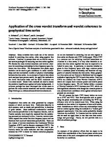
4.1. Adaptability of HPM-Based Wavelet Interpolation Operator. The first experiment image is a brain picture, which would be used to test the effectivness of the novel wavelet interpolation operator based on HPM. The result is shown in Figure 1. The image becomes more and more smooth with the image denoising processing, and the amount of the collocation points becomes less and less. Obviously, it is helpful to improve the efficiency of the algorithm. This shows that the operator constructed in this paper possesses the adaptability property. 4.2. Nonsensitivity to Time Step of the HPM-Based Wavelet Operator. The second image is solid circle with random noise. We try to illustrate the effectivness of the novel interpolation operator based on HPM comparing with the general operator. The results are shown in Figure 2. Using the novel HPM-based multilevel wavelet interpolation operator, the noise in images can be denoised rapidly. The denoising processing is slower with the original wavelet interpolation operator, and the image processing is less effective than that with the HPM-based multilevel wavelet interpolation operator on the same time step interval. One reason is because quasi-Shannon has no compact support property, and another is because the computational precision is so high that the noise is viewed as a part of the image. So, noises cannot be denoised rapidly. In addition, [32] has proved that HPM is not sensitive to the time step and is suitable for nonlinear equations.

Mathematical Problems in Engineering

(a0) Original image

7

(b0) Enhanced original image Original image

(a1) Original operator t = 0.00008, 𝜏 = 0.00002, k = 10

(b1) HPM-based operator t = 0.00008, 𝜏 = 0.00002, k = 10, r = 1

(a2) Original operator t = 0.0006, 𝜏 = 0.00002, k = 10, r = 1

(b2) HPM-based operator t = 0.0006, 𝜏 = 0.00002, k = 10, r = 1

(a3) Original operator t = 0.002, 𝜏 = 0.00002, k = 10

(b3) HPM-based operator t = 0.002, 𝜏 = 0.00002, k = 10, r = 1

(a4) Original operator t = 0.006, 𝜏 = 0.00002, k = 10

(b4) HPM-based operator t = 0.006, 𝜏 = 0.00002, k = 10, r = 1

Figure 2: Comparison about the denoising results between the general wavelet interpolation operator and the HPM-base multilevel wavelet interpolation operator.

8

Mathematical Problems in Engineering

(a1) t = 0.00005, 𝜏 = 0.00005

(b1) t = 0.00003, 𝜏 = 0.00003

(a2) t = 0.0001, 𝜏 = 0.00005

(b2) t = 0.00012, 𝜏 = 0.00003

(a3) t = 0.0002, 𝜏 = 0.00005

(b3) t = 0.00021, 𝜏 = 0.00003

(a) HPM-based wavelet interpolation operator

(b) Finite difference operator

Figure 3: The comparison about the smoothing result applying HAM.

4.3. Comparison between the Wavelet Interpolation Operator and the Finite Difference Operator. The third experiment image is a Metarhizium anisopliae picture, which would be used to test the effective of the novel wavelet interpolation operator based on HPM comparing with the finite difference operator. The result is shown in Figure 3. Although the time step of the difference method (𝜏 = 0.00003) is smaller than the wavelet method (𝜏 = 0.00005), the artifacts appeared in the denoising results with the difference method (Figures 3(b2) and 3(b3)), which is restricted by the wavelet interpolation method. It is well known that the basic function of the finite difference operator does not have the

property of smoothness, and so taking smaller time step is the only way to restrict the artifacts in processed images. The wavelet function possesses merits of smoothness and compact support, which are helpful to avoid the artifacts. It is obvious that this can be used to improve the efficiency of the algorithm.

5. Conclusions We have introduced HPM into the construction of the dynamic wavelet interpolation operator. The experiments illustrate it is a better idea to consider the wavelet transform

Mathematical Problems in Engineering as a nonlinear processing. HPM-based wavelet interpolation operator possesses the adaptability and nonsensitivity to the time step. In addition, comparing to the difference method which is widely used in solving P-M model in recent years, the wavelet numerical method can restrict the artifacts appearing in the processed images. Obviously, all of these can be used to improve the efficiency of the algorithm. As a preprocessing step, it makes the thinning and linking of the edges unnecessary, it preserves the edge junctions, and it does not require a complicated comparison of images at different scales since shape and position are preserved at every single scale. We believe that this will prove useful in many tasks of image processing.

Acknowledgments This work is supported by the National Key Technologies R & D Program of China under Grant no. 2012BAD35B02 and the National Natural Science Foundation of China under Grant no. 41171337.

References [1] P. Perona and J. Malik, “Scale-space and edge detection using anisotropic diffusion,” IEEE Transactions on Pattern Analysis and Machine Intelligence, vol. 12, no. 7, pp. 629–639, 1990. [2] Z. Guo, J. Sun, D. Zhang, and B. Wu, “Adaptive Perona-Malik model based on the variable exponent for image denoising,” IEEE Transactions on Image Processing, vol. 21, no. 3, pp. 958– 967, 2012. [3] X. Zhang and X. Feng, “Texture preserving Perona-Malik model,” in Proceedings of the 4th International Congress on Image and Signal Processing (CISP ’11), vol. 2, pp. 812–815, October 2011. [4] C. Lopez-Molina, B. de Baets, J. Cerron et al., “A generalization of the Perona-Malik anisotropic diffusion method using restricted dissimilarity functions,” International Journal of Computational Intelligence Systems, vol. 6, no. 1, pp. 14–28, 2013. [5] I. Daubechies and G. Teschke, “Variational image restoration by means of wavelets: simultaneous decomposition, deblurring, and denoising,” Applied and Computational Harmonic Analysis, vol. 19, no. 1, pp. 1–16, 2005. [6] I. Daubechies and G. Teschke, “Wavelet based image decomposition by variational functionals,” in Wavelet Applications in Industrial Processing, vol. 5266 of Proceedings of SPIE, pp. 94– 105, October 2003. [7] S. L. Mei, Q. S. Lu, S. W. Zhang, and L. Jin, “Adaptive interval wavelet precise integration method for partial differential equations,” Applied Mathematics and Mechanics, vol. 26, no. 3, pp. 333–340, 2005. [8] S.-L. Mei, Q.-S. Lu, and S.-W. Zhang, “Adaptive wavelet precise integration method for partial differential equations,” Chinese Journal of Computational Physics, vol. 21, no. 6, pp. 523–530, 2004. [9] S. Liao, Beyond Perturbation: Introduction to the Homotopy Analysis Method, CRC Press, 2004. [10] S. Liao, “Notes on the homotopy analysis method: some definitions and theorems,” Communications in Nonlinear Science and Numerical Simulation, vol. 14, no. 4, pp. 983–997, 2009.

9 [11] S.-J. Liao and K. F. Cheung, “Homotopy analysis of nonlinear progressive waves in deep water,” Journal of Engineering Mathematics, vol. 45, no. 2, pp. 105–116, 2003. [12] Y. Zhao, Z. Lin, Z. Liu, and S. Liao, “The improved homotopy analysis method for the Thomas-Fermi equation,” Applied Mathematics and Computation, vol. 218, no. 17, pp. 8363–8369, 2012. [13] O. Martin, “On the homotopy analysis method for solving a particle transport equation,” Applied Mathematical Modelling, vol. 37, no. 6, pp. 3959–3967, 2013. [14] G. Domairry, A. Mohsenzadeh, and M. Famouri, “The application of homotopy analysis method to solve nonlinear differential equation governing Jeffery-Hamel flow,” Communications in Nonlinear Science and Numerical Simulation, vol. 14, no. 1, pp. 85–95, 2009. [15] J.-H. He, “The homotopy perturbation method nonlinear oscillators with discontinuities,” Applied Mathematics and Computation, vol. 151, no. 1, pp. 287–292, 2004. [16] J.-H. He, “Homotopy perturbation method for bifurcation of nonlinear problems,” International Journal of Nonlinear Sciences and Numerical Simulation, vol. 6, no. 2, pp. 207–208, 2005. [17] J.-H. He, “Asymptotic methods for solitary solutions and compactons,” Abstract and Applied Analysis, vol. 2012, Article ID 916793, 130 pages, 2012. [18] J.-H. He, “Addendum: new interpretation of homotopy perturbation method,” International Journal of Modern Physics B, vol. 20, no. 18, pp. 2561–2568, 2006. [19] L. Cveticanin, “Homotopy-perturbation method for pure nonlinear differential equation,” Chaos, Solitons and Fractals, vol. 30, no. 5, pp. 1221–1230, 2006. [20] S. Abbasbandy, “Application of He’s homotopy perturbation method for Laplace transform,” Chaos, Solitons and Fractals, vol. 30, no. 5, pp. 1206–1212, 2006. [21] M. Rafei and D. D. Ganji, “Explicit solutions of Helmholtz equation and fifth-order KdV equation using homotopy perturbation method,” International Journal of Nonlinear Sciences and Numerical Simulation, vol. 7, no. 3, pp. 321–328, 2006. [22] A. M. Siddiqui, R. Mahmood, and Q. K. Ghori, “Thin film flow of a third grade fluid on a moving belt by he’s homotopy perturbation method,” International Journal of Nonlinear Sciences and Numerical Simulation, vol. 7, no. 1, pp. 7–14, 2006. [23] A. R. Ghotbi, H. Bararnia, G. Domairry, and A. Barari, “Investigation of a powerful analytical method into natural convection boundary layer flow,” Communications in Nonlinear Science and Numerical Simulation, vol. 14, no. 5, pp. 2222–2228, 2009. [24] S. H. Hosein Nia, A. N. Ranjbar, D. D. Ganji, H. Soltani, and J. Ghasemi, “Maintaining the stability of nonlinear differential equations by the enhancement of HPM,” Physics Letters A, vol. 372, no. 16, pp. 2855–2861, 2008. [25] M. Esmaeilpour and D. D. Ganji, “Application of He’s homotopy perturbation method to boundary layer flow and convection heat transfer over a flat plate,” Physics Letters A, vol. 372, no. 1, pp. 33–38, 2007. [26] H. Yan, “Adaptive wavelet precise integration method for nonlinear Black-Scholes model based on variational iteration method,” Abstract and Applied Analysis, vol. 2013, Article ID 735919, 6 pages, 2013. [27] R. Y. Xing, “Wavelet-based homotopy analysis method for nonlinear matrix system and its application in burgers equation,” Mathematical Problems in Engineering, vol. 2013, Article ID 982810, 7 pages, 2013.

10 [28] D. C. Wan and G. W. Wei, “The study of quasi wavelets based numerical method applied to Burgers’ equations,” Applied Mathematics and Mechanics, vol. 21, no. 10, pp. 991–1001, 2000. [29] G. W. Wei, “Quasi wavelets and quasi interpolating wavelets,” Chemical Physics Letters, vol. 296, no. 3-4, pp. 253–258, 1998. [30] S.-L. Mei, “Construction of target controllable image segmentation model based on homotopy perturbation technology,” Abstract and Applied Analysis, vol. 2013, Article ID 131207, 8 pages, 2013. [31] S.-L. Mei, C.-J. Du, and S.-W. Zhang, “Asymptotic numerical method for multi-degree-of-freedom nonlinear dynamic systems,” Chaos, Solitons and Fractals, vol. 35, no. 3, pp. 536–542, 2008. [32] S. Mei, S. Zhang, and Q. Lu, “Wavelet precise integration method for burgers equations based on homotopy technique,” Chinese Journal of Computational Physics, vol. 24, no. 1, pp. 54– 58, 2007.

Mathematical Problems in Engineering

Advances in

Operations Research Hindawi Publishing Corporation http://www.hindawi.com

Volume 2014

Advances in

Decision Sciences Hindawi Publishing Corporation http://www.hindawi.com

Volume 2014

Journal of

Applied Mathematics

Algebra

Hindawi Publishing Corporation http://www.hindawi.com

Hindawi Publishing Corporation http://www.hindawi.com

Volume 2014

Journal of

Probability and Statistics Volume 2014

The Scientific World Journal Hindawi Publishing Corporation http://www.hindawi.com

Hindawi Publishing Corporation http://www.hindawi.com

Volume 2014

International Journal of

Differential Equations Hindawi Publishing Corporation http://www.hindawi.com

Volume 2014

Volume 2014

Submit your manuscripts at http://www.hindawi.com International Journal of

Advances in

Combinatorics Hindawi Publishing Corporation http://www.hindawi.com

Mathematical Physics Hindawi Publishing Corporation http://www.hindawi.com

Volume 2014

Journal of

Complex Analysis Hindawi Publishing Corporation http://www.hindawi.com

Volume 2014

International Journal of Mathematics and Mathematical Sciences

Mathematical Problems in Engineering

Journal of

Mathematics Hindawi Publishing Corporation http://www.hindawi.com

Volume 2014

Hindawi Publishing Corporation http://www.hindawi.com

Volume 2014

Volume 2014

Hindawi Publishing Corporation http://www.hindawi.com

Volume 2014

Discrete Mathematics

Journal of

Volume 2014

Hindawi Publishing Corporation http://www.hindawi.com

Discrete Dynamics in Nature and Society

Journal of

Function Spaces Hindawi Publishing Corporation http://www.hindawi.com

Abstract and Applied Analysis

Volume 2014

Hindawi Publishing Corporation http://www.hindawi.com

Volume 2014

Hindawi Publishing Corporation http://www.hindawi.com

Volume 2014

International Journal of

Journal of

Stochastic Analysis

Optimization

Hindawi Publishing Corporation http://www.hindawi.com

Hindawi Publishing Corporation http://www.hindawi.com

Volume 2014

Volume 2014