We present a compact representation for human action recognition in videos using line and optical flow histograms. We introduce a new shape descriptor based ...
Human Action Recognition with Line and Flow Histograms Nazli Ikizler, R. Gokberk Cinbis and Pinar Duygulu Bilkent University, Dept of Computer Engineering, 06800, Ankara, Turkey {inazli,cinbis,duygulu}@bilkent.edu.tr Abstract We present a compact representation for human action recognition in videos using line and optical flow histograms. We introduce a new shape descriptor based on the distribution of lines which are fitted to boundaries of human figures. By using an entropy-based approach, we apply feature selection to densify our feature representation, thus, minimizing classification time without degrading accuracy. We also use a compact representation of optical flow for motion information. Using line and flow histograms together with global velocity information, we show that high-accuracy action recognition is possible, even in challenging recording conditions. 1
1. Introduction Human action recognition has gained a lot of interest during the past decade. From visual surveillance to humancomputer interaction systems, understanding what the people are doing is a necessary thread. However, making this thread fast and reliable still remains as an open research problem for the computer vision community. In order to achieve fast and reliable human action recognition, we should first search for the answer of the question “What is the best and minimal representation for actions?”. While there isn’t a current “best” solution to this problem, there are many efforts. Recent approaches extract “global” or “local” features, either on the spatial or on temporal domain, or both. Gavrila present an extensive survey over this subject in [6]. The approaches in genereal, tend to fall into three categories. First one includes explicit authoring of the temporal relations, whereas the second one uses explicit dynamical models. Such models can be constructed as hidden markov models ([3]), CRFs [17], or finite state models [7]. These models require a good deal of training data for reliable modeling. Ikizler and Forsyth [9] make use of motion capture data to overcome this data shortage. 1 This research is partially supported by TUBITAK Career grant 104E065 and grants 104E077 and 105E065.
Third approach is using the spatio-temporal templates, as Polana and Nelson [15] and Bobick and Davis [2]. Efros et al. [5] use a motion descriptor based on optical flow of a spatio-temporal volume. Blank et al. [1] define actions as space-time shapes. A recent approach based on a hierarchical use of spatio-temporal templates tries to model the ventral system of the brain to identify actions [10]. Recently, the ‘bag-of-words’ approaches, mostly based on forming codebooks of spatio-temporal features, are being adapted to action recognition. Laptev et al. first introduced the notion of ‘space-time interest points’ [12] and used SVMs to recognize actions [16]. Doll´ar et al. extracted cuboids via separable linear filters and formed histograms of these cuboids to perform action recognition [4]. Niebles et al. applied a pLSA approach over these patches [14]. Wong et al. proposed using pLSA with an implicit shape model to infer actions from spatio-temporal codebooks [18]. In this paper, we show how we can make use of a new shape descriptor together with a dense representation of optical flow and global temporal information for robust human action recognition. Our representation involves a very compact form, reducing the amount of classification time to a great extent. In this study, we use rbf kernel SVMs in the classification step, and present successful results over the state-of-art KTH dataset [16].
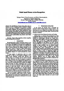
2. Our approach 2.1. Line-based shape features Shape is an important cue for recognizing the ongoing activity. In this study, we propose to use a compact shape representation based on lines. We extract this representation as follows: First, given a video sequence, we compute the probability of boundaries (Pb features [13]) based on Canny edges in each frame. We use these Pb features rather than simple edge detection, because Pb features delineate the boundaries of objects more strongly and eliminate the effect of noise caused by shorter edge segments in cluttered backgrounds to a certain degree. Example images and
their corresponding boundaries are shown in Fig 1(a) and Fig 1(b). After finding the boundaries, we localize the human figure by using the densest area of high response Pb features. We then fit straight lines to these boundaries using Hough transform. We do this in two-fold; first, we extract shorter lines (Fig 1(c)) to capture fine details of the human pose. Second, we extract relatively longer lines (Fig 1(d)) to capture the coarser shape information.
We calculate the entropy of the features as follows: Let fj (t) represent the feature vector of frame at time t in video j and let |Vj | denote the length of the video. The entropy H(fjn ) of each feature n over the temporal domain is H(fjn ) = −
|Vj | �
fˆjn (t)log(fˆjn (t))
where fˆ is the normalized feature over time such that fjn (t) fˆjn = �|V | j n t=1 fj (t)
(a)
(b)
(c)
(d)
Figure 1. Extraction of line-based features We then histogram the union of short and long line sets based on their orientations and spatial locations. The lines are histogrammed over 15◦ orientations, resulting in 12 circular bins. In order to incorporate spatial information of the human body, we evaluate these orientations within a N × N grid placed over the whole body. Our experiments show that N = 3 gives the best results (in accordance with [8]). This process is shown in Fig 2. Resulting shape feature vector is the concatenation of all bins, having a length |Q| = 108 where Q is the set of all features. 40 35 30 25 20 15 10 5 0
0
20
40
60
80
100
Figure 2. Forming line histograms
2.2. Feature Selection In our experiments, we observed that, even a feature size of |Q| = 108 is a sparse representation for shape. That is, based on the nature of the actions, some of the dimensions of this feature vector are hardly used. To have a more dense and compact representation and to reduce the processing time in classification step, we make use of an entropy-based feature selection approach. By selecting features with high entropy, we are able to detect regions of interest in which most of the change, i.e motion occurs.
(1)
t=1
(2)
This entropy H(fjn ) is a quantative measure of energy in a single feature dimension n. A low H(fjn ) means that the nth feature is stable during the action and higher H(fjn ) means the nth feature is changing rapidly in the presence of action. We expect that the high entropy features will be different for different action classes. Based on this observation, we compute the entropies of each feature in all training videos separately for each action. More formally, our reduced feature set Q� is � � Q� = f n |H(fjn ) > τ , ∀j ∈ {1, .., M }, n ∈ {1, .., |Q|} (3) where τ is the entropy threshold, M is the total number of videos in training set and Q is the original set of features. After this feature reduction step, our shape feature vector’s length reduces to ∼ 30. Note that for each action, we now have a separate set of features.
2.3. Motion features Using pure optical flow (OF) templates increase the size of the feature vector to a great extent. Instead, we present a compact OF representation for efficient action recognition. With this intention, we first extract dense block-based OF of each frame, by matching it to the previous frame. We then form orientation histograms of these OF values. This is similar to motion descriptors of Efros et al. [5], however we use spatial and directional binning. For each ith spatial bin where i ∈ {1, .., N × N } and direction θ ∈ {0, 90, 180, 270}, we define optical flow histogram hi (θ) such that � hi (θ) = ψ(˜ uθ · Fj ) (4) j∈Bi
where Fj represents the flow value in each pixel j, Bi is the set of pixels in the spatial bin i, u˜θ is the unit vector in θ direction and ψ function is defined as � � 0 if x ≤ 0 ψ(x) = (5) x if x > 0 This process is depicted in Fig 3.
SVMs for actions ak ∈ A� as our classification decision. The overall system is summarized in Fig. 4. 0.4 0.35 0.3
0.4
0.25
0.35
0.2
0.3
0.15
0.25
0.4 0.35 0.1
0.2
0.05
0.15
0.3 0.25 0
0
0.1 20
0.240
60
80
100
120
40
60
80
100
120
20
40
60
80
100
0.05 0.15
dx/dt
0
0
0.120 0.05 0
Figure 3. Forming OF histograms
0
120
velocity GMs
a1 a2
3. Recognizing Actions
an
LHist
3.1. SVM classification a1 a2
After the feature extraction step, we use them for the recognition of actions. We train separate shape and motion classifiers and combine the decisions of these by a majority voting scheme. For this purpose, we use SVM classifiers. We train separate one-vs-all SVM classifiers for each action. These SVM classifiers are formed using rbf kernels over snippets of frames using a windowing approach. In our windowing approach, the sequence is segmented into k-length chunks with some overlapping ratio o, then these chunks are classified individually (we achieved the best results with k = 7 , and o = 3). We combine the vote vectors from the shape cs and motion cm classifiers using a linear weighting scheme and obtain the final classification decision in cf , such that cf = α cs + (1 − α)cm
(6)
and we choose the action having the maximum vote in cf . We evaluate the effect of chosing α in the Section 4.
an
SVM models OFHist
Figure 4. Overall system architecture with addition of mean horizontal velocity.
4. Experimental Results Dataset: We tested our action recognition algorithm over the KTH dataset [16]. This is a challenging dataset, covering 25 subjects and 4 different recording conditions of the videos. There are 6 actions in this dataset: boxing, handclapping, handwaving, jogging, running and walking. We use the train and test sets provided in the original release of the dataset. Example frames from this dataset for each recording condition are shown in Fig. 5.
3.2. Including Global Temporal Information In addition to our local motion information (i.e. OF histograms), we also enchance the performance of our algorithm by using an additional global velocity information. Here, we propose to use a simple feature, which is the overall velocity of the subject in motion. Suppose we want to discriminate two actions: “handwaving” versus “running”. If the velocity of the person in motion is equal to zero, the probability that he is running is quite low. Based on this observation, we propose a two-level classification system. In the first level, we calculate mean velocities of the training sequences and fit a univariate Gaussian to each action in action set A = {a1 ..an } . Given a test instance, we compute the posterior probability of each action ai ∈ A over these Gaussians, and if the posterior probability of ai is greater than a threshold t (we use a loose bound t = 0.1), then we add ai to the probable set A� of actions for that sequence. After this preprocessing step, as the second level, we evaluate the sequences using our shape and motion descriptor. We take the maximum response of the
(a) s1: outdoor
(b) s2: different viewpoints
(c) s3: varying outfits/items
(d) s4: indoor
Figure 5. Different conditions of the KTH dataset [16].
Results: In Fig 6(a), we first show the effect of adding global velocity information. Here, LF corresponds to using line and flow histograms without the velocity information, and LFV is with global velocity. We observe that using global information gives a slight improvement on the overall accuracy. We also evaluate the effect of choosing α of Eq. 6. In this figure, α = 0 indicates that only motion features are used, whereas α = 1 corresponds to using only shape features. Our results show that α = 0.5 gives the best combination. The respective confusion matrix is shown in
Table 1. Comparison of our method to other methods on KTH dataset. Method Kim [11] Our method Jhuang [10] Wong [18] Niebles [14] Doll´ar [4] Schuldt [16]
Accuracy 95.33% 94.0% 91.7% 91.6% 81.5% 81.2% 71.7%
References
Table 2. Comparison by recording condition Condition s1 s2 s3 s4
Our Method 98.2% 90.7% 88.9% 98.2%
Jhuang [10] 96.0% 86.1% 89.8% 94.8%
Fig 6(b). Most of the confusion occurs between jog and run actions which are very similar in nature. 1 LFV LF
0.98 0.96
boxing
0.97
0.03
0.0
0.0
0.0
0.0
hclapping
0.06
0.89
0.06
0.0
0.0
0.0
hwaving
0.03
0.06
0.92
0.0
0.0
0.0
jogging
0.0
0.0
0.0
0.92
0.0
0.08
running
0.0
0.0
0.0
0.14
0.83
0.03
walking
0.03
0.0
0.0
0.03
0.0
0.94
accuracy
0.94 0.92 0.9 0.88
(a)
ng
g
w
al
ki
in nn ru
jo
gg
in
in
in
g
g
1
av
0.8
pp
0.6
la
α
hw
0.4
ng
0.2
xi
0
bo
0.8
hc
0.82
g
0.86 0.84
duce the classification time substantially. Within this framework, one can easily utilize more complicated classification schemes, which may further boost up the classifier performance. In addition, with achieving one of the best accuracies on the KTH dataset, we show that our novel shape and motion descriptor is quite successful in recognition of actions.
(b)
Figure 6. Choice of α and resulting confusion matrix for the KTH dataset. In Table 1, we compare our method’s performance to all major results on the KTH dataset reported so far (to the best of our knowledge). We achieve one of the highest accuracies (94%) on this state-of-art dataset, which shows that our approach successfully discriminates action instances. We also present accuracies for different recording conditions of the dataset in Table 2. Our approach outperforms the results of [10] (which reports performance for separate conditions) in three out of four of the conditions. Without feature selection, the total classification time (model construction and testing) of our approach is 26.47min. Using feature selection, this time drops to 15.96min. As expected, we gain considerable amount of time as we use a more compact feature representation.
5. Discussions and Conclusion In this paper, we present a compact representation for human action recognition using line and optical flow histograms. By using this compact representation, we re-
[1] M. Blank, L. Gorelick, E. Shechtman, M. Irani, and R. Basri. Actions as space-time shapes. In ICCV, pages 1395–1402, 2005. [2] A. Bobick and J. Davis. The recognition of human movement using temporal templates. PAMI, 23(3):257–267, 2001. [3] M. Brand, N. Oliver, and A. Pentland. Coupled hidden markov models for complex action recognition. In CVPR, pages 994–999, 1997. [4] P. Doll´ar, V. Rabaud, G. Cottrell, and S. Belongie. Behavior recognition via sparse spatio-temporal features. In VSPETS, October 2005. [5] A. A. Efros, A. C. Berg, G. Mori, and J. Malik. Recognizing action at a distance. In ICCV ’03, pages 726–733, 2003. [6] D. M. Gavrila. The visual analysis of human movement: A survey. CVIU, 73(1):82–98, 1999. [7] S. Hongeng, R. Nevatia, and F. Bremond. Video-based event recognition: activity representation and probabilistic recognition methods. CVIU, 96(2):129–162, November 2004. [8] N. Ikizler and P. Duygulu. Human action recognition using distribution of oriented rectangular patches. In Human Motion Workshop LNCS 4814, pages 271–284, 2007. [9] N. Ikizler and D. Forsyth. Searching video for complex activities with finite state models. CVPR, June 2007. [10] H. Jhuang, T. Serre, L. Wolf, and T. Poggio. A biologically inspired system for action recognition. In ICCV, 2007. [11] T. Kim, S. Wong, and R. Cipolla. Tensor canonical correlation analysis for action classification. In IEEE Conf. on Computer Vision and Pattern Recognition, pages 1–8, 2007. [12] I. Laptev and T. Lindeberg. Space-time interest points. In ICCV, page 432, 2003. [13] D. Martin, C. Fowlkes, and J. Malik. Learning to detect natural image boundaries using local brightness, color and texture cues. PAMI, 26, 2004. [14] J. C. Niebles, H. Wang, and L. Fei-Fei. Unsupervised learning of human action categories using spatial-temporal words. In BMVC, 2006. [15] R. Polana and R. Nelson. Detecting activities. In CVPR, pages 2–7, 1993. [16] C. Schuldt, I. Laptev, and B. Caputo. Recognizing human actions: A local svm approach. In ICPR, pages 32–36, Washington, DC, USA, 2004. IEEE Computer Society. [17] C. Sminchisescu, A. Kanaujia, Z. Li, and D. Metaxas. Conditional random fields for contextual human motion recognition. In ICCV, pages 1808–1815, 2005. [18] S.-F. Wong, T.-K. Kim, and R. Cipolla. Learning motion categories using both semantic and structural information. CVPR, June 2007.