Hybrid Geo-Spatial Query Processing on the Semantic Web - ORCA

Hybrid Geo-Spatial Query Processing on the Semantic Web

A thesis submitted in partial fulfilment of the requirement for the degree of Doctor of Philosophy

Eman M.G.Younis

2013

Cardiff University School of Computer Science & Informatics

iii

Declaration This work has not previously been accepted in substance for any degree and is not concurrently submitted in candidature for any degree. Signed . . . . . . . . . . . . . . . . . . . . . . . . . . . . . . . . . . . . . . . . . . . . . (candidate) Date

.................................

Statement 1 This thesis is being submitted in partial fulfillment of the requirements for the degree of PhD. Signed . . . . . . . . . . . . . . . . . . . . . . . . . . . . . . . . . . . . . . . . . . . . . (candidate) Date

.................................

Statement 2 This thesis is the result of my own independent work/investigation, except where otherwise stated. Other sources are acknowledged by explicit references. Signed . . . . . . . . . . . . . . . . . . . . . . . . . . . . . . . . . . . . . . . . . . . . . (candidate) Date

.................................

I hereby give consent for my thesis, if accepted, to be available for photocopying and for interlibrary loan, and for the title and summary to be made available to outside organisations. Signed . . . . . . . . . . . . . . . . . . . . . . . . . . . . . . . . . . . . . . . . . . . . . (candidate) Date

.................................

iv

v

Abstract Semantic Web data sources such as DBpedia are a rich resource of structured representations of knowledge about geographical features and provide potential data for computing the results of Question Answering System queries that require geo-spatial computations. Retrieval from these resources of all content that is relevant to a particular spatial query of, for example, containment, proximity or crossing is not always straightforward as the geometry is usually confined to point representations and there is considerable inconsistency in the way in which geographical features are referenced to locations. In DBpedia, some geographical feature instances have point coordinates, others have qualitative properties that provide explicit or implicit spatial relationships between named places, and some have neither of these. This thesis demonstrates that structured geo-spatial query, a form of question answering, on DBpedia can be performed with a hybrid query method that exploits quantitative and qualitative spatial properties in combination with a high quality reference geo-dataset that can help to support a full range of geo-spatial query operators such as proximity, containment and crossing as well as vague directional queries such as Find airports north of London?. A quantitative model based on the spatial directional relations in DBpedia has been used to assist in query processing. Evaluation experiments confirm the benefits of combining qualitative and quantitative methods for containment queries and of employing high-quality spatial data, as opposed to DBpedia points, as reference objects for proximity queries, particularly for linear features. The high quality geo-data also enabled answering questions impossible to answer with Semantic Web resources alone, such as finding geographic features within some distance from a region boundary. The contributions were validated by a prototype geo-spatial query system that combined qualitative and quantitative processing and included ranking answers for directional queries based on models derived from DBpedia contributed data.

vi

Abstract

vii

Acknowledgements I would like to express my gratitude and deepest thanks to Allah (GOD) for giving me the ability to complete this work. I would like also to thank all the people who helped and supported me and stood by me throughout my PhD study, but I wish to particularly acknowledge a number of people who had a great impact on my thesis. First of all, I am really thankful to my great supervisors, professor Chris Jones and Dr. Alia Abdelmoty, whose encouragement, guidance and support helped me to acquire new research skills and a deeper understanding of the field. Their experience and knowledge, endless help and advice to me made my research exciting and interesting. This is also an opportunity for me to extend my thanks to my employer Minia University, and the cultural office in London for awarding me the scholarship, and providing all the required financial support to complete my degree. I cannot ignore the technical and scientific support of the School of Computer Science & Informatics at Cardiff University, UK and all its staff members and all my colleagues in the school. Last but not least, I owe my deepest gratitude and thanks to my lovely, kind mother, my kind, patient husband, my lovely twins (Mariem and Malak)and my little one Emy, for their continuous and endless help, encouragement and support during the stressful times of my study. Finally, I would like to thank anyone who provided any help or support for me during my time of study at Cardiff University.

viii

Acknowledgements

ix

Contents

Abstract

v

Acknowledgements

vii

Contents

ix

List of Figures

xv

List of Tables

xxi

List of abbreviations

xxv

1

Introduction

1

1.1

Overview and Research Context . . . . . . . . . . . . . . . . . . . . . . . . .

1

1.2

Motivation . . . . . . . . . . . . . . . . . . . . . . . . . . . . . . . . . . . . .

4

1.3

Scope . . . . . . . . . . . . . . . . . . . . . . . . . . . . . . . . . . . . . . .

6

1.4

Research Hypothesis . . . . . . . . . . . . . . . . . . . . . . . . . . . . . . .

7

1.5

Research Questions . . . . . . . . . . . . . . . . . . . . . . . . . . . . . . . .

7

1.6

Thesis Contributions . . . . . . . . . . . . . . . . . . . . . . . . . . . . . . .

8

1.7

Thesis Organisation . . . . . . . . . . . . . . . . . . . . . . . . . . . . . . . .

9

1.8

Summary . . . . . . . . . . . . . . . . . . . . . . . . . . . . . . . . . . . . .

10

x 2

3

Contents Background

11

2.1

Introduction . . . . . . . . . . . . . . . . . . . . . . . . . . . . . . . . . . . .

11

2.2

Semantic Web Overview . . . . . . . . . . . . . . . . . . . . . . . . . . . . .

11

2.3

The Semantic Web Technologies . . . . . . . . . . . . . . . . . . . . . . . . .

12

2.3.1

Resource Description Framework (RDF) . . . . . . . . . . . . . . . .

13

2.3.2

RDF serialisation formats . . . . . . . . . . . . . . . . . . . . . . . .

14

2.3.3

Ontologies . . . . . . . . . . . . . . . . . . . . . . . . . . . . . . . .

15

2.3.4

SPARQL . . . . . . . . . . . . . . . . . . . . . . . . . . . . . . . . .

16

2.4

Linked Data . . . . . . . . . . . . . . . . . . . . . . . . . . . . . . . . . . . .

17

2.5

Geo-spatial linked datasets . . . . . . . . . . . . . . . . . . . . . . . . . . . .

20

2.6

DBpedia . . . . . . . . . . . . . . . . . . . . . . . . . . . . . . . . . . . . . .

23

2.6.1

DBpedia extraction framework from Wikipedia . . . . . . . . . . . . .

23

2.6.2

DBpedia Extraction Modes . . . . . . . . . . . . . . . . . . . . . . . .

25

2.6.3

DBpedia Extraction Methods . . . . . . . . . . . . . . . . . . . . . . .

26

2.6.4

DBpedia Knowledge Base Specifications . . . . . . . . . . . . . . . .

27

2.7

DBpedia Applications . . . . . . . . . . . . . . . . . . . . . . . . . . . . . . .

29

2.8

Volunteered Geographical Information (VGI) . . . . . . . . . . . . . . . . . .

32

2.9

Spatial DBMS . . . . . . . . . . . . . . . . . . . . . . . . . . . . . . . . . . .

33

2.9.1

Geo-spatial data formats and geometry representation . . . . . . . . . .

34

2.9.2

Referencing systems . . . . . . . . . . . . . . . . . . . . . . . . . . .

34

2.10 Summary . . . . . . . . . . . . . . . . . . . . . . . . . . . . . . . . . . . . .

35

Related Research

37

3.1

Introduction . . . . . . . . . . . . . . . . . . . . . . . . . . . . . . . . . . . .

37

3.2

Geographic Information Retrieval(GIR) . . . . . . . . . . . . . . . . . . . . .

38

3.3

Question Answering Systems . . . . . . . . . . . . . . . . . . . . . . . . . . .

39

3.3.1

39

History of Question Answering Systems . . . . . . . . . . . . . . . . .

Contents 3.3.2

Question Answering Systems classifications . . . . . . . . . . . . . . .

40

3.3.3

General QAS Architecture . . . . . . . . . . . . . . . . . . . . . . . .

41

3.4

Question Answering Sites . . . . . . . . . . . . . . . . . . . . . . . . . . . . .

42

3.5

Geographic Question Answering Systems . . . . . . . . . . . . . . . . . . . .

43

3.6

Question Answering Systems on the Semantic Web . . . . . . . . . . . . . . .

45

3.7

Integrating Semantic Web data with geo-spatial data . . . . . . . . . . . . . . .

45

3.8

Geo-Spatial Extensions of SPARQL and RDF . . . . . . . . . . . . . . . . . .

46

3.8.1

GeoSPARQL and st-SPARQL . . . . . . . . . . . . . . . . . . . . . .

47

3.8.2

RDF triple Stores . . . . . . . . . . . . . . . . . . . . . . . . . . . . .

48

3.8.3

RDF Stores supporting geo-spatial extensions . . . . . . . . . . . . . .

49

Limitations of existing GQAS . . . . . . . . . . . . . . . . . . . . . . . . . .

50

3.10 Summary . . . . . . . . . . . . . . . . . . . . . . . . . . . . . . . . . . . . .

51

Geo-spatial Contents of DBpedia

53

4.1

Introduction . . . . . . . . . . . . . . . . . . . . . . . . . . . . . . . . . . . .

53

4.2

DBpedia Access Methods . . . . . . . . . . . . . . . . . . . . . . . . . . . . .

54

4.3

Geo-spatial Content of DBpedia . . . . . . . . . . . . . . . . . . . . . . . . .

55

4.3.1

Non-spatial properties in DBpedia . . . . . . . . . . . . . . . . . . . .

56

4.3.2

Spatial Properties in DBpedia . . . . . . . . . . . . . . . . . . . . . .

56

4.3.3

Spatial Relation Attributes . . . . . . . . . . . . . . . . . . . . . . . .

56

4.4

Evaluating the positional accuracy of DBpedia data points versus OS . . . . . .

62

4.5

Quantitative Analysis of DBpedia Directional Relations . . . . . . . . . . . . .

63

4.5.1

Overview . . . . . . . . . . . . . . . . . . . . . . . . . . . . . . . . .

63

4.5.2

Purpose . . . . . . . . . . . . . . . . . . . . . . . . . . . . . . . . . .

63

4.5.3

Data Collection . . . . . . . . . . . . . . . . . . . . . . . . . . . . . .

64

4.5.4

Data Cleaning and Calculations . . . . . . . . . . . . . . . . . . . . .

65

4.5.5

Data Analysis . . . . . . . . . . . . . . . . . . . . . . . . . . . . . . .

65

3.9

4

xi

xii

Contents

4.6 5

Results . . . . . . . . . . . . . . . . . . . . . . . . . . . . . . . . . .

66

4.5.7

Relationship between Distance and Angle . . . . . . . . . . . . . . . .

77

Summary . . . . . . . . . . . . . . . . . . . . . . . . . . . . . . . . . . . . .

83

System Analysis and Design

85

5.1

Introduction . . . . . . . . . . . . . . . . . . . . . . . . . . . . . . . . . . . .

85

5.2

System Analysis . . . . . . . . . . . . . . . . . . . . . . . . . . . . . . . . . .

85

5.2.1

Requirements Analysis - Problem Statement . . . . . . . . . . . . . .

85

System Design . . . . . . . . . . . . . . . . . . . . . . . . . . . . . . . . . .

86

5.3.1

System Architecture . . . . . . . . . . . . . . . . . . . . . . . . . . .

87

5.3.2

Database Design . . . . . . . . . . . . . . . . . . . . . . . . . . . . .

88

5.3.3

Query planner design . . . . . . . . . . . . . . . . . . . . . . . . . . .

89

5.3.4

Non-spatial questions query plan . . . . . . . . . . . . . . . . . . . . .

89

5.3.5

Spatial questions query plan . . . . . . . . . . . . . . . . . . . . . . .

90

5.3.6

Containment questions query plan . . . . . . . . . . . . . . . . . . . .

90

5.3.7

Directional questions query plan . . . . . . . . . . . . . . . . . . . . .

91

5.3.8

Crossing questions query plan . . . . . . . . . . . . . . . . . . . . . .

95

5.3.9

Proximity questions query plan . . . . . . . . . . . . . . . . . . . . .

96

5.3.10 User Interface Design . . . . . . . . . . . . . . . . . . . . . . . . . .

97

Summary . . . . . . . . . . . . . . . . . . . . . . . . . . . . . . . . . . . . .

97

5.3

5.4 6

4.5.6

Implementation

99

6.1

Introduction . . . . . . . . . . . . . . . . . . . . . . . . . . . . . . . . . . . .

99

6.2

Implementation Methodology . . . . . . . . . . . . . . . . . . . . . . . . . .

99

6.3

Implementation Overview . . . . . . . . . . . . . . . . . . . . . . . . . . . . 100

6.4

Spatially indexing DBpedia

6.5

Storing OS high quality mapping geo-data . . . . . . . . . . . . . . . . . . . . 105

6.6

Linking DBpedia spatially-indexed data with OS geo-data . . . . . . . . . . . 105

. . . . . . . . . . . . . . . . . . . . . . . . . . . 101

Contents

7

6.7

Implementing the user interface and query plans . . . . . . . . . . . . . . . . . 105

6.8

The prototype system in action . . . . . . . . . . . . . . . . . . . . . . . . . . 111

6.9

Summary . . . . . . . . . . . . . . . . . . . . . . . . . . . . . . . . . . . . . 117

Results and Evaluation

119

7.1

Introduction . . . . . . . . . . . . . . . . . . . . . . . . . . . . . . . . . . . . 119

7.2

Scenario 1: using DBpedia in answering geo-spatial questions . . . . . . . . . 120

7.3

Scenario 2: using a spatially-indexed version of DBpedia . . . . . . . . . . . . 121

7.4

Scenario 3: combining indexed-DBpedia with high-quality detailed geo-data . . 122

7.5

Scenario 4: integrating quantitative with qualitative spatial relations for answering containment questions . . . . . . . . . . . . . . . . . . . . . . . . . . . . 125

7.6

Evaluation of the effect of combining geo-data with DBpedia data for Proximity questions . . . . . . . . . . . . . . . . . . . . . . . . . . . . . . . . . . . . . 127

7.7

8

xiii

7.6.1

Evaluation experiment . . . . . . . . . . . . . . . . . . . . . . . . . . 127

7.6.2

Discussion . . . . . . . . . . . . . . . . . . . . . . . . . . . . . . . . 127

Evaluating the integration of quantitative and qualitative attributes in answering Containment questions . . . . . . . . . . . . . . . . . . . . . . . . . . . . . . 136 7.7.1

Evaluation Experiment . . . . . . . . . . . . . . . . . . . . . . . . . . 136

7.7.2

Discussion . . . . . . . . . . . . . . . . . . . . . . . . . . . . . . . . 136

7.8

Evaluating the Directional Relation Questions . . . . . . . . . . . . . . . . . . 145

7.9

Summary . . . . . . . . . . . . . . . . . . . . . . . . . . . . . . . . . . . . . 146

Conclusions and Future Work

149

8.1

Introduction . . . . . . . . . . . . . . . . . . . . . . . . . . . . . . . . . . . . 149

8.2

Answers to Research Questions . . . . . . . . . . . . . . . . . . . . . . . . . . 149

8.3

Conclusions . . . . . . . . . . . . . . . . . . . . . . . . . . . . . . . . . . . . 152 8.3.1

8.4

Summary of Contributions . . . . . . . . . . . . . . . . . . . . . . . . 153

Achievements . . . . . . . . . . . . . . . . . . . . . . . . . . . . . . . . . . . 153

xiv

Contents 8.5

Practical Implications and Future Work . . . . . . . . . . . . . . . . . . . . . 154

8.6

Summary . . . . . . . . . . . . . . . . . . . . . . . . . . . . . . . . . . . . . 156

Bibliography

157

Appendix A: Qualitative Spatial Attributes

175

Appendix B: Directional relations Online Survey

193

Appendix C: SQL and SPARQL Query examples

213

xv

List of Figures

1.1

Example of a proximity question asked to Google Maps, June 2013 . . . . . .

2

1.2

Examples of geo-spatial relationship questions that START QAS fails to answer, June 2013 . . . . . . . . . . . . . . . . . . . . . . . . . . . . . . . . . . . . .

5

An example of geo-spatial relationship questions that WalframeAlpa QAS fails to answer, June 2013 . . . . . . . . . . . . . . . . . . . . . . . . . . . . . . .

6

Relation between The Semantic Web - web of data - and the conventional web - web of documents from [74] . . . . . . . . . . . . . . . . . . . . . . . . . .

12

2.2

RDF graph representing facts from DBpedia about Wales . . . . . . . . . . . .

13

2.3

Example of RDF/XML representation format . . . . . . . . . . . . . . . . . .

14

2.4

A snapshot of DBpedia ontology Place Class . . . . . . . . . . . . . . . . . .

16

2.5

Linked data cloud data sets graph as in Sept 2011 [4] . . . . . . . . . . . . . .

19

2.6

Distribution of triples on Linked data by domain [1] . . . . . . . . . . . . . . .

21

2.7

DBpedia Extraction Framework from Wikipedia [25] . . . . . . . . . . . . . .

24

2.8

Infobox showing entities that have directional relations with Cardiff in Wikipedia 26

2.9

Screen shot for using RelFinder to find RDF relationships between Cardiff and the United Kingdom . . . . . . . . . . . . . . . . . . . . . . . . . . . . . . .

30

2.10 Spatial data representation from OGC simple feature specification [7] . . . . .

34

3.1

Areas related to the work of the thesis . . . . . . . . . . . . . . . . . . . . . .

37

4.1

Screen shot of DBpedia page describing a River, showing the quantitative and qualitative spatial attributes . . . . . . . . . . . . . . . . . . . . . . . . . . . .

55

1.3

2.1

xvi

List of Figures 4.2

Distance histograms for distances between LOs and ROs for predicates implying proximity nearN, nearS, nearE and nearW . . . . . . . . . . . . . . . . . .

58

4.3

Histogram for the distance in KM for North relation . . . . . . . . . . . . . . .

67

4.4

Histogram for the distance in KM for East relation . . . . . . . . . . . . . . .

67

4.5

Histogram for the distance in KM for West relation . . . . . . . . . . . . . . .

68

4.6

Histogram for the distance in KM for Northeast relation . . . . . . . . . . . . .

68

4.7

Histogram for the distance in KM for Southeast relation . . . . . . . . . . . . .

69

4.8

Histogram for the distance in KM for Southwest relation . . . . . . . . . . . .

69

4.9

Histogram for the accumulated distance in KM over all spatial directional relations 70

4.10 Box plot for the distance in KM for all spatial directional relations . . . . . . .

70

4.11 Box plot for the distance in KM for for small, medium and bigger places . . . .

71

4.12 Scatter plot for the relation between population and distances in KM between RO(s) and LO(s) for small places . . . . . . . . . . . . . . . . . . . . . . . . .

72

4.13 Scatter plot for the relation between population and distances in KM between RO(s) and LO(s) for medium size places . . . . . . . . . . . . . . . . . . . . .

72

4.14 Scatter plot for the relation between population and distances in KM between RO(s) and LO(s) for bigger places . . . . . . . . . . . . . . . . . . . . . . . .

73

4.15 Circular raw data Plot of the actual angle data for the four basic spatial directional relations (North, South, East and West) in DBpedia . . . . . . . . . . . .

74

4.16 Circular raw data plots for the actual angle data histograms for the four intermediate spatial directional relations (Northeast, Northwest, Southeast and Southwest) 75 4.17 Rose Diagram for the angles between the subject(s) and object(s) for the basic spatial directional relations (North, South, East and West) . . . . . . . . . . . .

76

4.18 Rose Diagram for the angles between the subject(s) and object(s) for the intermediate spatial directional relations (Northeast, Northwest, Southeast, and Southwest) . . . . . . . . . . . . . . . . . . . . . . . . . . . . . . . . . . . .

77

4.19 Scatter plot for the distance and angle between object and subject(s) for North relationship . . . . . . . . . . . . . . . . . . . . . . . . . . . . . . . . . . . .

79

4.20 Scatter density plot for the distance and angle between object and subject(s) for North relationship . . . . . . . . . . . . . . . . . . . . . . . . . . . . . . . . .

79

List of Figures

xvii

4.21 Scatter plot for the distance and angle between object and subject(s) for South relationship . . . . . . . . . . . . . . . . . . . . . . . . . . . . . . . . . . . .

80

4.22 Scatter density plot for the distance and angle between object and subject(s) for South relationship . . . . . . . . . . . . . . . . . . . . . . . . . . . . . . . . .

80

4.23 Scatter plot for the distance and angle between object and subject(s) for East relationship . . . . . . . . . . . . . . . . . . . . . . . . . . . . . . . . . . . .

81

4.24 Scatter density plot for the distance and angle between object and subject(s) for East relationship . . . . . . . . . . . . . . . . . . . . . . . . . . . . . . . . . .

81

4.25 Scatter plot for the distance and angle between object and subject(s) for West relationship . . . . . . . . . . . . . . . . . . . . . . . . . . . . . . . . . . . .

82

4.26 Scatter density plot for the distance and angle between object and subject(s) for West relationship . . . . . . . . . . . . . . . . . . . . . . . . . . . . . . . . .

82

5.1

Query Answering System Sequence Diagram . . . . . . . . . . . . . . . . . .

86

5.2

System Architecture . . . . . . . . . . . . . . . . . . . . . . . . . . . . . . . .

87

5.3

Database table design for the DBpedia data . . . . . . . . . . . . . . . . . . .

88

5.4

Database table design for the Ordnance Survey data . . . . . . . . . . . . . . .

88

5.5

Database table design for links between the DBpedia data and the OS geo-data

88

5.6

Activity diagram for non-spatial questions query plan . . . . . . . . . . . . . .

89

5.7

Activity diagram for spatial questions query plan . . . . . . . . . . . . . . . .

90

5.8

Activity diagram for containment questions query plan . . . . . . . . . . . . .

91

5.9

Activity diagram for the directional questions query plan . . . . . . . . . . . .

92

5.10 Acceptance and rejection regions for north relation . . . . . . . . . . . . . . .

93

5.11 Acceptance and rejection regions for south relation . . . . . . . . . . . . . . .

93

5.12 Acceptance and rejection regions for east relation . . . . . . . . . . . . . . . .

94

5.13 Acceptance and rejection regions for west relation . . . . . . . . . . . . . . . .

94

5.14 Activity diagram for query plan for crossing queries . . . . . . . . . . . . . . .

95

5.15 Activity diagram for query plan for proximity queries . . . . . . . . . . . . . .

96

5.16 User interface design . . . . . . . . . . . . . . . . . . . . . . . . . . . . . . .

97

xviii

List of Figures

6.1

Implementation Overview . . . . . . . . . . . . . . . . . . . . . . . . . . . . 100

6.2

Snapshot of Virtuoso DBpedia SPARQL Endpoint . . . . . . . . . . . . . . . . 104

6.3

Implementing the user interface . . . . . . . . . . . . . . . . . . . . . . . . . 106

6.4

Example of non-spatial questions . . . . . . . . . . . . . . . . . . . . . . . . . 112

6.5

Example of spatial questions . . . . . . . . . . . . . . . . . . . . . . . . . . . 112

6.6

Example of spatial questions . . . . . . . . . . . . . . . . . . . . . . . . . . . 113

6.7

Example of containment questions . . . . . . . . . . . . . . . . . . . . . . . . 113

6.8

Example of containment questions . . . . . . . . . . . . . . . . . . . . . . . . 114

6.9

Specifying distance in proximity question . . . . . . . . . . . . . . . . . . . . 114

6.10 Proximity question calculated from boundary . . . . . . . . . . . . . . . . . . 115 6.11 Proximity question calculated from centre . . . . . . . . . . . . . . . . . . . . 115 6.12 Example of crossing questions . . . . . . . . . . . . . . . . . . . . . . . . . . 116 6.13 Example of directional questions . . . . . . . . . . . . . . . . . . . . . . . . . 116 7.1

Results for the question Find hospitals within 10 KM of Cardiff? using DBpedia point for Cardiff . . . . . . . . . . . . . . . . . . . . . . . . . . . . . . . . . . 121

7.2

Results for the question Find hospitals within 10 KM of river Taff? using DBpedia point for river Taff . . . . . . . . . . . . . . . . . . . . . . . . . . . . . 122

7.3

Results for the question Find hospitals within 10 KM of Cardiff? using OS polygon representation for Cardiff . . . . . . . . . . . . . . . . . . . . . . . . 123

7.4

Results for the question Find hospitals within 10 KM of river Taff? using OS linear representation for river Taff . . . . . . . . . . . . . . . . . . . . . . . . 123

7.5

The total number of answers using OS detailed linear representation and DBpedia point representation as RO for rivers . . . . . . . . . . . . . . . . . . . . . 128

7.6

The total number of instances having spatial relation of containment (S), spatial containment relation and inside the boundary of the RO (SGi), those outside the boundary of the RO (SGn), with geographical coordinates (G), combined number of instances having either spatial containment relationships or geographic coordinates after removing duplicates (S∪G) . . . . . . . . . . . . . . . . . . . 137

List of Figures

xix

8.1

Survey page 1 . . . . . . . . . . . . . . . . . . . . . . . . . . . . . . . . . . . 194

8.2

Survey page 2-1

. . . . . . . . . . . . . . . . . . . . . . . . . . . . . . . . . 195

8.3

Survey page 2-2

. . . . . . . . . . . . . . . . . . . . . . . . . . . . . . . . . 196

8.4

Survey page 3-1

. . . . . . . . . . . . . . . . . . . . . . . . . . . . . . . . . 197

8.5

Survey page 3-2

. . . . . . . . . . . . . . . . . . . . . . . . . . . . . . . . . 198

8.6

Survey page 4-1

. . . . . . . . . . . . . . . . . . . . . . . . . . . . . . . . . 199

8.7

Survey page 4-2

. . . . . . . . . . . . . . . . . . . . . . . . . . . . . . . . . 200

8.8

Survey page 5-1

. . . . . . . . . . . . . . . . . . . . . . . . . . . . . . . . . 201

8.9

Survey page 5-2

. . . . . . . . . . . . . . . . . . . . . . . . . . . . . . . . . 202

8.10 Survey page 6 . . . . . . . . . . . . . . . . . . . . . . . . . . . . . . . . . . . 203 8.11 Rankings from the system for north . . . . . . . . . . . . . . . . . . . . . . . 204 8.12 Rankings from the system for south . . . . . . . . . . . . . . . . . . . . . . . 204 8.13 Rankings from the system for east . . . . . . . . . . . . . . . . . . . . . . . . 205 8.14 Rankings from the system for west

. . . . . . . . . . . . . . . . . . . . . . . 205

8.15 Survey Results 1 . . . . . . . . . . . . . . . . . . . . . . . . . . . . . . . . . 206 8.16 Survey Results 2 . . . . . . . . . . . . . . . . . . . . . . . . . . . . . . . . . 207 8.17 Survey Results 3 . . . . . . . . . . . . . . . . . . . . . . . . . . . . . . . . . 208 8.18 Survey Results 4 . . . . . . . . . . . . . . . . . . . . . . . . . . . . . . . . . 209 8.19 Survey Results 5 . . . . . . . . . . . . . . . . . . . . . . . . . . . . . . . . . 210 8.20 Survey Results 6 . . . . . . . . . . . . . . . . . . . . . . . . . . . . . . . . . 211

xx

List of Figures

xxi

List of Tables

4.1

Per class Properties that imply containment in DBpedia . . . . . . . . . . . . .

59

4.2

Per class Properties that imply containment in DBpedia. Cont . . . . . . . . . .

60

4.3

Spatial Directional relations in DBpedia for Cardiff . . . . . . . . . . . . . . .

61

4.4

Descriptive statistics showing the distance in kilometres between DBpedia points and OS points . . . . . . . . . . . . . . . . . . . . . . . . . . . . . . . . . . .

62

Summary statistics for distances in KM between subject(s) and object(s) for different spatial directional relations . . . . . . . . . . . . . . . . . . . . . . .

66

4.5

6.1

Per class number of instances in the DBpedia index . . . . . . . . . . . . . . . 104

7.1

Example of proximity questions using DBpedia point representation for the RO "Cardiff - River Taff" . . . . . . . . . . . . . . . . . . . . . . . . . . . . . . . 121

7.2

Example of proximity questions using OS polygonal representation for the RO "Cardiff - River Taff" . . . . . . . . . . . . . . . . . . . . . . . . . . . . . . . 124

7.3

Answers from quantitative and qualitative properties for a containment question 125

7.4

Examples of place URI in DBpedia, having coordinates without spatial containment relation predicates and vice versa . . . . . . . . . . . . . . . . . . . . . . 126

7.5

For each class, no of instances retrieved from DBpedia index, within distance(10 KM, 50 KM, 100 KM) from the RO (linear) features such as rivers using OS linear representation (OS) and DBpedia point representation (DB)of RO . . . . 129

7.6

For each class, no of instances retrieved from DBpedia index, within distance(10 KM, 50 KM, 100 KM) from the RO (Linear) features such as rivers using OS linear representation (OS) and DBpedia point representation (DB)of RO . . . . 130

xxii

List of Tables

7.7

For each class, no of instances retrieved from DBpedia index, within distance(10 KM, 50 KM, 100 KM) from the RO (Linear) features such as rivers using OS linear representation (OS) and DBpedia point representation (DB)of RO . . . . 131

7.8

For each class, no of instances retrieved from DBpedia index, within distance(10 KM, 50 KM, 100 KM) from the RO (Linear) features such as rivers using OS linear representation (OS) and DBpedia point representation (DB)of RO . . . . 132

7.9

For each class, no of instances retrieved from DBpedia index, within distance(10 KM, 50 KM, 100 KM) from the RO (Linear) features such as rivers using OS linear representation (OS) and DBpedia point representation (DB)of RO . . . . 133

7.10 For each class, no of instances retrieved from DBpedia index, within distance(10 KM, 50 KM, 100 KM) from the RO (Linear) features such as rivers using OS linear representation (OS) and DBpedia point representation (DB)of RO . . . . 134 7.11 For each class, no of instances retrieved from DBpedia index, within distance(10 KM, 50 KM, 100 KM) from the RO (Linear) features such as rivers using OS linear representation (OS) and DBpedia point representation (DB)of RO and Totals . . . . . . . . . . . . . . . . . . . . . . . . . . . . . . . . . . . . . . . 135 7.12 Per feature and per region, number of features related to it with spatial containment relations (S), those of S that fall within the boundaries of the RO (SGi), those do not (SGn). G represents all features with geographic coordinates which fall within the boundary. (S∪G), combined results from S and G, removing duplicates . . . . . . . . . . . . . . . . . . . . . . . . . . . . . . . . . . . . . . 138 7.13 Per feature and per region, number of features related to it with spatial containment relations (S), those of S that fall within the boundaries of the RO (SGi), those do not (SGn). G represents all features with geographic coordinates which fall within the boundary. (S∪G), combined results from S and G, removing duplicates. Cont . . . . . . . . . . . . . . . . . . . . . . . . . . . . . . . . . . . 139 7.14 Per feature and per region, number of features related to it with spatial containment relations (S), those of S that fall within the boundaries of the RO (SGi), those do not (SGn). G represents all features with geographic coordinates which fall within the boundary. (S∪G), combined results from S and G, removing duplicates. Cont . . . . . . . . . . . . . . . . . . . . . . . . . . . . . . . . . . . 140

List of Tables

xxiii

7.15 Per feature and per region, number of features related to it with spatial containment relations (S), those of S that fall within the boundaries of the RO (SGi), those do not (SGn). G represents all features with geographic coordinates which fall within the boundary. (S∪G), combined results from S and G, removing duplicates. Cont . . . . . . . . . . . . . . . . . . . . . . . . . . . . . . . . . . . 141 7.16 Per feature and per region, number of features related to it with spatial containment relations (S), those of S that fall within the boundaries of the RO (SGi), those do not (SGn). G represents all features with geographic coordinates which fall within the boundary. (S∪G), combined results from S and G, removing duplicates. Cont . . . . . . . . . . . . . . . . . . . . . . . . . . . . . . . . . . . 142 7.17 Per feature and per region, number of features related to it with spatial containment relations (S), those of S that fall within the boundaries of the RO (SGi), those do not (SGn). G represents all features with geographic coordinates which fall within the boundary. (S∪G), combined results from S and G, removing duplicates. Cont . . . . . . . . . . . . . . . . . . . . . . . . . . . . . . . . . . . 143 7.18 Per feature and per region, number of features related to it with spatial containment relations (S), those of S that fall within the boundaries of the RO (SGi), those do not (SGn). G represents all features with geographic coordinates which fall within the boundary. (S∪G), combined results from S and G, removing duplicates and Totals . . . . . . . . . . . . . . . . . . . . . . . . . . . . . . . . . 144

xxiv

List of Tables

xxv

List of abbreviations API Application Programming Interface csv comma separated values DBMS Data Base Management System E east GIR Geographic Information Retrieval GIS Geographic Information System GML Geography Mark up Language GPS Global Positioning System GQAS Geographic Question Answering Systems HTTP HyperText Transfer Protocol IR Information Retrieval KM Kilo meters lat latitude LD Linked Data LO Located object long longitude N north NE northeast NLP Natural Language Processing

xxvi NW northwest OGC The Open Geospatial Consortium OS Ordnance Survey,a digital mapping agency for the UK OSM OpenStreetMap QA Question Answering QAS Question Answering Systems RDF Resource Description Framework RO Reference Object S south SE southeast SQL Structured Query Language SW southwest UGC User Generated Content URI Universal Resource Identifier URL Uniform Resource Locators VGI Volunteered Geographical Information W west WKT Well Known Text WWW World Wide Web

List of abbreviations

1

Chapter 1

Introduction

1.1

Overview and Research Context

Spatially referenced information or geo-spatial information can be regarded as information which is associated with geometric coordinates in a specific reference system or with some other attribute that associates a geographic object with its location. Geo-spatial information is defined in [110] as spatial information, which is geo-referenced. Queries on geo-spatial information may be classified into spatial queries and non-spatial or thematic queries. Non-spatial queries are not related to the location of the object, whereas spatial queries can be either related to a spatial attribute such as the geometry of the object or to a spatial relation. Spatial relations can be categorised into topological, proximity and directional. Geo-spatial knowledge is a crucial component on the web and particularly on the Semantic Web as it is involved in all aspects of human-related activities[150]. Moreover, the availability of huge amounts of geo-spatial knowledge has motivated the development of spatially-aware search engines dedicated to geo-spatial information such as the work of [91, 130]. Most search engines treat geographical search queries the same as normal search queries. They do not pay any attention to the geographical place names or geo-spatial relationships existing in the user queries. Traditional search engines take the search query keywords and return a set of web pages that are similar to the search keywords regardless of whether or not the relevant geospatial information is retrieved. The user has to navigate and search in the pages to find their targets, which is a tedious and time-consuming process. If the user is searching for a specific piece of geographical information such as castles within distance of a particular place or geographic feature, the results would prove frustrating to them. It may be noted that although some commercial search engines do detect place names in queries, and present some standard structured content, they do not interpret spatial relations such as "within distance" in an intelligent manner. The result of the query Hospitals within 15 Km of Cardiff is shown in figure 1.1 in which the results relate to the "hospitals" and "Cardiff" but do not interpret "within 15 Km " intelligently.

2

1.1 Overview and Research Context

The results obtained are not appropriate as it is obtained by just keyword matching and without using GIS processing to calculate the results.

Figure 1.1: Example of a proximity question asked to Google Maps, June 2013.

Geographic Question Answering (GQA) is an important field in the Geographic Information Retrieval (GIR) research area, as it enables the users to get direct answers for geographical questions, without the need to inspect numerous web pages retrieved by a search engine query. Hence, it has attracted the attention of numerous GIR researchers such as [158, 167, 128, 31, 137]. The web is a huge source of geographical information, which contains a vast number of pages that describe geographic places and features such as cities, towns, rivers, among others. The main problem of using it in GIR is that most of the information is in natural language text and embedded in HTML documents. It is difficult to retrieve such geographical information accurately from web pages. To retrieve geo-spatial information automatically from text, a collection of techniques need to be applied on the text such as Natural Language Processing (NLP), GeoTagging and others. So, it is becoming increasingly difficult to ignore the importance of the Semantic Web data sources, which provide geo-spatial information describing different geographic features such as cities, towns and villages in a structured representation. The focus of the Semantic Web has been on the use of machine-readable data representations such as RDF and associated query languages. A lot of techniques in GIR and Geographic Question Answering Systems (GQAS) have been developed for extracting geo-spatial information and answering geographical questions. Research (e.g.[91] and similar research activities) have raised interest in geo-spatial search engines, but the main problem of all these approaches was the dependence upon natural language unstructured text for geo-spatial search engines and question answering.

1.1 Overview and Research Context

3

The Semantic Web data sources such as DBpedia are becoming a promising and rich resource of geo-spatial information, describing different geographic locations and features such as cities, towns, hospitals and numerous others. DBpedia and similar Semantic Web resources contain a tremendous amount of geographic knowledge obtained from user contributions also termed User Generated Content (UGC) or Volunteered Geographic Information (VGI). With the current developments and advances of the Semantic Web, it is becoming important to investigate and explore such rich data sources that contain semantics of geo-spatial entity descriptions. These data sources are designed not only for humans, such as the conventional HTML pages but also with machines in mind. SPARQL query language has been developed for querying these data sources, as a result, it is becoming easy to query such datasets for a specific piece of information to answer a specific user question such as the date of birth of a well known person or the capital of a country simply by means of a SPARQL query. SPARQL and RDF are the central and main concepts of the Semantic Web data representation and retrieval. RDF lies at the heart of our understanding of the Semantic Web, as it is the main representation method of the data on the Semantic Web. Linked data [4] is a project aiming to publish Semantic Web datasets and connect them according to a set of principles. One of the central and most connected linked datasets is DBpedia. DBpedia is the Semantic Web equivalent of Wikipedia, the source of most VGI. Moreover, it contains descriptions of millions of entities. DBpedia [2] is the central dataset in the Linked Data project and the Semantic Web and it is commonly used in many applications as described in Chapter 2. It contains descriptions of thousands of geographical entities and features such as hospitals, hotels, rivers, cities, castles to name just a few. These descriptions consist of spatial and non-spatial attributes. Non-spatial attributes are attributes that are not related to the location of the place such as the capital or the population of a country. Spatial attributes are those directly or indirectly related to the location of the geographic entity. Spatial attributes are divided into quantitative spatial attributes and qualitative spatial attributes. Quantitative spatial attributes are those describing the location of the place or geo-spatial feature quantitatively such as the latitude and longitude of a place. Qualitative spatial attributes can be either attribute values such as a place name or a spatial relationship, which defines a spatial relationship between the geographic entity and another geographical entity or feature. The spatial relations could be Topological, Proximity or Metric, and Directional. The problem with geo-spatial referencing of DBpedia data is that it is entirely point-based, so each place or feature is represented as a point (long, lat). Hence, it is not possible to use it in

4

1.2 Motivation

answering GIS-related questions such as those about connected neighbours, containment (inside) or overlap and crossing. In distance-related queries, using DBpedia alone, the distance is calculated from the representative point not from the boundary of the place. These limitations motivated us to create a spatial index of DBpedia point-referenced information and to supplement this with more detailed geometry providing polygonal and linear representations of geographical features which would then enable the use of richer GIS functionality. Recent developments in the Semantic geo-spatial Web and its technologies have increased the need for applications to harvest the large volumes of geo-spatial knowledge represented in RDF. In recent years there has been increasing focus on the geo-spatial Semantic Web, not only for building applications, but also data modelling and extending existing query languages to support the integration of geo-spatial information. This research direction was initiated by Max Egenhofer [52], then followed by a substantial amount of research in this area of geo-spatial Semantic Web and geo-spatial query languages such as Geosparql. Recent advances in the area of geo-spatial Semantic Web have renewed interest in the geo-spatial extensions to the SPARQL query language, to be supported in RDF data stores. These are intended to enhance support for geo-spatial data modelling and query languages for geo-spatial knowledge on the Semantic geo-spatial Web. In this work a hybrid strategy has been developed for answering geo-spatial queries using a spatially-indexed Semantic Web data source-namely DBpedia-associated with a high quality geo-spatial dataset obtained here from Ordnance Survey, the UK national mapping agency1 . The high quality geo-spatial dataset has been used to support a variety of spatial relationship queries on the Semantic Web spatial data by providing geometric representations of reference locations and by substituting the DBpedia geo-reference data with higher quality geometry. A significant aspect of the hybrid approach is the exploitation of qualitative spatial relations in DBpedia, particularly those that imply containment, in combination with quantitative geospatial query processing. A further contribution is that of a preliminary investigation in the exploitation of cardinal direction data to create models to support cardinal directional queries on the data.

1.2

Motivation

There is a plethora of geo-spatial information available, in various formats such as geographic vector, raster, structured RDF, semi-structured HTML, free text and many others. They are also available in different data sources such as databases, web pages and Semantic Web data 1

http://www.shop.ordnancesurveyleisure.co.uk/

1.2 Motivation

5

sources. Despite the rapid developments in spatially-aware search engines and Question Answering Systems (QAS), existing systems are unable to answer geo-spatial questions that have spatial relationship constraints such as topological, proximity and directional relations. Examples of topological relations are containment and crossing/overlapping. An example of a containment question is What are the castles inside Cardiff? State-of-the-art search engines and QAS (Question Answering Systems) such as Google search engine and the START, Question Answering System, have the capacity to answer simple questions about non-spatial attributes of a place such as capital, area and so on. However, they either fail to answer questions with spatial relationship constraints or they provide poor answers. Figure 1.2 shows examples of geo-spatial questions that START system[94], which will be fully described in section 3.5, fails to answer. Even a commercial QAS such as WolframAlpha2 , fails to answer these types of geo-spatial questions. An example of a geo-spatial question that WolframAlpha fails to answer is shown in figure 1.3. To the best of the author’s knowledge, this is the first work to investigate the use of Semantic Web geo-spatial contents such as DBpedia dataset that have been combined with a high quality spatial dataset, to enable a form of Question Answering that can answer geo-spatial questions that have spatial relations such as containment, proximity and directional.

Figure 1.2: Examples of geo-spatial relationship questions that START QAS fails to answer, June 2013. 2

http://www.wolframalpha.com/

6

1.3 Scope

Figure 1.3: An example of geo-spatial relationship questions that WalframeAlpa QAS fails to answer, June 2013.

1.3

Scope

This work has specific scope and limitations stated as follows: • This work is not intended for any sort of Natural Language Processing (NLP). The questions are presented in a structured format, not as natural language text. Although this is a limitation, it has the benefit that the possible effects of misinterpreting natural language questions into queries are minimized. • The geographic area of the experimental data is confined to Great Britain as that corresponds to the region of coverage for our high quality reference geo-spatial dataset, as provided by the UK Ordnance Survey.

1.5 Research Questions

7

• The Semantic Web data source used in the experiments is DBpedia, the central link in the Linked data project. DBpedia is freely available and accessible through using APIs and SPARQL queries, interconnected to a huge set of other Semantic Web data sources. • The spatial relationship questions studied are containment, proximity, crossing and directional relations.

1.4

Research Hypothesis

The hypothesis of this thesis can be stated as:

The capacity for answering geographic queries on the geo-spatial content of RDF-structured Semantic Web resources such as DBpedia can be considerably enhanced by associating these resources with high quality geo-data that may be subject to spatial database access and functionality and combined with hybrid query procedures that exploit qualitative and quantitative spatial properties encoded in the RDF resources. Thus, the first objective of the research is to investigate the effect of joining geo-spatial contents of Semantic Web data sources such as DBpedia with higher quality geo-data for the purpose of answering geo-spatial questions quantitatively and qualitatively. The use of higher-quality geo-data increases the number of answers obtained for geo-spatial questions and enables us to answer some questions that are impossible to answer using Semantic Web datasets on their own such as containment questions. The second objective is to determine the effect of combining quantitative and qualitative spatial attributes in a hybrid approach to answering containment questions. The third objective is to convert the qualitative spatial directional attributes in DBpedia into a quantitative model to be used in geo-spatial query answering.

1.5

Research Questions

Any research work has to provide answers to a set of research questions. This section lists the main research questions addressed in this thesis as follows:1 What are the capabilities of existing Geographic Question Answering Systems (GQAS)? 2 What are the currently used data sources and types of questions that are supported in existing GQAS?

8

1.6 Thesis Contributions 3 Is it possible to improve these systems to support a wider variety of geographic questions using other data sources such as the Semantic Web linked-data in DBpedia? 4 Is the DBpedia dataset sufficient on its own to fully answer geo-spatial questions? 5 What are the limitations of the point-based geographic data representation in the DBpedia dataset ? 6 What improvements will be gained by using another high-quality digital map-data such as Ordnance Survey (OS) associated with the quantitative geographical attributes of DBpedia (stored in a spatial database)? 7 Is it possible to integrate the geometric spatial quantitative RDF attributes such as the geometry with the spatial qualitative attributes in a hybrid query system for answering geographic questions? 8 Is it possible to use a quantitative model of qualitative spatial relations in DBpedia, such as directional relationship properties, for the purposes of answering geo-spatial directional relationship queries? The first 6 research questions are related to the first objective of the research hypothesis, the 7th research question is concerned with the second objective and the 8th research question is related to the third objective.

1.6

Thesis Contributions

The work in this thesis has three major contributions that emerged during the research process. They can be stated as follows:

1 Combining high quality spatial data with Semantic Web data sources -namely DBpediato improve answering geo-spatial queries of containment and proximity. 2 Integrating quantitative and qualitative spatial properties of DBpedia in a hybrid query approach to improve geo-spatial containment query answering. 3 Creating quantitative models of qualitative spatial directional relations in DBpedia, generated from Volunteered Geographical Information (VGI) from Wikipedia, and using these models in answering geo-spatial relation directional queries.

1.7 Thesis Organisation

1.7

9

Thesis Organisation

The thesis is organised into eight chapters. The current chapter introduced the thesis subject, research motivations, scope, hypothesis, research questions and research contributions. The rest of the thesis is organised as follows:

Chapter 2 presents background knowledge about fields related to the topic of the thesis such as the Semantic Web technologies RDF, SPARQL and ontologies. Moreover, it provides a discussion about linked data and geo-spatial linked datasets, and also focuses on DBpedia as the Semantic Web data source used in this research. The DBpedia discussion includes DBpedia extraction framework from Wikipedia, extraction methods, DBpedia knowledge base specification, entity identification, classification and some DBpedia applications. Furthermore, a discussion of Volunteered Geographic Information (VGI) and its data quality and spatial DBMS is presented. The chapter concludes by presenting different types of referencing systems, i.e. geometric and linguistic, and chapter summary. Chapter 3 investigates the related research in the fields of QAS, GQAS, GIR and geo-spatial extensions of SPARQL query language such as st-SPARQL and Geo-SPARQL, in addition to reviewing triple stores, particularly, those supporting Geo-SPARQL. Finally, the limitations of current state-of-the-art GQAS are stated. Chapter 4 begins with exploring different access methods of DBpedia contents, followed by an analysis of DBpedia with regard to its geo-spatial contents, analysis of spatial relations in DBPedia including topological, proximity and directional, followed by an assessment of the point data quality of DBpedia in comparison with Ordnance Survey (OS), in addition to presenting the process of quantifying qualitative spatial relations extracted from DBpedia. The experiment involves the statistical analysis of distances and angles between LO(s) and RO(s) that have directional relations such as North, South, East and West and their directional derivatives. Chapter 5 discusses the proposed query answering system, analysis and design specifications. In the analysis phase, the system requirements and specifications are stated. This is followed by the design of the system architecture, user interface, database and discussion of various query plans. Chapter 6 presents the implementation details for various prototype system components. It begins with an overview of the system development methodology, followed by the details of physical data storage and indexing, implementation of the user interface and the pseudo code for the various query plans for spatial, non-spatial, proximity, containment, crossing and directional questions.

10

1.8 Summary

Chapter 7 provides an overview of the results and evaluates research contributions. It investigates the benefits of combining DBpedia data with additional high quality geo-spatial data. It also compares the results of using spatial qualitative containment relations (qualitative methods), GIS processing (quantitative methods) and combining quantitative and qualitative methods for answering geo-spatial containment questions. Moreover, it evaluates the answers obtained by the system for the directional relations using an online user survey. This is to determine to what extent the answers generated from the DBpedia directional relation model agree with those from users. Chapter 8 provides answers to research questions introduced in this chapter, summarises the conclusions of the work as a whole, presents practical implications of the research and its achievements, and explores possibilities for extending the work in the future.

1.8

Summary

This chapter introduced the thesis subject, the research problem, motivation, scope of the work, limitations of the research, the research hypothesis, research questions, thesis contributions and finally the structure of the remainder of the thesis. The next chapter presents the background to related areas in the fields of the Semantic Web, linked data and geo-spatial linked data. It mainly focuses on the DBpedia dataset, as it is the primary data source for this thesis, and Spatial DBMS, as it is the approach used here to index the DBpedia geo-spatial contents and to process spatial queries combined with SPARQL queries on the Semantic Web.

11

Chapter 2

Background

2.1

Introduction

This chapter presents background knowledge about the fields related to the thesis subject and the related aspects in each field. This forms the basic requirements for discussing related work and research in the next chapter. The next chapter reviews the related research and the major research gaps of the current research and the reason for conducting the research proposed in this thesis. The discussion starts with the Semantic Web and its technologies such as RDF, ontologies and SPARQL query language, followed by discussing linked data cloud and its datasets, particularly geo-spatial datasets, such as OS (Ordnance Survey), GeoNames, Geo-Linked datasets, among others. The focus then turns to the DBpedia dataset, its extraction framework from Wikipedia, classification and description of entities in the DBpedia data set and listing some of DBpedia applications, VGI and measures of assessing its data quality; geo-spatial data and spatial DBMS, methods for representing geographic information, and referencing systems used in geo-spatial data referencing either geometrically such as coordinate reference systems or linguistically such as frames of reference.

2.2

Semantic Web Overview

The Semantic Web has been established based on the ideas of Tim Berners Lee [115]. The Semantic Web is a new form of publishing, organising and sharing contents online in a structured form accessible for computers and humans. It is an extension of the conventional web, where information is given a well-defined meaning [13]. It is also called the web of data, which is organized around describing objects in the real world, represented by URI(s) as identifiers of entities and RDF links between them. The conventional web of documents is organised as web pages interlinked by html links. The conventional web of documents was created for the consumption of human beings. Consequently, information existing on the conventional web of documents is more human-readable than computer-readable and it is more difficult for computers

12

2.3 The Semantic Web Technologies

to process this information represented as unstructured text or semi-structured html pages. On the other hand, the Semantic Web is organised as objects or things. Each entity or object in DBpedia such as a person, organisation or a location is represented as an entity. This entity is identified by a URI, a unique identifier for it. The entities are described by RDF statements or triples. Each statement is describing a fact about that entity. The main idea behind creating the Semantic Web is making it easier for computers to process the information, and to facilitate information handling by various software applications. So, the Semantic Web is a structured representation of information that makes it easier to exchange information between computer applications. Figure 2.1 depicts the differences between web of documents and web of data.

Figure 2.1: Relation between The Semantic Web - web of data - and the conventional web - web of documents from [74].

A set of conventional web resources are shown on the left side of the figure: these are GeoNames, html documents and pdf documents, representing web pages, OSM and Wikipedia. On the right side, their corresponding structured RDF representations are shown: GeoNames RDF, Linked data, LinkedGeoData and DBpedia.

2.3

The Semantic Web Technologies

To realise the ideas of the Semantic Web, a set of technologies has been utilised to store and retrieve data, such as XML (Extensible Markup Language), which enables people to express their own tags for describing entities. The second technology utilised in storing Semantic Web data is the RDF (Resource Description Framework), which is a data model for storing data on the

2.3 The Semantic Web Technologies

13

Figure 2.2: RDF graph representing facts from DBpedia about Wales. Semantic Web. Other technologies built on top of RDF include RDFS and OWL (ontology web language), a language for defining ontologies. An example of DBpedia ontology is presented in section 2.3.3.

2.3.1

Resource Description Framework (RDF)

RDF is the data model used to encode data on the Semantic Web[100]. It uses statements and properties for describing real-world entities. The statements are the triples depicting facts about the entities. The subjects are also named resources. The properties are describing the features or characteristics of the subjects. The statement is composed of subject, property and value, which is also called a triple. The subject represents the real-world entity to be described. It is always defined by a unique URI. The property represents a feature or attribute of the subject. The values are either string, numeric values, or a URI. RDF can be sketched as a graph representation of knowledge in which nodes represent both objects and values. Arcs represent relationships or properties of the corresponding subjects. Any RDF statement can be expressed in a S P O format. Each triple consist of a single assertion or fact about the subject, where S is the Subject. P is the property or attribute describing the relationship. O is the value assigned to this property also referred to as object. For example, Figure 2.2 shows an RDF graph depicting facts from DBpedia about Wales. The first statement in the graph represents the fact that Cardiff is the capital of Wales. where

14

2.3 The Semantic Web Technologies

"Wales" is the subject of the statement (the entity being described); "Capital" is the property; "Cardiff" is the value of the property. The second fact is describing the point representing the location geometry of Wales. The third fact represented in the graph is the currency of Wales which is Pound_sterling. It can be noted that, for the first fact, the property value is represented by string, while in the third, the value is represented by a URI. Subjects are usually represented by URIs, whereas values, also referred to as objects, can be either a URI or literal value such as number, string or date. The same property can have one value or several values. A detailed explanation of the RDF model can be found in [129].

2.3.2

RDF serialisation formats

RDF is not a format of the data. It is a data model that can be represented in a variety of ways. The various formats for serialising RDF are N-triple format, RDF/XML, Turtle, RDF/JSON and RDFa. Each format has its own syntax. RDF/XML This is one of the W3C standardised formats1 . It is one of the most commonly used RDF syntaxes for web data creation and publishing, but is complex and difficult for humans to read. It is essentially a machine-readable format. Figure 2.3 shows an example of RDF/XML serialisation format representing the fact that Cardiff is the capital of Wales.

Figure 2.3: Example of RDF/XML representation format.

RDFa This is an RDF serialisation form that is used in embedding RDF triples in HTML pages. It is 1

http://www.w3.org/TR/REC-rdf-syntax/

2.3 The Semantic Web Technologies

15

a standardised format like RDF/XML. For more details see [129].

N-Triple This is the most commonly known format for RDF representation. It is more human-readable. Most of the DBpedia dataset Dumps are provided as N-triples. In N-triple format each statement is represented in a single line and a dot is used to terminate the line. The previous example can be represented in N-triple format as the following: < http://dbpedia.org/ontology/capital >< http://dbpedia.org/page/Cardiff>.

RDF/JSON This stands for Java Script Object Notation. It is natively supported by a large number of available programming languages like Java. So, it is desirable for data publishers to encode their datasets in RDF/JSON, to facilitate its use by developers without the need for parsing.

Turtle This represents RDF triples the same as N-Triples format, but it adds prefixes to define namespaces. It is the most convenient method for encoding RDF predicates manually and makes it easier to read them. The following is an example of using Turtle syntax: 1.@prefix DB: 2.@prefix dbont: 3.DB:Wales dbont:capital DB:Cardiff All these RDF serialisation formats are supported in Virtuoso SPARQL query interface[3]. SPARQL queries are the main method used for collecting data from the Semantic Web resources. Thus, it is possible to execute a SPARQL query and obtain the results in any format from the previously mentioned serialisation formats.

2.3.3

Ontologies

Ontology is a controversial term, coined from philosophy [70]. It is used in philosophy to refer to the subject of existence. An ontology can be defined in many ways as outlined by Gruber [70]. In this thesis, the ontology specifies the hierarchy of classes of concepts for describing and classifying geo-spatial entities. It also defines the properties for describing various concepts in the hierarchy. A snapshot of DBpedia ontology2 is shown in Figure 2.4, which shows the hier2

http://mappings.dbpedia.org/server/ontology/classes/

16

2.3 The Semantic Web Technologies

archy classification for class Place as a super class, having the subclass Architectural Structure, which in turn has a subclass Building, and so on.

Figure 2.4: A snapshot of DBpedia ontology Place Class.

2.3.4

SPARQL

SPARQL is the W3C3 recommendation query language for RDF data. It stands for SPARQL protocol and RDF query language. It is used to search for triple patterns in RDF encoded data. The following is a simple SPARQL query to answer the question: What is the capital of Wales? 3

http://www.w3.org/

2.4 Linked Data

17

1.PREFIX dbpedia: 2.PREFIX dbpo: 3.SELECT ?o 4.WHERE { dbpedia:Wales dbpo:capital ?o.} where Lines 1 and 2 are the name spaces used in the query. Line 3 specifies the variables to be retrieved. It can be one or multiple variables, prefixed by ?. Line 4 specifies the triple patterns to be searched for, in a triple form

. There is also a filter function which can be used to filter out the results, such as filtering results that relates to a specified region using the coordinates as filtering parameters.

2.4

Linked Data

Linked Data [4] or linked data cloud, is a project using the Semantic Web technologies and principles to connect related datasets that were not previously linked, or using the Semantic Web to facilitate linking data currently linked using other methods[4]. It is built upon standard Web technologies such as HTTP and URIs, but rather than using them to serve web pages for human readers, it extends them to share information in a way that can be read automatically by computers, using structured RDF. This enables data from different sources to be connected and easily queried. This project interlinks different datasets together using links as shown in Figure 2.5 taken from [4]. These links connect the same entity in different datasets using specific vocabularies such as owl:sameAs. Linked data sets are growing extremely fast, increasing the number of data sets published on the linked data cloud. Berners Lee [21] outlined the following rules for publishing linked data on the web. These guidelines for publishing data sets on the linked data are known as linked data principles[83]. 1.Use URIs as unique identifiers for subjects. 2.Use HTTP dereferenced URIs, so that it is easy for humans to search for those names. 3.Utilise the Semantic Web data standards like RDF and SPARQL for encoding and querying information for users. 4.Provide links for other URIs, so that users can easily find more information related to objects. Linked datasets are providing information about entities describing various areas of domain knowledge, such as geography, medicine, news, publications, product reviews, and many others. Examples of data sets describing geo-entities in the linked data cloud are DBpedia (the centre of the cloud), GeoNames, Freebase, CIA WorldFactBook and Geo-Linked Data. DBpedia is one of the biggest datasets published on the Linked Data and it is the central point in the cloud. It is

18

2.4 Linked Data

linked to a huge number of data sets as shown in Figure 2.5. Geo-spatial data sets on the cloud are yellow coloured. Each node in the graph represents a separate data set. The arcs between the data sets means that they are connected. A double head arc means that they are interlinked in both directions. The thicker the arc, the more the links between the data sets[4].

2.4 Linked Data 19

Figure 2.5: Linked data cloud data sets graph as in Sept 2011 [4].

20

2.5 Geo-spatial linked datasets

2.5

Geo-spatial linked datasets

Datasets served as linked data represent different fields of knowledge. Geo-spatial data sets are those storing geo-spatial knowledge. They play a major role in linking other data sets, because any object can be geo-referenced to a location. Figure 2.6 shows the distribution of triples by domain available on the linked data cloud. Although governmental data represent the majority, it is noted that there are a good deal of geographical data. The following is a summary of some geo-spatial linked datasets serving their geo-spatial data as linked data: • Ordnance Survey (OS) data OS is a digital mapping agency for Britain. OS has started the Making Public Data Public initiative. This initiative created by the government argues for publishing all the available public and governmental data for free. The United Kingdom government has announced this initiative to make all government data available online4 . OS are trying to provide various geographical datasets on-line as RDF[67]. Some of OS mapping products have been converted into RDF and made publicity available for querying through a SPARQL endpoint. An example is the 1:50,000 scale gazetteer5 . Moreover, OS provided an ontology representing the topological relationships between regions in the UK and this is freely available. OS has recently published a spatial relationships ontology on the Semantic Web as a linked dataset. This ontology provides qualitative pre-computed spatial relationships between regions and administrative areas in the UK6 . The following datasets as listed on OS web site7 are available free of charge either for direct download from the web or sent under request from their web site, as DVDs in various formats including csv files and various formats specific to raster and vector data files: 1. OS Street View provides 1:10 000 scale street-level data, provided data in raster format that has been specifically designed to emphasise roadways and road names. 2. 1: 50 000 Gazetteer is a reference tool used as a location finder. 3. 1: 250 000 Colour Raster provides a small-scale, digital, raster mapping product giving a regional view, similar in content and appearance to a typical road atlas. 4. OS Locator is a gazetteer including road names. 4

http://data.gov.uk/ http://api.talis.com/stores/ordnance-survey/services/sparql 6 http://data.ordnancesurvey.co.uk/ontology/spatialrelations/ 7 https://www.ordnancesurvey.co.uk/opendatadownload/products.html 5

2.5 Geo-spatial linked datasets

21

Figure 2.6: Distribution of triples on Linked data by domain [1]. 5. Boundary-Line contains vector data showing the administrative and electoral boundaries. 6. Code-Point Open provides location points associated with their postcodes. 7. Meridian 2 is a medium-scale vector datasets representing motorways and roads and boundary data for other geo-spatial features. 8. Strategi is a small-scale vector dataset. It is the vector equivalent to 1:250 000 Scale Colour Raster dataset. 9. OS VectorMap District provides district boundaries in raster and vector formats. • GeoNames GeoNames8 is a searchable and browsable worldwide geo-spatial information gazetteer. It contains over eight million place names. It is available as free download as a database or in RDF format. It also supports online web services access. It is now a part of the linked data project. It is interlinked with geo-spatial data sets such as DBpedia, Geospecies, WorldFactbook and other non-spatial data sets in the linked data cloud. • LinkedGeoData OSM (OpenStreetMap)9 , is a source of geo-spatial UGC. It has been generated by users contributing their geo-spatial knowledge and maps generated from their GPS and mobile phones. LinkedGeoData[162] is an effort to transform this content in OSM into structured RDF representation published on the Semantic Web adhering to linked data publishing principles[162]. It is linked with other linked datasets such as DBpedia. OSM data are stored using a simple data model of geographic features represented by by nodes, and identified by a unique id, ways (arcs) and relations. Nodes represent places or points of interest, stored as points in a WGS84 reference system. Ways represent linear or polygonal features such as roads, using a sequence of nodes. Relations represent relationships 8 9

http://www.geonames.org/ http://www.openstreetmap.org/

22

2.5 Geo-spatial linked datasets between nodes and arcs. Each node is associated with a tag, providing meta-data about it. Similar research has been described in [127], that transformed geo-spatial datasets for Spain into RDF. This has been done to enrich the Semantic Web with geo-spatial data from the National Geographic Institute and the National Statistics Institute of Spain. This project is called (GeoLinked Data). The difference between the two projects, LinkedGeoData and GeoLinked Data, is twofold. First, Geolinked data only focuses on Spanish geogeography data, whereas LinkedGeoData collect general geo-spatial data from OSM. The second thing is, the first project uses a more complex structure for storing geometries such as line strings, while the second only uses points represented by WGS84(long, lat), for representing geometries[107]. • Yago2 Yago2[85] is an extension of Yago ontology. Yago ontology is a huge knowledge base, which has been created from integrating GeoNames, WordNet and Wikipedia.10 . It is a multi-domain ontology, associating each entity with its temporal (valid time) and geospatial (location) information. It contains data about people, geographic places and organisations, among numerous others. Yago2 has about 80 million facts describing 80 million entities [85]. The extraction process of Yago2 is described in [85]. It is notable that geometry representation of geographic features is point-based. • EuroStat and US Census There are numerous datasets providing statistical information about specific geographical regions. Examples of these datasets are EuroStat and US Census. EuroStat provides statistical data about Europe. It is available online and as RDF for querying.11 . US Census contains statistics about the Unites States12 . It is available online for browsing and in RDF for querying either by users or by applications. These datasets can be integrated with other geographical datasets, to provide comprehensive knowledge about a specific region. • WorldFactbook The CIA is an independent US Government agency responsible for providing national security intelligence to senior US policy makers. World FactBook13 is a manually created database, containing information about the whole world. It is freely available online14 . It has information about countries, economy, populations, capitals, and many others. It has 10

http://www.mpi-inf.mpg.de/yago-naga/yago/ http://eurostat.linked-statistics.org/ 12 http://www.census.gov/ 13 The Central Intelligence Agency (CIA) 14 https://www.cia.gov/library/publications/the-world-factbook/ 11

2.6 DBpedia

23

been recently transformed into RDF representation and is publicly available on the linked data project for SPARQL querying15 and as dumps for download. It is also available as a linked dataset, linked with other datasets in the cloud, such as DBpedia.

2.6

DBpedia

DBpedia[2] has been investigated in great depth as it is the main Semantic Web data source used in the empirical work in this thesis. It is stored on a Virtuoso Universal Server and accessible through the DBpedia endpoint[3]. Although it is a cross-domain dataset, it has thousands of geo-referenced entities. Regarding the geographic contents in DBpedia, there are numerous properties describing each geographic entity, place or feature. There are spatial attributes such as georss:point, geo:geometry, geo:lat and geo:long for some objects. There are also some non-spatial attributes such as the population and the capital of geographic regions. Spatial relationships related to the direction may be stated explicitly for some places such as dbprop:east, dbprop:north, dbprop:south and dbprob:west. Topological relationships such as containment are implicitly stated in some DBpedia pages using properties such as dbp-ont:location that can be used to infer the containment relationship.

2.6.1

DBpedia extraction framework from Wikipedia

As mentioned above, DBpedia is a structured version of Wikipedia structured contents. The DBpedia extraction framework is presented in Figure 2.7, taken from [25]. The main components of the extraction framework are: – Page collections are the Wikipedia pages, either locally stored or remotely accessed. – Extractors are responsible for transforming various data types into RDF triples. – Parsers provide help for the extractors job by converting units. For example, Geo parser is used to convert the coordinates in Wikipedia into WGS84 representation, which is used in DBpedia. – Destinations are the physical storage locations for the triples that have been extracted from the page collections. They can be either N-Triple dumps or RDF Triple stores. – Extraction Jobs are the combination of a page collection, extractors and a destination. 15

http://wifo5-03.informatik.uni-mannheim.de/factbook/snorql/

24

2.6 DBpedia

Figure 2.7: DBpedia Extraction Framework from Wikipedia [25]. – Extraction Manager works as a controller for the whole process from taking the Wikipedia page collection, passing it into the extractors and storing the results as RDF triples. It is also responsible for managing URI creation and handling redirects between DBpedia pages. DBpedia data Extractors Extractors are used to extract and transform Wikipedia structured elements such as infobox properties into RDF triples. The extractors used in the extraction framework in figure 2.7 are: – Labels extracts the Wikipedia page title and names it rdfs:label, used in the DBpedia page identifying the entity. – Abstracts produces a short abstract from the first paragraph of the Wikipedia article and names it rdfs:comment. The long abstract is distilled from the text preceding the

2.6 DBpedia

25

table of contents of the page and is identified by rdfs: abstract. – Inter language Links extracts links connecting Wikipedia pages about the same subject in different languages and uses them for generating labels and abstracts for various languages in their corresponding DBpedia pages. – Images extracts links referring to images in Wikipedia page and names it foaf:depiction in DBpedia predicates. – Redirects extracts synonym terms in Wikipedia to be used in resolving ambiguity between DBpedia pages. – Disambiguation extracts different meanings of words from Wikipedia pages and represents them in DBpedia using the property dbpedia:disambiguates. It is similar to redirects. – External Links gets the links to other web pages related to the subject from Wikipedia pages and represents it in DBpedia using the property dbpedia:reference. – Page Links extracts the links between Wikipedia pages and stores it as the property dbpedia:wikilink. – Home pages gets the home pages and web sites for entities such as organisations and stores it in DBpedia using the property foaf:homepage. – Categories Wikipedia pages are categorised using the SKOS vocabulary16 . In DBpedia they are represented by the property skos:broader. – Geo-Coordinates Geographical coordinate extractor represents coordinates using the basic (WGS84 latitude/longitude) vocabulary17 , that encodes the latitude and longitude separately and GeoRSS, used by W3C Geospatial vocabulary18 , which combines the latitude and longitude and represents them as points.

2.6.2

DBpedia Extraction Modes

There are two extraction modes for extracting DBpedia from Wikipedia, dump-based and live extraction as stated by Bizer et al.[25] 1. Dump-based Extraction. In this method, the updated versions of Wikipedia pages are collected and published on a timely basis; for instance, monthly. The dump is distributed as SQL dumps that can be downloaded directly in a database. The problem with this approach is that the data are updated every specific time period i.e. month. Thus, the data might be outdated. 16

http://www.w3.org/TR/swbp-skos-core-spec http://www.w3.org/2003/01/geo/ 18 http://www.w3.org/2005/Incubator/geo/XGR-geo/ 17

26

2.6 DBpedia

Figure 2.8: Infobox showing entities that have directional relations with Cardiff in Wikipedia. 2. Live Extraction. The Wikipedia live feeds provide concurrent access to all the recent changes in Wikipedia pages. The updated version of the pages is obtained instantly and the equivalent RDF triples are generated, with the new triples replacing the old ones. This replaces the heavy duty load required to make dump-based extraction and also reflects immediately the changes made in Wikipedia on DBpedia. The DBpedia community has created a SPARQL live endpoint19 , which reflects all the recent changes and live statistics.

2.6.3

DBpedia Extraction Methods

Wikipedia pages contain both natural language text and structured components such as infoboxes. According to the extraction framework presented in Figure 2.7 the most important component in the Wikipedia page is the infobox, which is found on the right side of the Wikipedia page, presenting information about the entity of the page in a table containing pairs of properties and their associated values. For example, Figure 2.8 shows the infobox in the Cardiff Wikipedia page representing the places described as having directional relations with Cardiff. The main problem when editing Wikipedia pages is that there is no agreement between different Wikipedians20 on the properties used for describing infobox properties. This has resulted in the existence of different properties having the same meaning such as dbprop21 :placeOfBirth and dbprop:birthPlace. Wikipedia editors do not always follow the instructions for editing Wikipedia pages. This problem has been approached by utilising two extraction methods, Generic extraction targeting wide coverage and Mapping-based extraction aiming for high quality RDF triples. Generic Extraction In this method, all the infoboxes in the Wikipedia page are used to generate the DBpedia 19

http://live.dbpedia.org/sparql Wikipedians stands for People editing Wikipeia 21 dbprop stands for 20

2.6 DBpedia

27

RDF predicates. The extraction procedure is as follows: 1. The title of the Wikipedia page is used as the subject and identifier for the DBpedia page or URI. 2. The predicate is composed of the name space dbprop21 followed by adding the name of the infobox property. 3. The object is generated from the value associated with the corresponding property. The values are pre-processed by detecting their data types and either URIs or literal values are created. The advantage of this method is its wide coverage of different infoboxes and all their associated attributes. On the other hand it suffers from accuracy problems as not all values of properties have specific predefined data types. The other disadvantage is that the same attribute could be repeated and this is still an unresolved issue[25]. Mapping-based Extraction This approach involves mapping Wikipedia infobox properties to DBpedia ontology properties. This ontology was manually created. It contains 350 infoboxes, which are those most frequently used in Wikipedia. The resulting properties are represented by dbp-ont followed by the infobox property name. The DBpedia Ontology organizes Wikipedia data into 350 classes which form a class hierarchy, defined by 1,650 distinct properties. It contains labels and abstracts for 3.64 million things in up to 111 different languages of which 1.83 million are classified in a consistent ontology, including 416,000 persons, 526,000 places, 106,000 music albums, 60,000 films, 17,500 video games, 169,000 organizations, 183,000 species and 5,400 diseases. Moreover, there are 6,300,000 links to related web pages, 2,724,000 links to images, 740,000 Wikipedia categories and 690,000 geographic coordinates for places.[136]

2.6.4

DBpedia Knowledge Base Specifications

As stated in the DBpedia website, at the time of writing, The English version of the DBpedia knowledge base currently describes 3.77 million things, out of which 2.35 million are classified in a consistent Ontology, including 764,000 persons, 573,000 places (including 387,000 populated places), 333,000 creative works (including 112,000 music albums, 72,000

28

2.6 DBpedia films and 18,000 video games), 192,000 organizations (including 45,000 companies and 42,000 educational institutions), 202,000 species and 5,500 diseases.[2] Entity Identification in DBpedia The Wikipedia titles are the source of the identifiers (URIs) for DBpedia pages. The identifier of a page is a URI in the form dbp22 :Name, where Name is obtained from the page title of the corresponding Wikipedia page. The properties describing the entities are extracted by either the Generic approach or by the Mapping-based approach (discussed above). In the generic approach the properties are manually generated and described by the namespace dbprop21 :Name. Name is the name of the property. In the Mapping-based approach, on the other hand, the properties are generated using the DBpedia ontology mapping and are described in the DBpedia page by the namespace dbp-ont23 :Name. Entity Classification in DBpedia The object class is defined in DBpedia by the predicate RDF:type. There are four different classifications for entities in DBpedia as listed in [25]. – Wikipedia Categories. DBpedia entities are classified by categories from Wikipedia articles. This classification system contains 415,000 classes. The benefit of this system is that it is extendible according to the Wikipedia categories extension. Wikipedia is a publicity created and edited encyclopaedia containing one category or multiple categories for each page or article. The categories are located at the bottom of each page. These categories are not forming a hierarchy of classes, and are thus not suitable for use as an ontology. For example, Cardiff is a city, place or populated place. In Wikipedia classes determined by the DBpedia predicate dcterms:subject, Cardiff has a category named Glamorgan without identification of the relationship between Cardiff and Glamorgan. – YAGO Categories. YAGO ontology is automatically created from the integration of Wikipedia with WordNet using heuristics and a set of defined rules [139]. WordNet is a semantic lexicon for the English language developed at the Cognitive Science Laboratory of Princeton University24 . Yago contains 10 million objects.25 . – UMBEL Categories. Upper Mapping and Binding Exchange Layer (UMBEL) is an ontology generated by Opencyc, which is built on the WordNet . It has 20,000 22

dbp stands for: http://dbpedia.org/resource/ dbp-ont denotes: http://dbpedia.org/ontology/ 24 http://wordnet.princeton.edu/ 25 http://www.mpi-inf.mpg.de/yago-naga/yago/ 23

2.7 DBpedia Applications

29

classes. This classification system has been created to be used for exchanging and linking information on the web. It was created and maintained by the UMBEL project26 . – DBpedia Ontology. This is the main classification system that has been used for organizing and classifying DBpedia entities. It has been manually created. It consists of 320 classes, constituting a class hierarchy. It contains 1,650 different properties describing information about various entity types.[136].

Entity Description in DBpedia Entities in DBpedia are identified by a URI, extracted from the Wikipedia page title, and described by a set of properties. Properties are either generated from the generic extraction approach, defined in the namespace dbprop21 or the mapping-based approach, defined by the namespace dbp-ont23 . In general, if there is an infobox in the Wikipedia page, then the corresponding page in DBpedia will include the following general properties: • A label; • A short and long abstract in English and other languages if available; • Link to the Wikipedia page; • Geo-coordinates (if it was a place); • Link to images of the entity; • Links to related DBpedia entities; • Links to web pages related to the entity; • Links to the same entity in other datasets such as GeoNames identified by owl:SameAs links.

2.7

DBpedia Applications

The DBpedia dataset has been used in building many applications as it is a freely and publicly available dataset and it is also interconnected with many other Semantic Web datasets. Some of the application categories facilitated by using DBpedia are: 26

(http://www.UMBEL.org)

30 2.7 DBpedia Applications

Figure 2.9: Screen shot for using RelFinder to find RDF relationships between Cardiff and the United Kingdom.

2.7 DBpedia Applications

31

Faceted Browsers are browsers using multiple filters for searching and are used for browsing and searching the Semantic Web data sources, particularly DBpedia. The following are examples of faceted browsers listed in [2]: Faceted Wikipedia Search27 , OpenLink Virtuoso built-in Faceted Browser, and Search28 , gFacet29 , Graphity Browser30 , OOBIAN531 and LodLive32 . DBpedia Mobile is an application built on top of a set of Semantic Web data sources not only DBpedia, although it uses DBpedia locations as a starting point.. It has a version to be used with iPhones or conventional web browsers for searching and publishing linked data. With the current advances in GPS, it is easy to detect the current position of the device and start local browsing and searching for information about nearby places[20]. It can search for locations that are nearby, but it cannot find places of some class inside a region or within some distance or with a specific direction such as north, south, and so on.

DBpedia Relationship Finder33 is an application to help users discover relationships between DBpedia entities. The user specifies two entities, and the application shows all the relationships in DBpedia between them. A snapshot of using it in finding relations between Cardiff and United Kingdom, is presented in Figure 2.9. It visually displays all the DBpedia relations between the entities, but it does not give the ability to search for a geo-spatial relationship between places such as ’inside’. It is a visual representation of all the relations between the two entities in DBpedia.

Here are also some temporal applications using the DBpedia dataset: DayLikeToday34 shows events that happened on the date specified, shown on a time line. AboutThisDay.com35 is similar to the previous application, but provides categorised list of various events that happened on a specified day such as the birth and death dates of well-known people.

27

http://wiki.dbpedia.org/FacetedSearch http://dbpedia.org/fct/ 29 http://www.visualdataweb.org/gfacet/gfacet.php 30 http://semanticreports.com/ 31 http://dbpedia.oobian.com/ 32 http://en.lodlive.it/ 33 http://www.visualdataweb.org/relfinder/relfinder.php 34 http://el.dbpedia.org/apps/DayLikeToday/ 35 http://www.aboutthisday.com/ 28

32

2.8 Volunteered Geographical Information (VGI)

2.8

Volunteered Geographical Information (VGI)

The general term User Generated Content (UGC) is used to describe a way of collaboratively collecting information from a public audience and sharing this content on the web. It was termed VGI by Goodchild [66] in the context of geographic information. The term VGI has been given to the geographic contents generated from user contributions. An example of VGI is the OSM project36 which stores world maps generated by users. A user can create an account and share their own maps and GPS traces or any other geo-spatial thematic knowledge. Recent studies have been conducted to assess the quality of VGI. Another well-known example of UGC is Wikipedia[5]. In an effort from the Wikipedia community to keep the information consistent, rules have been established to improve the quality of the data, such as the ability to comment on and change other users’ contributions, which might be inconsistent. Concerning geo-spatial data quality, the ISO standard for geo-spatial data quality identified a set of five criteria for evaluating the quality of spatial data: [110] 1. Positional Accuracy means to what extent the coordinates representing the position or geographic location of the geo-feature on the earth, are accurate. 2. Completeness measures the availability of the geo-spatial features. There are errors associated with over completeness, called commissions, whereas errors that occur due to incompleteness are known as omissions. 3. Logical Consistency measures how well the geo-spatial feature obeys the logical structure of the features it belongs to. 4. Attribute Accuracy is the accuracy of properties associated with geographic features, rather than positional and temporal properties. 5. Temporal accuracy is the validity of temporal data associated with geo-spatial features. A study of the positional accuracy of OSM data performed in[15] revealed that the positional accuracy of OSM data is very good, compared with OS data for roads in the UK. They concluded that there is 80% overlap between both datasets. A similar study[108] has been conducted on OSM road network data, but for the Greece region compared with road maps from the Greece mapping agency. It found similar results; that OSM has a high quality data in terms of overlapping at 89%. However, related to name and type accuracy, they reported 26% and 33% accuracy, which is low. It should be noted that, both studies were for the OSM road network 36

http://www.openstreetmap.org/

2.9 Spatial DBMS

33

data. Consequently, the UGC crowd-sourced geo-spatial data or VGI can be considered a promising resource for some applications, depending on the purpose of application and the required accuracy.

2.9

Spatial DBMS

Spatial databases are the method utilised in this thesis for indexing and integrating geo-spatial Semantic Web data and detailed geo-data. Spatial databases are the primary mature method for storing and querying geo-spatial information. The Database Management System, DBMS, is a software used in the storage and management of data stored in a database. Spatial DBMS differs from conventional DBMS in two aspects; first, in the storage, retrieval and indexing of complex data points, lines and polygons and second, using spatial operators to perform spatial queries not supported in a conventional DBMS. Conventional DBMS, commercial and open source have started supporting spatial data types, spatial indexing and spatial operators. Spatial DBMS functionalities are now supported in Oracle, SQL server, DB2 and PostgreSQL DBMS. Any database system supporting spatial database functionality has the following capabilities [155]: Spatial data types supports storing spatial data such as points, lines and polygons, using special data types such as geometry, adhering to the OGC simple feature specification, proposed in[7]. This enables the storage of point locations, linear features such as rivers and polygonal features such as city boundaries. Spatial indexing is a method to facilitate and accelerate accessing spatial data. There are many indexing methods such as R-Tree and quadtree. Spatial data operators enable querying spatial information. They are similar to SQL statements in conventional databases, but have special operators for testing containment and proximity between spatial features. They are also called SQLMM and have been standardised by OGC in [8]. Spatial application facilities include tools for application programs to access and query spatial data stored in the database. These tools include spatial database connectivity features that enable an external application to send queries to the database and receive results in a specific format. For example, every DBMS has a JDBC driver to connect and execute queries in a Java application.

34

2.9 Spatial DBMS

Figure 2.10: Spatial data representation from OGC simple feature specification [7].

2.9.1

Geo-spatial data formats and geometry representation

Spatial data are either represented in raster format or vector format. Raster format stores spatial features as cells, consisting of pixels. The number of pixels specifies the resolution of the representation. Vector representation of geo-spatial features represents each geo-feature in the real-world as an object, defined by a point, a line or a polygon or a collection of them as shown in Figure 2.10. Representing a geo-spatial feature depends on the level of abstraction required for the application. For example, a railway station can be represented by a point. In vector form, a river is represented by a line or multi-line. Representing a city with boundaries can be done using a polygon or multi-polygon object. There is a formal method for representing geospatial object geometry - Well Known Text (WKT)[7]. WKT defines the POINT as POINT(x y). The line or set of lines is defined as LINESTRING(x1 y1, x2 y2, x3 y3, x4 y4) and the polygon by POLYGON((point1, point2, point3, point4, point5),(point6, point7, point8, point9, point10)). This method of representing geo-spatial geometry is an OGC standard, where the vector data model is used to describe the geometry of the geographic objects. From Figure 2.10, the point is the main building block for complex geometries. Geometry can have a spatial reference system.

2.9.2

Referencing systems

A coordinate Reference System is defined in [107] as a coordinate system that is related to an object such as the Earth or a planar projection of the Earth. In order to describe a geo-spatial

2.10 Summary

35

feature or location, a reference system should be utilised. A geographic coordinate reference system is used when referencing to a location using its coordinates, such as (51◦ 290 N 3◦ 110 W), used to describe the location of Cardiff in Wikipedia[5]. The World Geodetic System (WGS) is a well-known and used geographic coordinate reference system. The version WGS84 is used in GPS devices and in coordinate conversion from Wikipedia to DBpedia. This coordinate system is used in geo-referencing the quantitative attributes in DBpedia using lat and long pairs. Each country or region provides its own projected reference system. For example, in the UK, OS mapping agency are using the Ordnance Survey National Grid system. Qualitative attributes in DBpedia, such as directional, are using a reference system that differs from the coordinate-based system, described above. Directional relations between two objects cannot be expressed separately without a frame of reference or a reference system. There are three known frames of reference; these are relative or deictic, intrinsic, and absolute frame of reference [169]. These frames of reference is discussed in Chapter 4.

2.10

Summary

This chapter presented related background to the research. It started by exploring the Semantic Web and its related technologies such as RDF, ontologies and SPARQL query language. Next, it reviewed the linked datasets, particularly those within a geo-spatial context. The focus was on the DBpedia dataset as it is the source of geo-spatial Semantic Web information in this thesis. The DBpedia discussion included its information extraction from Wikipedia, extraction modes and extraction methods, entity description, classification and identification in DBpedia, followed by a review of VGI and some related work in the area of VGI data quality. This was followed by a discussion of spatial databases as this is the approach used in indexing the geospatial contents of DBpedia data in this work. Finally, a discussion on geo-spatial data storage, formats and geographic referencing systems was undertaken. This chapter has presented relevant background, including standards, technologies and resources which are relied upon in the research presented in this thesis.

36

2.10 Summary

37

Chapter 3

Related Research

3.1

Introduction

Figure 3.1: Areas related to the work of the thesis.

The previous chapter introduced the background to the topic under study in this thesis. This chapter focuses on a review of the literature that is relevant to the thesis. Figure 3.1 depicts major areas of research related to the thesis and their interrelationships. The topics that are introduced and discussed with regard to their relationship to the thesis are as follows: Geographical Information Retrieval (GIR), Question Answering Systems (QAS), Geographical Question Answering Systems (GQAS) and geo-spatial extensions of SPARQL query language and its support in RDF triple stores, which is now considered a new approach for integrating geo-spatial information on the Semantic Web, and related research for integrating geo-data with Semantic Web data.

38

3.2 Geographic Information Retrieval(GIR)

Some other related work is referred to in the thesis where appropriate. In addition to reviewing related work in these fields, each field is discussed in relevance to the work in this thesis. This chapter concludes by highlighting the limitations of the state-of-the art GQAS.

3.2

Geographic Information Retrieval(GIR)

Information Retrieval (IR) is the task of retrieving related documents in response to a keyword query such as is done in traditional search engines. GIR is a sub-field of IR, which develops systems dedicated to retrieving related documents in response to a geographic query. Geographic query can be regarded as a query that contains any type of geo-referenced information such as place name, postcode or geo-spatial attributes or relations. Over the last years there has been increasing interest in GIR research such as[[47],[92] and [130]], particularly related to the web, which was reflected by the number of developed research projects and their commercial counterparts. The aim of the early work in GIR was to retrieve location information from the web, geo-tagging web contents, estimating geographical scope for web documents and ranking the results of search engines geographically. All these developments in the GIR field opened the way for creating geographical search engines, which are systems that give special attention to the geo-spatial contents such as place names and geo-terms in the user queries. Consequently, a realisation of geographical search engines or spatially-aware search engines was achieved by Markowetz et al[130] and similarly by Jones et al.[92]. Jones et al.[92] presented numerous related research projects in the field of GIR and presented their geographical search engine SPIRIT (Spatially-Aware Information Retrieval on the Internet), which is a project that produced a web search engine on the internet capable of resolving ambiguity in place names, generating geographic foot-prints for web pages and ranking the results of the system using relevance ranking methods[91, 92]. Jones and colleagues also argued that large commercial providers such as Google, Yahoo and Microsoft companies are keen to provide geo-search facilities also called local search services in their web search solutions, supported by Yellow Pages and business directories that provide information about local businesses. However, they also pointed out that such services are limited in their abilities to handle spatial relationships and in treating all geographic locations as points. It is noted that these systems are utilising web documents for searching geo-spatial contents.

3.3 Question Answering Systems

3.3

39

Question Answering Systems

The second field that has a relation with this work is Question Answering Systems (QAS). These systems are defined by Hirschman and Gaizauskas [112] as “Systems that allow users to ask a question in everyday language and receive an answer quickly and succinctly, with sufficient context to validate the answer”. They are also viewed by Andrenucci and Sneiders [12] as systems that provide concise information to answer the user’s questions. In this thesis, a QAS is defined as a system that provides a direct answer or answers to a user request. See [112] for a general overview of QAS.

3.3.1

History of Question Answering Systems

Research in the field of Question Answering Systems (QAS) is not new; it started in the early 1960s [160]. The first system developed was LUNAR, which provided an interface for a database of the chemical analysis of the moon rocks. The second system was BASEBALL, which supported a natural language interface for a database about the baseball teams playing in the American league in a season. These types of systems are called Natural Language Interfaces to Databases (NLIDB). They enhance user interfaces to databases, because most users do not know how to query a database using SQL. The limitation was that they only support one domain of knowledge encoded in the database. For more information about the history of the development of NLIDB, see[147]. There were fast developments in the field of IR, which were boosted by the creation of TREC1 and CLEF2 IR evaluation contests. These evaluation events increased research interest in the fields of IR and GIR. Since 1999, TREC began to include QAS evaluation sessions, and this increased researchers’ interest in QAS. The research in the field started with systems using a textual data corpus for answering simple factoid questions, called IR-based QAS. Steven Abney and colleagues [10] implemented an example of IR-based QAS. Following the development of the web and the vast amounts of information existing in HTML semi-structured and unstructured text web contents, Kwok et al.[111] proposed the use of the web as a resource or corpus for QAS. Systems utilising the web as a data source are called web-based QAS. A comparative study between IR-based QAS and web-based QAS is presented in [156]. Examples of web-based QAS are AnswerBus[175], which use the results of search engines 1 2

http://trec.nist.gov/ http://hmi.ewi.utwente.nl/Projects/clef.html

40

3.3 Question Answering Systems

to retrieve answers, while, QUALIM[93] uses the Wikipedia data as a corpus for question answering. Boris Katz et al.[95] proposed the integration of the web resources with textual corpus for question answering. They implemented this integration in the START QAS devloped by Katz’s research group. Many techniques have been developed to make use of the variety of un-structured and semi-structured text presented on the web. For example, learning text patterns to be used in the answer finding task is used in [154]. AskMSR QAS[28] used query rewriting and n-gram mining techniques in order to make use of the data redundancy on the web, which means the same information is represented in multiple ways. The Semantic Web and linked data and their associated technologies such as RDF are the most recent approaches in structuring web contents. The most recently used approaches in QAS are utilising the Semantic Web and linked data sets in QAS proposed in [122]. The Semantic Web data have been used in QAS [123, 99, 75], but it is noted in the literature that there is an absence of the QAS in the geo-spatial context when using the Semantic Web resources.

3.3.2

Question Answering Systems classifications

QAS can be classified according to several criteria as outlined by Domenech et al[50]. Question Types According to TREC QA evaluation, QAS can be classified according to the type of questions supported. In this view, QAS can be classified into factoid QAS, list QAS and definition QAS. Factoid are systems that ask for a direct fact or entity such as what is the capital of Wales? The answer to this question is a place or named entity. List are systems asking for a list of instances of a specific type such as find countries having McDonald restaurants. In this case, the answer is a list of country names. Definition are systems asking for definitions such as what is a cell?

Level of understanding the question Another criterion for classifying QAS is according to the level at which the question is understood. Systems can be classified accordingly into Shallow QAS that utilise some patterns or textual forms in a corpus to classify the questions, while Deep QAS utilises sophisticated NLP methods for understanding the user’s question. Domain Knowledge QAS can be classified into open-domain and closed-domain. Open-domain systems can answer

3.3 Question Answering Systems

41

any question in any field. Most of these systems utilise textual data sources such as the web to extract answers. They also use some special techniques to find answers in a big textual corpus such as query expansion. For a survey on open-domain QAS see [148]. On the other hand, the closed-domain QAS are those systems dedicated to answering questions in a specific domain of knowledge, such as geography, medicine, science and so on. These types of systems are using specialized data sources and integrating multiple datasets to answer questions related to a specific field. Mollä and Vicedo.[138] give an overview of the closed-domain QAS, which are also named restricted domain QAS. Linguality QAS can be categorised into mono-lingual and multi-lingual. Mono-lingual are those systems dedicated to answering questions in one language, i.e. English. In this case, the question and the data corpus are in the same language. Multi-lingual systems are those that can answer questions posed in multiple languages where, the question and the corpus are in different languages. There are two approaches for them to answer questions in more than one language. The first is to convert the question into the target language of the data corpus and then translate the answer to the original language of the question. The second approach is to translate the data corpus into the language of the question.

3.3.3

General QAS Architecture

Any QAS using a textual data source should have set of essential components; these are the question classification component, passage retrieval component and answer extraction component. The question processing and answer retrieval is undertaken in a sequential order[50]. Question Classification Question classification is the first module in any natural language-based QAS. This module is responsible for transforming the question posed by the user in natural language to a formal query such as a set of keywords to be searched for or a SQL query to a database. This module usually consists of NLP tools such as tokenisation which divides the question into separate parts or tokens and named entity recognition NER, which depicts the type of the entity, i.e. person name, organisation, place name, and so on. The outputs of this module are the answer type and the query or the keywords to be searched for in the text corpus. Passage Retrieval The input to this module is the query generated from the question classification. This module is responsible for searching for related documents in the corpus and ranking them, and then

42

3.4 Question Answering Sites

retrieving the most relevant passages for the query. It involves two phases - the indexing phase and the searching phase [50]. In the indexing phase, a preprocessing step is performed to create an index of terms called an inverted index. Searching involves finding the most relevant documents. Answer Extraction This module is responsible for extracting the answer(s) from the selected passages retrieved in the previous stage. It can depend on simple pattern matching techniques or it can use complex reasoning techniques. The same architecture applies for web-based QAS, which use a search engine to find related web pages to the query from the web. Then, they apply passage retrieval and answer extraction techniques to find the answers. In this research, the proposed approach is a structured geo-spatial question answering system, which has a structured user interface instead of a natural language interface. This is to limit the possible effect that misinterpretation could have on quality of the answer. The data sources utilised for the system are a spatial database and the Semantic Web-structured RDF DBpedia online access. Thus, spatial SQL queries such as containment and proximity queries and SPARQL queries have been utilised to extract the answers. These queries are used instead of using the passage retrieval and answer extraction modules applied in the QAS using textual data sources.

3.4

Question Answering Sites

Question Answering Sites are websites created for providing public services for answering user questions, posed in natural language, about any subject. Some of them provide answers to simple geographical questions such as What is the capital of Wales? These systems are created from questions and answers generated from users and stored in a database. When a question is asked, the matched questions are presented to the user. If the question is not available, the question is disseminated for the users to share their answers to it. Some of these systems provide the service online free of charge; others require payment. An example of free question answering sites is YahooAnswers3 . Some services for question answering are available on social network websites such as Facebook; for example, Quora4 . There are some commercial products such as True Knowledge 5 , WolframAlpha6 and AskJeeves7 . 3

http://uk.answers.yahoo.com/ https://www.quora.com/ 5 http://www.semanticfocus.com/blog/entry/title/true-knowledge-the-natural-language-question-answeringwikipedia-for-facts/ 6 http://www.wolframalpha.com/ 7 http://uk.ask.com/ 4

3.5 Geographic Question Answering Systems

3.5

43

Geographic Question Answering Systems

GQAS are a kind of closed-domain QAS. There is an enormous amount of research in question answering in general, open-domain question answering. On the contrary in the geographic domain, only limited work has been done in this area. This section reviews current work in the area of GQAS. They are systems dedicated to answering geo-spatial questions. In this thesis, a structured geo-spatial query answering system prototype has been developed which supports answering geo-spatial questions, by means of a structured user interface rather than in natural language. It can be considered a form of GQAS, but it is distinguished from most currently existing GQAS in some aspects. The first aspect is utilisation of structured Semantic Web content instead of unstructured text corpus or web data sources. Moreover, it integrates the Semantic Web data with high-quality geo-data, improving geo-spatial question answering. The second aspect is that it uses the geo-spatial query processing in answering geo-spatial questions. Third, it exploits both the qualitative and quantitative attributes represented in geo-spatial RDF contents of the the Semantic Web for answering containment questions. Fourth, it lends support to answering geo-spatial questions that have spatial relationship constraints. The rest of this section reviews the systems dedicated to answering geo-spatial questions, adopting NLP from textual unstructured or semi-structured web documents. The first system that has the ability to answer geographic related questions is START8 , which was developed in MIT by Katz and his research group[98, 94, 95, 97, 119]. This is an online multi-domain QAS which has been in use since 1993, and which uses web resources such as Wikipedia, WorldFactBook and Multi Media Database and other web sites to retrieve answers. It is capable of answering questions in a predefined set of domains, among them the geography domain which is the main concern here. It is able to answer non-spatial questions and questions involving distances between places. The data sources related to geography domain are WorldFactbook and Wikipedia. START uses wrappers that extract the information from text and present it to the user in natural language. The web is full of sources of knowledge in different fields in a relatively structured format. For example, the WorldFactBook contains various geographic, economic and other information about every country around the world. Also, Biography.com provides information about famous people such as presidents, kings, queens and other notable figures. In addition, the Internet Movies Database, IMDB9 is a great source of knowledge on all aspects relating to movies (such as cast, directors, budgets and so on). Although START has exceptional capabilities with regard to NLP understanding and generation, it lacks the ability to answer geo-spatial questions with spatial relations. Examples of 8 9

start.csail.mit.edu/ http://www.imdb.com/

44

3.5 Geographic Question Answering Systems

questions that START fails to answer were shown in Chapter 1. Waldinger et al.[167] developed another GQAS named Geologica. This system depends on deductive logic in formulating the question and searching for the answers. In Geologica the system receives the question in natural language. After getting data from the corresponding data sources, the answer is extracted from text documents. Agents are used as wrappers for extracting information and also for answer presentation and visualisation. Limitations of this system are its inability to perform geo-spatial computations and its failure to answer questions that have spatial relations. Geovaqa [128] is a voice input GQAS for Spain’s geography. It was built on top of an opendomain QA system by adding some geographical knowledge of Spain. This system has two main components; speech recognition and question-answering component. It uses a geographic gazetteer, a named entity recognition module and Google search engine to retrieve related documents to the question and then extract the answer(s) from those documents. The QUASAR system [30] uses language processing to access free text sources, including use of Wikipedia to extract geographic information, with a focus on word sense disambiguation. The GIR evaluation events have resulted in publication of geographic question answering systems but these are mostly based on information extraction from free text documents. Leidner et al. [116] presented a method to infer locations of events from textual descriptions in the news stories. This is done using the information provided from world gazetteers such as UN_LOCODE10 . This enabled the system to extract the latitude and longitude of the place, before visualising the place on a map. This work is not originally done for question answering, but it can be applied in QAS to infer location from text. Mishra et al.[137] analyse the user question to retrieve documents from a search engine that are then subject to information extraction, results of which can be viewed on a map. However, the authors did not give any working examples for questions and their corresponding answers. State-of-the-art GQAS are using search engines to retrieve relevant documents to a query, although there is currently no evidence that they can answer geo-spatial relation questions. They are using either a textual data source or a search engine to find the related documents to the query. In addition, they are not using any sort of GIS computations. Thus, they are unable to answer sophisticated geographic questions that need geo-spatial computations such as spatial relations of topological, proximity and directional questions. Generally, they only extract existing information from textual or web data sources. 10

http://www.unece.org/cefact/locode/welcome.html

3.7 Integrating Semantic Web data with geo-spatial data

3.6

45

Question Answering Systems on the Semantic Web

In recent years, there has been an increase in the amount of literature on QAS utilising the Semantic Web. In general, a QAS utilising the Semantic Web technologies for question answering normally has a set of components: first, a question analysis and processing component, which performs NLP for the question and extracts named entities; second, a query formulation module that formulates a query based on the results of the question analysis component; and third, answer presentation, which presents the results of the query in a suitable form. A considerable number of systems have been built using the Semantic Web and they almost all have the same components mentioned previously. Aqualog [123] is a well known open source QAS on the Semantic Web. It is using the triples representation, for storing the output of the question analysis component. NLP-Reduce [99] is only performing word stemming and minimises the role of language analysis. It consults WordNet for obtaining the triples from the question. It is reported to have high performance. It is easily portable to new domain knowledge. Although there is also a set of Semantic Web search engines, such as Falcons [151] and Swoogle[59], it is also apparent that the geo-spatial context has been ignored, as is the case in conventional search engines. Hakimov et al.[75] implemented a QAS based on using the relations extracted from DBpedia for answering natural language questions over the Semantic Web, by transforming the questions into SPARQL queries. Habernal and Miloslav [73] conducted a recent survey including in-depth analysis of the state-of-the-art QAS. To the best of the researcher’s knowledge, there is no QAS in the literature that uses the Semantic Web data sources for answering geo-spatial questions.

3.7

Integrating Semantic Web data with geo-spatial data

The increasing volume of Semantic Web resources including the GeoNames gazetteer, OSM and DBpedia has led to several initiatives to provide spatially enabled access to their content and to create links between datasets. Semantic geo-spatial contents of the Semantic Web are semantically rich, but geometrically poor. Lopez-Pellicer et al.[127] demonstrated an approach to enrich the Semantic Web data with detailed geo-spatial representations for geo-spatial entities such as administrative boundaries and maps from mapping services. This has been realised by publishing the existence of the detailed geo-data for the user and providing the location of the geo-data using RDF predicates. This approach has been implemented as a use case of a Spanish gazetteer to enrich the Semantic Web

46

3.8 Geo-Spatial Extensions of SPARQL and RDF

resources utilising web services to enable accessing the detailed geo-data. This is considered an extension to the Linked data and is named the Geo Linked Data project. To summarise, this project is proposing linking detailed geo-data with Semantic Web resources defined by URIs. This is to present to the user detailed geo-data to navigate if required. Hahmann and Burghardt[74] presented a method for matching between Linked Geo data11 , the Semantic Web version of OSM 12 and the GeoNames 13 world geographical gazetteer. The method used for matching is a combination of feature type, name similarity and distance between geo-spatial features. Levenshtein distance similarity implemented in PostGIS has been utilised for name matching. This project only considered those exact matching to avoid obtaining false positive matchings. Della Valle et al.[166] proposed a hybrid approach for integrating GIS spatial databases with a Semantic Web data source. In order to enable the use of spatially enhanced SPARQL queries, a mapping engine is used to transform SPARQL queries into spatial database queries. This work integrates OSM polygonal data with point DBpedia data using SPARQL queries. The researchers compared their proposed approach with triple stores supporting the storage of geo-spatial data such as OpenLink Virtuoso and Allegrograph. The main difference between this approach and those of triple stores is the ability to present the detailed polygonal and linear representations for geo-spatial features instead of representing them as points. This approach emphasises the utilisation of the quantitative representations of the geo-spatial features and ignored the qualitative spatial representations. In this thesis the hybrid approach presented utilises both the quantitative and qualitative properties for answering geo-spatial queries.

3.8

Geo-Spatial Extensions of SPARQL and RDF

Although triple stores have not been used in this research implementation, they are reviewed here as a possible method which has become recently feasible with the development of the standardised query language, GeoSPARQL, which is now supported in most RDF stores. As the Semantic Web is growing in size and the amount of geo-spatial information is increasing, there have been several published studies providing geo-spatial extensions for SPARQL, to fully support different types of geo-spatial geometry representations, spatial functions and queries over RDF encoded geo-spatial data. The first attempt to extend RDF and SPARQL was initiated by Perry [145] in which he proposed SPARQL-ST. This extension of SPARQL allows the 11

http://linkedgeodata.org/About http://www.openstreetmap.org/ 13 http://www.geonames.org/ 12

3.8 Geo-Spatial Extensions of SPARQL and RDF

47

retrieval of spatial and non-spatial information that has a temporal component. This temporal component is an extra field added to the RDF triple (s,p,o)[t], which means that this triple is valid in a specific time interval t. The geometry of the geo-spatial entity is defined by the property stt: located_at [145]. The geometry is expressed in GeoRSS GML14 . SPARQL-ST created two types of variables; Spatial(prefixed by %) and Temporal(prefixed by #). The language was associated with spatial and temporal filters, which were implemented with Oracle. For more details see[143, 145, 144, 142]. This has been followed by a set of other projects providing geo-spatial support for RDF and SPARQL. At the same time, Kolas et al.[102] proposed SPAUK (Spatial Augmented Knowledge Base). In SPAUK the geometry of the object is represented by GML[102]. In this system, they argued that SPARQL can be used without extensions to support geo-spatial information. In later published work by Kolas et al.[101, 103] they were still supporting Kolas’ claim of using SPARQL with no need to extend it for querying geo-spatial information. They used the same way of representing geometry proposed in their previous system, SPAUK [102]. Moreover, they proposed using the PREMISE clause to describe the geometry of the object and a form of DESCRIBE query for the geometry [107]. Brodt et al.[29] followed the same method of using SPARQL without extensions. They implemented their method in an RDF triple store. They modelled the geometry using literal values and they defined the spatial constraints as filter functions in SPARQL. Another group concerned with geo-spatial data querying has developed another query language called st-SPARQL [105]. They developed an extension for RDF called st-RDF, in which the geometry of an object is defined as a typed literal. The latest version of this data model and query language were compatible with OGC-Geosparql [9]. To the best of the author’s knowledge, to date, no studies have compared the performances of these approaches.

3.8.1

GeoSPARQL and st-SPARQL

GeoSPARQL[9] is the OGC standard for representing and querying geo-spatial RDF data. GeoSPARQL has a set of components in order to support the storage and query of geo-spatial data. These components are listed as follows:

1. Core components are those defining the classes and vocabulary for modelling geo-spatial information. For example, geo:SpatialObject is a class representing any object that has 14

http://georss.org/gml

48

3.8 Geo-Spatial Extensions of SPARQL and RDF spatial representation. geo:Feature and geo:Geometry define subclasses of geo:SpatialObject, for defining spatial features and their associated geometry[9]. 2. Geometry extension is used to define a way of representing and querying geometry. The class geo:Geometry is the superclass of all geometry representations. The geometry representation uses typed literals of two types, WKT and GML, for encoding the object geometry. This component also defines functions in OGC simple feature specifications[7], such as geo:distance, geo:buffer and others [9]. 3. Topology Vocabulary extension presents the required vocabulary for defining the spatial topological relations between objects. It supports not only the spatial topological relations defined in OGC simple feature specification[7] but also defines relations between geospatial objects such as RCC8 relations. This provides GeoSPARQL with the ability to perform spatial qualitative reasoning on geo-spatial RDF predicates. 4. Geometry Topology extension defines the functionalities of the previous extensions, using the vocabulary extensions, to provide topological calculations such as containment. 5. RDFS entailment extension and Query rewrite extension allow the generation of new facts from RDF triples. They are used for reasoning and inference with spatial topological relations[9]. St-SPARQL query language suggested in [107] has some features in common with GeoSPARQL. First, both use the typed literals in defining the geometry for geo-spatial objects. Second, both use the same data types WKT and GML for geometry definition. Third, both provide geometric topological functions, using different naming conventions. The main difference is that GeoSPARQL provides topology and query rewrite extensions, which facilitate qualitative spatial reasoning and inference, that is not supported in st-SPARQL, but is planned for in their future work[107].

3.8.2

RDF triple Stores

Storing geo-spatial information as RDF triples has become a crucial issue, as it is a basic requirement for using the GeoSPARQL query language OGC standard [9]. Triple stores are the storage technology used in storing RDF encoded data. RDF triple stores are databases designed specifically for storing and retrieving RDF formatted data. RDF stores can be classified into the following categories[80]: 1. Native Stores set up a database engine tailored for RDF data. They work independently of any database management system (DBMS). RDF data are stored in files. Native Stores

3.8 Geo-Spatial Extensions of SPARQL and RDF

49

have multiple storage methods for modelling RDF data into a database schema. 2. DBMS-Backed stores are RDF stores utilising database functionality in storing RDF data. 3. RDF wrappers is a kind of RDF data storage, in which a program is designed to collect data existing in that source and to encode it in RDF format. There are wrappers for databases such as D2RQ server15 and Triplify16 . This method is a read only access for the database or the data source. According to the categories introduced in this section, RDF stores that perform the storage and retrieval of RDF data independently of any database management engine support are called native stores. See [80] for a full list of available RDF stores, their licencing, and their capabilities.

3.8.3

RDF Stores supporting geo-spatial extensions

Since the release of OGC GeoSPARQL specifications[9] a great deal of research and commercial triple stores began to incorporate geo-spatial support for RDF data storage and querying, either using the OGC specifications and supporting GeoSPARQL or using other conventions. • Strabon RDF store: is a triple store, under construction by the TELEIOS research group17 [106]. It is implementing the specifications of st-SPARQL. It is an extension of the Sesame RDF triple store. The current version supports GeoSPARQL core components, geometry extensions and topology extensions of GeoSPARQL. It lacks inference and reasoning capabilities. It is a DBMS-backed triple store as it utilises PostGIS as a database technology for storing RDF spatial data. • Parliament: is an RDF triple store that implements the full specifications of GeoSPARQL, except the query rewriting module. It has been developed by the authors of [19], where they provide a full description of their system. It is a native RDF triple store. • Allegrograph: is one of the first commercial RDF triple stores providing geo-spatial data processing. It has been developed by Franz’s Semantic Technology Solutions18 , who introduced a special syntax for geo-spatial queries, using a property to assign geometry for locations. It is not following the conventions of GeoSPARQL in geometry representation and querying. It is supporting 15

http://d2rq.org/d2r-server http://triplify.org/ 17 http://www.earthobservatory.eu/ 18 http://www.franz.com/ 16

50

3.9 Limitations of existing GQAS representing geo-spatial features only as points and does not enable the storing of detailed geometries. It is a native RDF store. • OWLIM: provides a collection of RDF stores. OWLIM-SE provides some geo-spatial extensions. It uses omgeo:within and omgeo:distance to support spatial constraints. Geometries are represented as points in WGS84. It is not compatible with GeoSPARQL OGC specifications19 . Thus, it is unable to represent the detailed geometry of the geo-spatial features. It is a native RDF store. • Oracle 11g: is a commercial DBMS that has recently started supporting Semantic Web technologies, particularly RDF storage and querying. It uses the typed literal in the WKT format for storing geometry for the geo-spatial objects. It is a DBMS-Backed triple store. • OpenLink Virtuoso: supports the storage of point geometries such as WKT, but it does not support the detailed geo-spatial feature representation, such as lines and polygons. It is a native RDF store. • OpenSahara: is a library developed using the Sesame RDF triple store20 that provides support for storing various types of geometry, not only points. It supports the storage of lines and polygons. It uses the same method used in GeoSPARQL to support storing and querying RDF Geo-spatial data. It is a DBMS-Backed triple store using PostGIS for indexing RDF triples.

3.9

Limitations of existing GQAS

A considerable amount of literature has been published on GQAS. These studies revealed that the problem of NLP has been emphasised, whereas the problem of answering questions containing spatial relationships such as topological, proximity and directional have been underestimated. There are, however, GQAS that use text processing methods in combination with conventional search engines to retrieve relevant documents from either the whole web or specific textbased web repositories such as Wikipedia (such as systems described in section 3.5). Typically, they utilise text extraction techniques to extract textual elements to answer geo-spatial questions, with a mix of query text analysis methods occasionally supplemented by geo-data such as place name gazetteers. There is no evidence that they can perform sophisticated geographic question answering or geo-spatial computations, in order to answer geographic questions with spatial relations. In fact, they do not use any sort of GIS calculations or spatial analysis; instead, they depend on the presence of textual descriptions that provide potential answers to to 19 20

http://www.ontotext.com/owlim/geo-spatial http://www.openrdf.org/

3.10 Summary

51

users’ geo-spatial questions. As a result, they are unable to answer geographic questions that require computation of spatial relations. For example, if a question required information about geo-spatial features within a specific distance of a given city, it could only be answered if there was some text referring specifically to information that met that constraint. In this work, it is argued that GQAS would benefit from some form of prior knowledge of spatial representation and of GIS spatial data processing capability that would enable them to answer questions with arbitrary geographical constraints. This could lead to more comprehensive and effective answers to geographic questions. The approach adopted here investigates the benefits of utilising the Semantic Web data in answering geo-spatial questions, combined with high-quality geo-data to improve the answers and enable the answering of a wide range of geo-spatial questions. It also combines quantitative and qualitative methods to answer containment questions in a hybrid query approach, in addition to quantifying the qualitative spatial directional relations to be utilised in answering geo-spatial direction questions.

3.10

Summary

This chapter introduced some research and technologies related to the research topic of the thesis. In particular, GIR and QAS and question-answering sites were briefly reviewed before discussing GQAS and semantic web QAS and previous research efforts to integrate the Semantic Web with detailed geo-data. Geo-spatial extensions of SPARQL query language to support geo-spatial queries over the Semantic Web were described before highlighting the limitations of existing GQAS. The next chapter provides a discussion of the geo-spatial contents of DBPedia. It includes an analysis of the geo-spatial contents of DBpedia and a detailed description of creating quantitative models of qualitative DBpedia spatial directional relations that will be utilised subsequently in the geo-spatial query processing.

52

3.10 Summary

53

Chapter 4

Geo-spatial Contents of DBpedia

4.1

Introduction

Wikipedia [5] is a collaborative UGC, for sharing information about various subjects among the user community. It is a continually growing, public, freely available encyclopaedia, maintained and edited by thousands of contributors and users around the world and was ranked 6th most often used website in May 2013 by Alexa web site 1 . Most Wikipedia content is natural language text. In addition to text, there are also some structured elements in Wikipedia pages such as infoboxes, categories, images, geographical coordinates for places or geo-spatial features and links to related web pages. DBpedia project [2] is an attempt to harvest the structured content from Wikipedia and store it in a structured representation. DBpedia is a huge knowledge base, which contains vast amounts of information about a large variety of entity types in the world. It contains descriptions of different types of entities such as people, places, organisations, and others. The information in DBpedia is extracted from its counterpart, Wikipedia. In Wikipedia, the data are organised as text that is easy for humans to read and understand. However, DBpedia data and Semantic Web datasets are organised in a structured format, RDF, which makes it easy for machines to access and process. DBpedia is interlinked to other datasets in the Semantic Web-linked datasets [4], such as GeoNames, World FactBook, and others. It is also the central point for the linked data project. In this chapter methods of accessing DBpedia on the web are discussed, and a detailed analysis is provided of the geo-spatial contents of DBpedia such as spatial relations of containment and orientation to be utilised in the query processing proposed in this thesis. The main contribution of this chapter is a review to present, classify and analyse the geo-spatial content of DBpedia focusing upon the spatial relationships of containment and direction and including a quantitative analysis of spatial directional predicates. 1

http://www.alexa.com/

54

4.2 DBpedia Access Methods

4.2

DBpedia Access Methods

One of the main advantages of DBpedia data is that they are freely available to everyone [2]. There are various methods for accessing the DBpedia data, making it accessible for various application requirements. The access methods for DBpedia data are listed below:

1. Linked Data[4] is a project for publishing interconnected data sets on the Semantic Web. It is based on the use of URIs as entity identifiers and HTTP protocol for accessing various properties of an entity. When a DBpedia page is retrieved, either an RDF representation is retrieved if it is called by a Semantic Web browser or search engine, or an HTML page is presented, if it is retrieved by a conventional web browser. 2. SPARQL endpoint. The DBpedia dataset is served by a SPARQL endpoint[3]. The end user or the application can access DBpedia via SPARQL queries over the internet. The endpoint is protected from network bottlenecks by specifying restrictions on the size and number of queries allowed for each user in a session. It is hosted by Virtuoso Universal Server. 3. RDF Dumps2 . The DBpedia dataset is divided into parts such as abstracts, geo-coordinates, provided in different RDF serialisation formats. This dump is available for download from the DBpedia website [2]. It could be downloaded and stored in an RDF data store to be used in applications. 4. Lookup Index. The lookup index3 is a web service, provided to help other data publishers to find the equivalent resources in DBpedia using specified keywords. This facilitates interlinking DBpedia with other Semantic Web datasets.

In this thesis, SPARQL queries via the SPARQL endpoint have been utilised for data collection from DBpedia, for creating the DBpedia-index, and for qualitative spatial directional analysis that is discussed later in this chapter. This method has been utilised because it is easily customised to retrieve a collection of instances of a specific class, e.g. airport, and is also subject to filtering to just retrieve geo-spatial features in a specific geographic region, such as the UK, by means of SPARQL queries. Other methods are not appropriate for this task. For example, RDF Dumps provide specific information that has been created for some purpose and the lookup index only permits the user to search for individual items. 2 3

http://wiki.dbpedia.org/Downloads38 http://wiki.dbpedia.org/lookup/

4.3 Geo-spatial Content of DBpedia

55

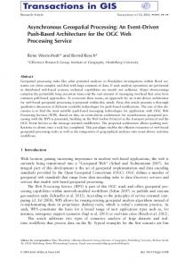
Figure 4.1: Screen shot of DBpedia page describing a River, showing the quantitative and qualitative spatial attributes.

4.3

Geo-spatial Content of DBpedia

In this work, the main interest is the geo-spatial content of DBpedia dataset. In other words, the structured descriptions of geo-spatial places and features such as cities, towns, rivers, and other features or places. In DBpedia, entities or subjects, either geo-spatial or not, are represented uniquely by URIs (Universal Resource Identifier). Every entity is defined as a subject that has properties that in turn have values. These values can be either absolute values such as strings and numbers or they could be other subjects (URIs). Although the DBpedia is a multi-domain dataset, it contains a huge amount of geo-spatial data. Geo-spatial features are geo-referenced in DBpedia either quantitatively or qualitatively. Quantitative attributes of DBpedia objects are described explicitly by the coordinates of the object. They are defined in three ways; first using WGS84 reference system, separating the lat and long of the object; second, using Georss representation combining the lat and long of the object, and third, using the WKT representation POINT(long lat), as shown in figure 4.1. The figure also shows at the top a qualitative attribute of the object, in this case dbprob4 :region, which denotes the location of the object. Geo-spatial content of DBpedia is categorised into non-spatial attributes of a spatial object, spatial properties and spatial relationships.

4

dbprop stands for

56

4.3 Geo-spatial Content of DBpedia

4.3.1

Non-spatial properties in DBpedia

In DBpedia, geographic features are described using spatial and non-spatial properties or attributes. Non-spatial properties are those attributes that are not related to the location of the geographic object. They can be stored in a non-spatial database and queried using SQL. An example of the non-spatial attributes in DBpedia is the population of a city.

4.3.2

Spatial Properties in DBpedia

Spatial properties are those related to the location of the entities in space. They can be classified as quantitative, such as the coordinates of the place, and qualitative such as dbp-ont5 :location, which implies that the specified place or feature is located inside the second place of the predicate. In figure 4.1, the property shown at the top of the figure implies a spatial relationship of containment. In other words, it means that the river described in this DBpedia page is located inside the place on the right side, Derbyshire,Nottinghamshire. In the case of a linear feature such as river the containment property does not mean fully contains but it means overlapping.

4.3.3

Spatial Relation Attributes

In DBpedia every real-world entity is represented as a subject, defined uniquely by a URI such as dbp:Egypt. This subject is characterised using statements that describe facts about it. The statements are organised as triples of . The subject is the real-world object such as Egypt. The predicate is the property describing a feature of that object such as capital. The object is the value assigned to that property such as Cairo, described as being the capital of Egypt. Properties, predicates and attributes are used interchangeably for describing the relationship between the subject of the DBpedia page and the objects or the values. Spatial relation attributes (properties) in DBpedia describe the relationship between two places or geographic features. An example of these spatial attributes is dbp-ont:country, which means that the first argument (subject), which is referred to here as Located Object (LO), is located inside the second one referred to as the Reference Object (RO). The following statement: dbp:Cardiff dbp-ont:country dbpdbp:United_Kingdom is an example of a containment relationship. It means that Cardiff is located inside the United Kingdom. Thus, spatial properties or attributes describe the relationship between a located object (LO) and a reference object (RO). In DBpedia the LO may be the subject of the article or, 5

dbp-ont denotes: http://dbpedia.org/ontology/

4.3 Geo-spatial Content of DBpedia

57

in the case of directional relations, the subject of the article may be the RO. Generally, spatial relations are classified into three categories - topological, proximity and directional.

Topological Topological relations describe the equality, overlapping, crossing and containment between spatial objects. All topological relations between simple regions are defined in the 9-intersection model defined by Egenhofer et al.[53]. Topological relationships are defined in OGC[7] and current GIS extensions of DBMS, such as PostGIS, provide operators to calculate topological relations such as ST_contains, ST_crosses and ST_overlaps. To compute these relations geometrically the existence of the detailed geometry is essential. In DBpedia, there are qualitative predicates that imply containment spatial relations between geo-spatial regions. Some of these predicates are presented in Tables [ 4.1 and 4.2]. They are categorised by the subject place type. The predicates in the table were obtained from an experiment using 20 different regions having geographic boundaries. For each region SPARQL queries were used to retrieve all the relationships (predicates) between the region and each of a set of place types as listed in Tables [ 4.1 and 4.2]. The place types were identified by using spatial database queries to find all DBpedia geo-referenced objects that lay inside the polygonal boundaries of the 20 selected regions. The boundaries were obtained from Ordnance Survey digital map data. It is noted that for the linear features such as rivers the containment predicates are representing partial containment, not full containment.

Proximity or metric Proximity relations are those involving distances. In DBpedia predicates, there are some predicates that imply proximity relations qualitatively, such as dbprop:nearN, dbprop:nearE, dbprop:nearS, dbprop:nearW, dbp-ont:nearestCity and dbp-ont:nearestTown. These predicates are supposed to mean near, but the statistical analysis of these predicates revealed that they are used inconsistently. Figure 4.2 shows the histograms of distances between ROs and LOs for the DBpedia predicates dbprop:nearN, dbprop:nearE, dbprop:nearS, dbprop:nearW. It is noted that the resulting average distances between RO(s) and LO(s) of near predicates are very big about 500-1500 KM - which does not seem to be a sensible distance between places that are supposedly close in proximity. Thus, they can not be used as interpretation of near and have not been used in query processing described in later chapters.

58

4.3 Geo-spatial Content of DBpedia

Directional These properties describe the direction between a LO and a RO. The four basic cardinal directions are north, south, east and west. There are four additional directional relationships northeast, northwest, southeast and southwest. An example of these spatial attributes in DBpedia is north, which means that the second argument(s) or object(s) is/are north of the first one (subject). Examples of spatial directional properties in DBpedia for Cardiff are presented in Table 4.3. There is no standard method for calculating spatial directional relations. They are not supported in current DBMS with spatial extensions. Thus, in this work, a method for quantifying and querying these predicates on the Semantic Web is presented in the next section.

Figure 4.2: Distance histograms for distances between LOs and ROs for predicates implying proximity nearN, nearS, nearE and nearW.

Representing spatial directional relations An interesting area of research in Geographic Information Science is studying people’s perceptions of spatial objects and spatial relations between them and modelling their usage of spatial

4.3 Geo-spatial Content of DBpedia

59

relations. Spatial relations have been studied in many research areas such as cognitive science, linguistics and psychology[65]. A spatial directional relation involves located object(LO) and a reference object (RO). A frame of reference which specifies the context of the relationship is essential.

Class

Property

Meaning

Airport

dbp:location

Location containing the airport

Airport

dbp-ont:location

Location containing the airport

Airport

dbp-ont:city

City containing the airport

Canal

dbp-ont:startPoint

The location of the start of the canal

Canal

dbp-ont:endPoint

The location of the end of the canal

Canal

dbp:shireDistrict

District containing the canal

Canal

dbp-ont:district

District containing the canal

Church

dbp:location

Location containing the Church

Church

dbp-ont:location

Location containing the Church

Church

dbp:address

Address of place containing the Church

Church

dbp-ont:principalArea

Location of area containing the Church

Church

dbp-ont:ceremonialCounty

County containing the Church

Church

dbp:lieutenancyEngland

Location containing the Church

Church

dbp:locationTown

Town containing the Church

Church

dbp:parish

Parish containing the Church

Hospital

dbp-ont:state

State containing the Church

Hospital

dbp-ont:region

Region containing the Church

Hospital

dbp-ont:location

Location containing the hospital

Hospital

dbp:location

Location containing the hospital

Hospital

dbp:parish

Parish containing the hospital

Hospital

dbp:region

Region containing the hospital

Table 4.1: Per class Properties that imply containment in DBpedia.

60

4.3 Geo-spatial Content of DBpedia

Class

Property

Meaning

Hotel

dbp:location

Location containing the hotel

Hotel

dbp-ont:location

Location containing the hotel

Hotel

dbp:locationTown

Town containing the hotel

Island

dbp-ont:ceremonialCounty

County containing the island

Museum

dbp-ont:location

Location containing the Museum

Museum

dbp:location

Location containing the Museum

Park

dbp:location

Location containing the Park

Park

dbp-ont:location

Location containing the Park

Restaurant

dbp:city

City containing the Restaurant

River

dbp:region

Region containing the river

River

dbp:sourceRegion

Region source of the river

River

dbp-ont:sourceRegion

Region source of the river

River

dbp-ont:region

Region source of the river

River

dbp:city

City the river passing through

River

dbp-ont:city

City the river passing through

River

dbp-ont:district

District the river passing through

River

dbp:mouthLocation

Location of the mouth river

River

dbp-ont:mouthPlace

Location of the mouth river

River

dbp:county

County the river passing through

River

dbp:sourceLocation

Location of the source river

River

dbp:state

State the river passing through

River

dbp:mouthDistrict

Location of the mouth river

shoppingMall

dbp:location

Location containing the Mall

shoppingMall

dbp-ont:location

Location containing the Mall

Stadium

dbp:location

Location containing the Stadium

Stadium

dbp-ont:location

Location containing the Stadium

Theatre

dbp:locationTown

Town containing the Theatre

Theatre

dbp:city

City containing the Theatre

Theatre

dbp-ont:locationCity

City containing the Theatre

University

dbp:county

Country containing the University

University

dbp:state

State containing the University

University

dbp-ont:state

State containing the University

University

dbp-ont:city

City containing the University

University

dbp:City

City containing the University

University

dbp:Location

Location containing the University

Table 4.2: Per class Properties that imply containment in DBpedia. Cont.

4.3 Geo-spatial Content of DBpedia

Subject

dbpedia:Cardiff

61

property dbpprop:south

Object dbpedia:Penarth dbpedia:Barry,_Vale_of_Glamorgan dbpedia:Dinas_Powys

dbpprop:north

dbpedia:Pontypridd dbpedia:Caerphilly dbpedia:Aberdare dbpedia:Brecon

dbpprop:east dbpprop:west

dbpedia:Bristol_Channel dbpedia:Rhondda dbpedia:Llantrisant

dbpprop:northeast

dbpedia:Newport dbpedia:Chepstow

dbpprop:northwest

dbpedia:Rhondda dbpedia:Llantrisant

dbpprop:southeast dbpprop:southwest

Bristol_Channel dbpedia:Cardiff_Airport dbpedia: Llantwit_Major

Table 4.3: Spatial Directional relations in DBpedia for Cardiff.

Directional relations between two objects cannot be expressed separately without a frame of reference. In linguistics, the terms ’ground’ and ’figure’ are used instead of RO and LO [169]. There are three frames of references relative or deictic, intrinsic and absolute frame of reference[169]. In the first frame of reference, the spatial relation definition (specification) relies on the orientation and location of the observer and locations of both the reference and located objects such as at the left of the house. The second frame of reference is the intrinsic in which the spatial relation is specified by the orientation of the reference and the locations of the reference and located objects, e.g. at the front of the house. The

62

4.4 Evaluating the positional accuracy of DBpedia data points versus OS

absolute frame of reference is used to specify the spatial relations in DBpedia. In this frame, the spatial relationship is fully defined by the located object (LO) and the reference object(s) only, e.g to the north of the house. In the literature, dealing with spatial directional relations is performed with two methods. The first is transforming it into a quantitative model such as Hall et al.[77], or treating it in a qualitative way and using qualitative spatial reasoning techniques such as Frank et al.[61]. The analysis of the directional relations in this thesis is similar to that of Hall et al.[77], who performed a quantitative analysis for the spatial prepositions for image captions based on multiple instances of realworld use of individual spatial relations. They created quantitative models of spatial directional relations for qualitative spatial directional relations of image captions. They also found that in the context of photo captioning the distances between located (LO) and reference (RO) objects are always small, mostly less than 3000 metres.

4.4

Evaluating the positional accuracy of DBpedia data points versus OS Min

Max

Avg

STD

Mean

1.06014E-05

9.091814935

0.124409556

0.674091757

0.00583069

Table 4.4: Descriptive statistics showing the distance in kilometres between DBpedia points and OS points.

As DBpedia is the main Semantic Web dataset used in this thesis, it is important to evaluate the quality of DBpedia points. Positional accuracy as described in Chapter 2 evaluates the accuracy of the location of the geo-spatial features. Geo-spatial features in DBpedia are represented quantitatively by point coordinates. In order to assess the positional accuracy of the points in DBpedia, a random set of 500 points from DBpedia for the settlements class has been matched with their equivalent instances of the same class in an Ordnance Survey (OS) dataset described in Chapter 2. Due to the high quality of the OS data, it is assumed in this evaluation that the OS data are correct, when contradicted by other data. There are 330 matched instances and the distance between each pair of instances has been calculated. Finally, a set of descriptive statistics has been used to compare between the same points in DBpedia and in OS. Descriptive statistics presented in Table 4.4 shows that the maximum difference between OS points and DBpedia points in terms of distance is about nine kilometres and the average difference is 0.12 kilometres. Hence, there is strong evidence that DBpedia points data have good quality in terms of the positional accuracy. Thus, the problem in DBpedia is not the point representation, which may be acceptable depending on

4.5 Quantitative Analysis of DBpedia Directional Relations

63

the application, but the fact that the point representation is sometimes abstracting important details about geo-spatial features. This abstract representation is unsuitable for representing geo-spatial features with large extent such as, regions and rivers, as using these to compute spatial relationships may produce misleading results.

4.5 4.5.1

Quantitative Analysis of DBpedia Directional Relations Overview

The data used for analysis are spatial directional predicates extracted from DBpedia, that come originally from the Wikipedia Compass-Table infobox 6 . In this analysis, each directional relation contributed by a Wikipedia editor is regarded as a human perception of a preposition describing directional relations. Wikipedia has given instructions for editors of this compass-table. The editing instructions instruct editors of the table to add places of the same level, and not to mix different types of geographic features. If the editors always obeyed the editing instructions then this would limit the value of the data in that the distance relations might simply reflect typical distances between places of the same type as the subject of the Wikipedia page. In practice, from manual inspection of Wikipedia, it is clear that most of the time, editors do not obey the instructions. For example, in the Cardiff Wikipedia page, there are places asserted as having directional relations with Cardiff from different geographical feature types, i.e. airport. To justify treating these assertions as a cross section of human interpretation of directional relation, a set of 20 Wikipedia pages has been examined manually by inspecting their edit history. We found out that each Wikipedia Compass-table has been edited by between two and 13 editors. We also identified at least 85 different contributors to the Compass-Tables. Thus, these can be safely considered to reflect a range of user interpretation of spatial directional relations. However, there remains uncertainty over the extent to which users have rigidly obeyed the editing instructions.

4.5.2

Purpose

The purpose here is to create quantitative models of the concepts involved in directional relations, such as distances and angles between RO(s) and LO(s). These models of directional relations are subsequently used to interpret and display results of directional relations involved in question answering or search engines. In this thesis the directional relations models are used in answering geographic directional queries. This section provides the details about the investigation of qualitative spatial directional relations in DBpedia. First, it presents the data collection from DBpedia and its cleaning procedure. Then, a data analysis for distance and angles respectively is presented before investigating the relation between the distance and angles using scatter plots. 6

http://en.m.wikipedia.org/wiki/Template:Compass-table

64

4.5.3

4.5 Quantitative Analysis of DBpedia Directional Relations

Data Collection

The data used for this experiment were collected from the publicly available DBpedia SPARQL endpoint [3] for each spatial directional relation (N,S, E, W, NE, NW, SE and SW) separately. A set of about 750 places for each cardinal direction 750*8=6000 RDF predicates were collected from DBpedia associated with the latitude and longitude for the places related to them with a directional relationship. SPARQL queries were used to retrieve each of the eight directional relations from a SPARQL endpoint. The following query is used to retrieve all the instances that have predicates describing cardinal directional relations (N,S, E, W, NE, NW, SE and SW). Only places in the UK were used in this analysis. 1.PREFIX dbp: 2.PREFIX yago: 3.PREFIX dbo: 4.PREFIX db: 5.PREFIX geo: 6.SELECT distinct ?s ?l ?lat ?long ?lat1 ?long1 7.WHERE {?s a dbo:Place. 8.?s dbp:north ?l. 9.?s geo:lat ?lat. 10.?s geo:long ?long. 11.?l geo:lat ?lat1. 12.?l geo:long ?long1. 13.FILTER (?lat ≥ 50.485279-0.48 && ?lat ≤ 59.95279 + 0.3 && ?long ≥ -5.9-0.3 && ?long ≤ 1.586667 + 0.3)} 14.order by asc(?s)

Here, lines 1-5 define the name spaces used in the query. Line 6 specifies the variables to be retrieved in the query results, subject (?s), object (?l), coordinates of subject(?lat, ?long) and coordinates of the object (?lat1, ?long1). Lines 7-12 determine the restrictions applied on the variables. Line 7 specifies the retrieval of instances of class Place. Line 8 restricts the retrieval of places having a specified spatial directional relation, i.e north. Lines 9 and 10 associate ?lat and ?long variables with the subject(s) coordinates whereas lines 11 and 12 associate the ?lat1 and ?long1 variables with the object (l) coordinates. Line 13 filters the results for places in the UK. It is an approximate filter to just retrieve instances in the UK. The last line, 14, is used to arrange the results in an ascending order by the subject name. The query is customized to obtain data for various spatial directional relations, just by changing the property in line 8 to other spatial directional properties such as south, east, west, and so on.

4.5 Quantitative Analysis of DBpedia Directional Relations

4.5.4

65

Data Cleaning and Calculations

After collecting the data using the previous SPARQL query for each directional relation, duplicates were removed. Then, the distance and angle were calculated for each pair using their lat and long. The azimuth angle7 , also called bearing, is calculated using the following formula:

Azimuth = atan2(sin(lon2−lon1)cos(lat2), cos(lat1)sin(lat2)−sin(lat1)cos(lat2)cos(lon2−lon1)) (4.1)

Distance = 6378∗ACOS(COS(Lat1)∗COS(Lat2)∗COS(lon2−lon1)+SIN (Lat1)∗SIN (Lat2)) (4.2) where lat1: latitude of the first point. lon1: longitude of the first point. lat2: latitude of the second point. lon2: longitude of the second point. It is noted that in EXCEL the parameters for atan2 function are reversed. After getting the angles, they are converted to degrees and normalised to the range 0-360 by calculating angle=(angle+360) modulo 360. Then, some inconsistent instances were removed; for example instances that have very big distances. After investigation, these turned out to come from the wrong assignment of lat and long for places. It is worth mentioning that the azimuth angle is calculated forward clockwise from exact north=0, 360.

4.5.5

Data Analysis

After collecting the data from DBpedia SPARQL endpoint [3] and cleaning them, the distances and angles in degrees were calculated between each pair of subject and object obtained. The statistical analysis was carried out using R statistical package8 . The results of the analysis are presented in the following section. 7 8

http://www.movable-type.co.uk/scripts/latlong.html http://www.r-project.org/

66

4.5.6

4.5 Quantitative Analysis of DBpedia Directional Relations

Results

This section provides the results of the quantitative analysis of distances and angles between subjects and objects for each of the DBpedia qualitative spatial directional relations. A summary of statistical results obtained from analysing the distances between pairs of subject and object is presented in Table 4.5. The distance histograms for some of the directional relations are shown in Figures [ 4.3 - 4.8] and the accumulated distance histogram over all the different relations is shown in Figure 4.9. The angle histograms circular plots are shown in Figures [ 4.15 and 4.16]. Rose diagrams for the angles are shown in Figures [ 4.17 and 4.18].

Distance Analysis

Table 4.5 compares the results obtained from the preliminary analysis of distances between RO(s) and LO(s) for each of the spatial directional relations in DBpedia. The mean distance for East relationship is clearly different from the other relations as shown in Figure 4.4. The boxplot for the distances between RO(s) and LO(s) for all the spatial directional predicates are shown in Figure 4.10. There are no significant differences between their medians, but the third quartile is about 12 or 13. So, 75% of subjects are less than about 12.5 KM from their corresponding reference object. Applying Shapiro-Wilk normality test for all the spatial relations, they are not normally distributed which can be seen in the histograms presented in figures[ 4.3 - 4.8]. Further statistical analysis revealed that they do obey a log-normal distribution. What is surprising is that people tend to refer to locations within a small distance - about 10 KM of their location.

Relation

Min

1st Qu

Median

Mean

3rd Qu

Max

North

0.17

2.4

4.2

13.1

9.8

350

South

0.008

2.4

4.4

12.2

10.5

125

East

0.07

2.5

4.3

8.3

9.4

350

West

0.07

2.7

4.7

12.3

13.2

270

Northeast

0.08

3.1

5.3

11.9

15.1

250

Northwest

0.09

3.1

4.9

13.4

13.1

350

Southeast

0.49

3.1

5.5

13.2

13.3

260

Southwest

0.02

3.2

5.3

11.9

13.8

270

Table 4.5: Summary statistics for distances in KM between subject(s) and object(s) for different spatial directional relations.

4.5 Quantitative Analysis of DBpedia Directional Relations

Figure 4.3: Histogram for the distance in KM for North relation.

Figure 4.4: Histogram for the distance in KM for East relation.

67

68

4.5 Quantitative Analysis of DBpedia Directional Relations

Figure 4.5: Histogram for the distance in KM for West relation.

Figure 4.6: Histogram for the distance in KM for Northeast relation.

4.5 Quantitative Analysis of DBpedia Directional Relations

Figure 4.7: Histogram for the distance in KM for Southeast relation.

Figure 4.8: Histogram for the distance in KM for Southwest relation.

69

70

4.5 Quantitative Analysis of DBpedia Directional Relations

Figure 4.9: Histogram for the accumulated distance in KM over all spatial directional relations.

Figure 4.10: Box plot for the distance in KM for all spatial directional relations.

4.5 Quantitative Analysis of DBpedia Directional Relations

71

To show if distances between RO(s) and LO(s) are affected by the place type of the RO the following experiment has been conducted. A collection of pre-classified instances in DBpedia ontology has been acquired to model the city, town and village classes in terms of their population. This resulted in a very low median for city about 4000, 1000 for town and 400 for village. Thus, we re-categorised the places into small places up to 2000, medium places 2000-50000, and bigger places above 50000. Using the new categorization scatter plots have been used to show the relation between the distance and population for different classes. Figures [ 4.12 - 4.14] show the scatter plots for the relationship between population and distance for small places, medium size places and bigger places respectively and Figure 4.11 shows the box plot for the distances between the RO and LO for different place types. It is noted that the mean values are nearly the same, which means that, the distances between the RO and the LO is not affected by the place types.

Figure 4.11: Box plot for the distance in KM for for small, medium and bigger places.

72

4.5 Quantitative Analysis of DBpedia Directional Relations

Figure 4.12: Scatter plot for the relation between population and distances in KM between RO(s) and LO(s) for small places.

Figure 4.13: Scatter plot for the relation between population and distances in KM between RO(s) and LO(s) for medium size places.

4.5 Quantitative Analysis of DBpedia Directional Relations

73

Figure 4.14: Scatter plot for the relation between population and distances in KM between RO(s) and LO(s) for bigger places.

It is apparent from the scatter plots in Figures [ 4.12, 4.13 and 4.14] and the box plot shown in Figure 4.11that the distances recorded between the RO(s) and LO(s) are not affected by the place type. It is surprising that for all classes of places categorised by their corresponding population, the distances between the RO(s) and LO(s) tend to have similar patterns. The regular pattern noted is that different place types have small distances between the RO(s) and LO(s).

Angle Analysis If we now turn to the angle analysis, the conventional statistical methods are not appropriate for the circular data. If we looked at , for example, the mean value for two angles in degrees 0 ◦ and 360 ◦ , the arithmetic mean will be 180 ◦ , which is not sensible value. Thus we apply circular statistics to compute the mean value for each direction. For north of relationship the azimuth angle mean was 350 ◦ , i.e. with a deviation of 10 ◦ towards west. The south of relationship has a mean of 176.6 ◦ , which has a small deviation of 3.4 ◦ to the east. For east of relationship, the mean angle was 89.38 ◦ , which is nearly perfect east. In addition, the west of relationship has a mean of 267.60 ◦ , which has a small shift of 2.4 ◦ towards south. The actual azimuth angles histogram, raw data circular plot, for each relationship is presented in Figure 4.15, for the four basic spatial relations and in Figure 4.16 for the other four intermediate spatial relations.

74

4.5 Quantitative Analysis of DBpedia Directional Relations

Figure 4.15: Circular raw data Plot of the actual angle data for the four basic spatial directional relations (North, South, East and West) in DBpedia.

4.5 Quantitative Analysis of DBpedia Directional Relations

75

Figure 4.16: Circular raw data plots for the actual angle data histograms for the four intermediate spatial directional relations (Northeast, Northwest, Southeast and Southwest).

76

4.5 Quantitative Analysis of DBpedia Directional Relations

Figure 4.17: Rose Diagram for the angles between the subject(s) and object(s) for the basic spatial directional relations (North, South, East and West). Each stack of points on the circle represents the number of points in this direction with the corresponding azimuth angle. These graphs demonstrate the distribution of points around the circle. To create smoothed diagrams which show the intervals for each cone representing the density of points, rose diagrams have been used for all the circular diagrams created in Figures 4.15 and 4.16 above. The rose diagrams for the basic directional relations are presented in Figure 4.17 and for the intermediate spatial directional relations in Figure 4.18. For the intermediate spatial directional relations, the northeast relation has a mean of 47.9 ◦ , which has a little shift of 2.9 ◦ to the east. For northwest, the mean is 305 ◦ , which is also shifted by 10 ◦ towards north. For the southeast relation, the mean of the angle between the subject (s) and objects is 129 ◦ , which is slightly shifted by 6 ◦ to the east. The southwest relation has a mean of 224 ◦ , which has a very small shift of 1 ◦ towards the south. The actual raw data have been plotted as circular plots in Figure 4.16

4.5 Quantitative Analysis of DBpedia Directional Relations

77

Further statistical tests of uniformity distribution of circular data have been conducted for all the directional relations, such as Kuiper test and Watson test at p-value < 0.01. The result was to reject the null hypothesis that the circular data are uniformly distributed around the circle.

Figure 4.18: Rose Diagram for the angles between the subject(s) and object(s) for the intermediate spatial directional relations (Northeast, Northwest, Southeast, and Southwest).

4.5.7

Relationship between Distance and Angle

From this point, the research focuses on the four basic directional relations. In the previous results the distances and the angles between the subject(s) and the corresponding object(s) of DBpedia spatial relation predicates have been quantitatively described and graphed. It is important to turn now to the experimental evidence that shows the relationship between the angles and distances for each directional relationship. The scatter plots in Figures [ 4.20, 4.22, 4.24 and 4.26] show the relationship between the angles and distances for each of the four basic directional relationships using simple scatter plots. While,

78

4.5 Quantitative Analysis of DBpedia Directional Relations

Figures [ 4.19, 4.21, 4.23 and 4.25] show the high density scatter plots representing the relation between the angles and distances for the four basic directional relations. Generally, it can be noticed that as the distance increases the number of points satisfying the spatial relation decreases. It can be concluded that there is an inverse relationship between the distance between the RO and LO and the assignment of spatial directional relations.

North From figure 4.20 the scatter plot for north relationship, the points have an angular range between (0 ◦ 90 ◦ ) and (270 ◦ - 360 ◦ ). The highest density ranges of the points are (0 ◦ - 22.5 ◦ ) and (337.5 ◦ - 360 ◦ ). The density of points declined from (22.5 ◦ to 90 ◦ ) and from (337.5 ◦ to 270 ◦ ). It is apparent in this figure that the density is decreasing in accordance with the distance. Higher densities are concentrated within a distance of (0-10) KM.

South From figure 4.22 showing the scatter plot for south relationship, it is apparent that the range of the angles is (90 ◦ - 270 ◦ ) . The highest density is recorded at the range (157.5 ◦ - 202.5 ◦ ). The density of the points is decreasing in both directions from (157.5 ◦ ) downwards and from (202.5 ◦ ) onwards. The figure also reveals that the density is decreasing as the distance decreases, recording highest densities at distance range (0-10) KM.

East Figure 4.24 showing the scatter plot for east relationship indicates that the angle range is (0 ◦ - 180 ◦ ). The highest density for this relation has been recorded at the range (76.5 ◦ - 112.5 ◦ ). There is a clear trend of decreasing in the density from (76.5 ◦ ) downwards and from (112.5 ◦ ) onwards. The same trend is recorded for distances as noted in the previous relations of decreasing the density with the distance increase, with the highest density at (0-10)KM.

West Figure 4.26 shows the scatter plot for the west relationship, within the angular range of (180 ◦ - 360 ◦ ). The highest densities of the points are (247.5 ◦ - 292.5 ◦ ). The density is decreasing in both directions from (247.5 ◦ ) downwards and from (292.5 ◦ ) onwards. There is a decrease detected in the density of points associated with the distance increase. The points having the highest densities are within the range (0-10) KM.

4.5 Quantitative Analysis of DBpedia Directional Relations

79

Figure 4.19: Scatter plot for the distance and angle between object and subject(s) for North relationship.

Figure 4.20: Scatter density plot for the distance and angle between object and subject(s) for North relationship.

80

4.5 Quantitative Analysis of DBpedia Directional Relations

Figure 4.21: Scatter plot for the distance and angle between object and subject(s) for South relationship.

Figure 4.22: Scatter density plot for the distance and angle between object and subject(s) for South relationship.

4.5 Quantitative Analysis of DBpedia Directional Relations

81

Figure 4.23: Scatter plot for the distance and angle between object and subject(s) for East relationship.

Figure 4.24: Scatter density plot for the distance and angle between object and subject(s) for East relationship.

82

4.5 Quantitative Analysis of DBpedia Directional Relations

Figure 4.25: Scatter plot for the distance and angle between object and subject(s) for West relationship.

Figure 4.26: Scatter density plot for the distance and angle between object and subject(s) for West relationship.

To conclude, It can be noted that there is specific angle ranges with higher point densities, such as the centre of each direction of North, South, East and West directions. Meanwhile, the point density is

4.6 Summary

83

decreasing while increasing the distance for all the specified directions.

Discussion From the previous analysis it can be concluded that there are clear patterns of point densities around specified angle ranges for each of the basic directional relationships. Moreover, there is a general trend of decreasing in the point densities associated with increasing the distance. lm.circular is a function in circular9 R package. This function finds a regression model fit for either a circular-circular which finds a model for a circular-dependent and a circular-independent variable or a circular-linear which finds a model for a circular-dependent and a linear-independent variable. Using the circular-linear function with the angle variable as a circular dependent variable and the distance as a linear-independent variable, no good fit for a mathematical model of the relationship between distances and angles was identified using the circular statistics model fitting. This might be due to the small sample size in the dataset. However, it is important to find a method to use the results in processing directional geo-spatial queries. Thus, we propose a method to use the weight for each of the variables distance and angle to rank the results of the directional relationship queries based on these empirical facts. The proposed ranking method is to give a weight for each retrieved point on the basis of its angle, which is given by the density in the angle range containing the point, and its distance weight is the inverse of the distance, as was indicated from the analysis that the density is decreasing as the distance increase. The final weight for the point is angle weight/distance weight. The method is explained in more details in Section 5.3.7. This weight is used to rank the results of the query. There was no evidence that the distances and angles between RO(s) and LO(s) are affected by the type of RO.

4.6

Summary

This chapter began with an introduction to the DBpedia dataset, followed by a discussion of various DBpedia access methods, emphasising that SPARQL endpoint is the method of choice in this thesis for data collection. Then it presented a description of various geo-spatial contents of DBpedia, including nonspatial properties, spatial properties and spatial relation attributes. Concerning spatial relations, various spatial relations have been discussed including topological relations, supported by a list of spatial containment properties extracted from DBpedia, proximity relations and directional relations. A particular attention has been paid to directional relations as it is the core subject of the discussion in the rest of the chapter. This was followed by an evaluation of the positional accuracy of geographic feature points against OS geographic detailed feature representation. Finally, the focus shifted to the investigation of quantifying qualitative spatial directional relations in 9

http://cran.r-project.org/web/packages/circular/circular.pdf

84

4.6 Summary

DBpedia, which were extracted from Wikipedia user contributions. The quantitative analysis of DBpedia spatial directional relations began with an overview of the main source of the prepositions describing directional relations (Wikipedia compass-table), then stating the purpose of the analysis. Following this, the data collection procedure was discussed, followed by data cleaning and mathematical calculation of the azimuth angle. This is followed by the statistical analysis procedures for the two variables, azimuth angles and distances between subject(s) and object(s), of DBpedia directional predicates, referred to here as LO(s) and RO(s). This is then followed by showing the results of the analysis. Beginning with the analysis of distance, a statistical summary showed that the east relationship has the smallest mean value. Boxplots showed a comparison between different spatial directional relations, in terms of mean values and quartile ranges, showing that there is no significant difference between distances in all eight spatial directional relations. Then the discussion shifted to the analysis of the angles, describing the statistical circular mean value for each directional relation. Beside this, angular data exploration involved using circular plots to show the distribution of the angles in various spatial directional relations. Similarly, rose diagrams were used to show the intervals of density of points for angle ranges for different relations. Further statistical methods have been investigated to test the distribution normality of angles around the circle. Finally, the relationship between the distances, angles and density of points was used to investigate the possibility of finding a mathematical formula to be used to model the relationship between angle and distance pair. This resulted in finding no suitable fit for a mathematical model. Thus, a method depending on the weight combining the distance and angle has been proposed to be used in the processing of spatial directional questions. The next chapter presents the analysis and design of the system prototype that enables answering geo-spatial questions with spatial relationship restrictions.

85

Chapter 5

System Analysis and Design

5.1

Introduction

This chapter presents the analysis and design stages of building a prototype for a query answering system, to support the answering of geo-spatial questions, particularly ones with spatial relation constraints. It includes the functional requirements of the proposed prototype of a question answering system. The presented design includes the system architecture, database design, query planner design and user interface design.

5.2

System Analysis

The classical approach for building an information system incorporates three main stages, analysis, design and implementation. System analysis is the process involving collecting information and facts about the current situation of a system either by testing or investigations of an existing system, to identify problems and recommend requirements for a solution or improvements.

5.2.1

Requirements Analysis - Problem Statement

As indicated in the literature review, the limitations of existing GQAS can be summarised in two points: first, the inability to answer geo-spatial questions with spatial relation constraints. Second, the utilisation of only textual or web search engine results or websites for answering geo-spatial questions, thus, limiting its ability to answer questions that require geo-spatial computations. Consequently, the functionalities requirements of the proposed system are: First, the system should support users for answering geo-spatial questions, particularly those with spatial relationships. Geo-spatial questions can be classified into the following categories: 1. Non-spatial attribute questions. 2. Spatial attribute questions.

86

5.3 System Design 3. Spatial relationship questions. • Topological (Containment/ Crossing). • Proximity. • Directional.

Second, the system should utilise the new emerging Semantic Web data sources, namely DBpedia, for answering geo-spatial questions associated with higher-quality geo-data (OS) to improve the geo-spatial query answering. It should also combine the quantitative and qualitative attributes in the question answering process. Figure 5.1 shows a high-level sequence diagram for the system operations. The diagram shows the sequence of operations for answering geo-spatial questions of the types specified in the requirements analysis. Initially, the user formulates the question through the user interface. Then, according to the question parameters given and the type of question, a specific query plan is executed by the query processor. The query plan is an ordered set of one query or a number of queries to data sources to answer a question. Then, the results of the queries are combined and presented and could be associated with a map to show the locations of the objects.

Figure 5.1: Query Answering System Sequence Diagram.

5.3

System Design

This section provides the design of different components of the proposed query answering system, in particular, the system architecture, the database design, and the design of various query plans for answering different types of geo-spatial questions, and finally the design of the user interface.

5.3 System Design

5.3.1

87

System Architecture

The query answering system consists of a set of components (see figure 5.2). The user interface enables the user to formulate and disambiguate the place or geographic feature name in the questions. The place name disambiguation is embedded in the question formulation process. The query processor is responsible for processing questions received from the user interface and executing the appropriate query plan according to the question type, determined by the query planner. Data sources are partially locally stored, as in the Dbpedia index, which is composed of geo-spatial features and their corresponding locations from DBpedia and OS geo-data, which contain detailed geometric representation of geo-spatial features such as region boundaries. The geo-feature links are links between features from DBpedia and their corresponding features in OS geo-data, which are essential for combining quantitative and qualitative properties in answering containment questions. DBpedia data can also be remotely accessed, providing online access to DBpedia contents when required. More details on the actual implementation of the system are provided in the next chapter.

Figure 5.2: System Architecture.

88

5.3.2

5.3 System Design

Database Design

The data sources for this system are DBpedia data and OS detailed geo-data. For each data source a different table schema has been designed. The design of the DBpedia data table is shown in Figure 5.3. This table contains ID, as a primary key; URI, which is the identifier for each DBpedia entity; lat is the latitude of the DBpedia entity; lon is the longitude of the DBpedia entity; the_geom and geom are the geometric point representation of the location of the entity, composed of combining lon and lat, in the WGS84 and OS British National Grid reference system respectively; and finally the name of the entity created from the URI of the entity. The schema of the OS data table is shown in Figure 5.4 showing the name of the entity and its detailed geometry in the British National Grid reference system. The database table schema for links between both datasets is shown in Figure 5.5, where each DBpedia entity is linked with the corresponding entity in OS geo-data.

Figure 5.3: Database table design for the DBpedia data.

Figure 5.4: Database table design for the Ordnance Survey data.

Figure 5.5: Database table design for links between the DBpedia data and the OS geo-data.

5.3 System Design

5.3.3

89

Query planner design

This section provides descriptions of different query plans, used for various question types. Question types are either spatial or non-spatial. Non-spatial questions are those asking for a non-spatial property not related to the location of the place or feature, such as population. Spatial questions can be classified into spatial attribute questions and spatial relation questions. Spatial attribute questions are asking directly about the location of a specific place or feature, such as Where is Cardiff_ Airport? Spatial relation questions can be categorised into topological, proximity or metric and directional. Topological questions are related to the topology of the spatial relation such as containment, crossing and overlapping. An example of a topological question is Find hospitals inside Cardiff? Proximity questions are those associated with distance; for example, Find hospitals within 10 KM of Cardiff? Finally, the directional questions are those related to the cardinal directions, for example, Find hospitals north of Cardiff? In the following sections the query plans for these types of questions are presented and discussed.

5.3.4

Non-spatial questions query plan

This query plan is performed to answer questions asking for non-spatial properties, such as What is the capital of Wales? For the system to answer this type of question, it performs the following steps. First, the disambiguated geo-spatial place or feature name is obtained from the user interface such as "Wales", and the name of the required property, such as "Capital". Then, a SPARQL query is formulated with this property and sent to the SPARQL endpoint. The answer returned is then presented to the user. This query plan is described in Figure 5.6.

Figure 5.6: Activity diagram for non-spatial questions query plan.

90

5.3.5

5.3 System Design

Spatial questions query plan

This plan is executed when the asked question is directly related to the location of the place or feature. For example, Where is Cardiff_ Castle? For the system to answer this type of question, it has to implement the following steps. First, the place or feature disambiguated name is obtained from the user interface. Then a SQL query is executed locally to get the lat and long of the place/feature. This is followed by formulation of a SPARQL query asking for the DBpedia page abstract, which is sent to an online SPARQL query endpoint. Finally, the DBpedia page abstract is displayed to the user in association with a map showing the location of the place/feature. The query plan is shown in Figure 5.7.

Figure 5.7: Activity diagram for spatial questions query plan.

5.3.6

Containment questions query plan

This query plan is triggered by a containment question, such as find hospitals inside Cardiff? It is hybrid in the sense that it uses both the polygonal boundary of the RO, if available, and qualitative containment properties if they are present. In order to answer this type of question the system has to perform a series of steps. First, it has to check whether the RO "Cardiff" has detailed geometry or boundary. If it has a polygonal representation, then this representation is considered the query foot-print for the containment query. Then, it has to formulate a containment query to search the instances LO(s) of the specific class, hospital, defined in the user interface inside the RO. Meanwhile, a SPARQL query is sent to a DBpedia SPARQL endpoint to find out if there are any instances from spatial qualitative containment properties

5.3 System Design

91

listed in Chapter 4, describing the RO as containing instances of the class specified in the user interface. Finally, the results obtained are combined, with duplicates removed, and are presented to the user as as a list which can be shown on a map. If the RO has no detailed geometry, the SPARQL query can be still used to retrieve objects that are associated with the RO by a spatial containment property. The query plan is shown in figure 5.8.

Figure 5.8: Activity diagram for containment questions query plan.

5.3.7

Directional questions query plan

This query plan is triggered by a directional question, such as find hospitals north of Cardiff? If the RO has detailed geometry, then this representation is the query foot-print. A SQL query is formulated and executed to calculate its centroid. In the absence of the polygonal representation for the RO, the point representation of the RO is used. Then a SQL query is formulated and executed to find all the instances of the class specified in the user interface in the specified direction, by retrieving the instances in the acceptance region. The acceptance regions for all the spatial relations are shown in Figures[ 5.10 - 5.13]. The query is executed using an initial distance threshold buffer of 15 KM based on the empirical evidence that users are usually referring to places within about 10 KM from the RO, from the distance analysis of the directional relations in Chapter 4. The buffer can be automatically increased by 5 KM if no results

92

5.3 System Design

are obtained. After that, the distance and angle between the RO and each LO are calculated the same as described in Chapter 4 and stored. Using these values, each retrieved instance is given a weight. The weight is computed by angle weight/distance. The angle weight is based on the density of points in the angle range as follows: if angle_in_cones_1_or_2 n then

angle_weight = 100 else ifnangle_in_cones_3_or_4 then

angle_weight = 75 else ifnangle_in_cones_5_or_6 then

angle_weight = 50 else ifnangle_is_in_cone_7_or_8 then

angle_weight = 25

Figure 5.9: Activity diagram for the directional questions query plan.

5.3 System Design

Figure 5.10: Acceptance and rejection regions for north relation.

Figure 5.11: Acceptance and rejection regions for south relation.

93

94

5.3 System Design

Figure 5.12: Acceptance and rejection regions for east relation.

Figure 5.13: Acceptance and rejection regions for west relation.

This is followed by giving each instance retrieved a rank from 1 to 4. The ranking is based on angle weight/distance in KM referred to as weight. Finally, the results obtained are presented to the user and can be shown on a map. The query plan for the directional questions is shown in Figure 5.9.

5.3 System Design

95

if weight n >= 10 then

Rank_instance_1 else ifn7.5 =< weight < 10

then

Rank_instance_2 else ifn5 =< weight < 7.5 then

Rank_instance_3 else ifnweight < 5 then

5.3.8

Rank_instance_4

Crossing questions query plan

This type of question asks about a property for instances satisfying a spatial crossing constraint. It requires data from DBpedia and the detailed geo-data to answer the question. This plan is executed when the asked question is of type crossing, for example Find rivermouth property of rivers crossing Cardiff? For the system to answer this type of question, it has to carry out the following steps. First, it has to consult the geo-data, to see if the RO has detailed geometry and the LO class has detailed geometry such as rivers. If they have, then the query foot-print is used to find rivers crossing Cardiff, with a SQL crossing query. The URIs of the retrieved rivers are used in formulating a SPARQL query to get the property from the DBpedia endpoint. If there are multiple rivers, each property will be retrieved from the DBpedia endpoint. Then the results are represented to the user. The query plan is shown in Figure 5.14.

Figure 5.14: Activity diagram for query plan for crossing queries.

96

5.3.9

5.3 System Design

Proximity questions query plan

Proximity questions are those involving distances, for example Find hotels within 10 KM of Cardiff? For this type of question to be answered, the system will take the following steps. First, it checks whether the RO, which is "Cardiff" in this case, has polygonal detailed geometry. If it has geometry the question can be answered in two ways, either from the centroid in which case places inside Cardiff will be included, or by calculating the distance from the boundary. If the detailed geometry is not present then the point will be used. After getting the geometry, either a point or a polygon, a SQL within distance query is formulated and executed. This query will search the DBpedia index for instances of the specific class specified in the user interface and within the distance specified by the user, from a RO determined by the user and disambiguated throughout the user interface. Finally, the results are presented to the user and can be displayed on a map. Figure 5.15 shows the query plan for proximity questions.

Figure 5.15: Activity diagram for query plan for proximity queries.

5.4 Summary

5.3.10

97

User Interface Design

The user interface is a structured user interface, composed of structured components such as combo boxes and text boxes, where the user can ask structured questions. The interface provides the ability to ask different types of questions such as Non-spatial, Spatial, Proximity, Containment and Directional questions. The interface contains, from the left, a combo box which helps identify the class of the LO. The second combo box specifies the property which changes according to the class of the RO, if the question asks about a property. The third combo box helps to specify the spatial relationship (north, south, east, west, proximity, inside and crossing). The fourth combo box specifies the RO class. The text box helps disambiguate the RO name from a list generated. When the ASK button is clicked the question asked is printed for the user. if the YES button is clicked, the corresponding query plan will be executed. Otherwise, if the NO button is clicked the user will be asked to reformulate the question. The blank text areas are used to display the results. A snapshot of the user interface is shown in Figure 5.16.

Figure 5.16: User interface design.

5.4

Summary

This chapter presented the requirements analysis of the proposed query answering system such as using the semantic web resources for answering geo-spatial questions and supporting various types of geo-spatial questions such as Non-spatial, Spatial, Containment, Proximity, Crossing and Directional questions. Then it provided a description of the design specifications of the proposed system including the system architecture, database schema design, query planner design and the user interface design. The next chapter describes the system prototype implementation details.

98

5.4 Summary

99

Chapter 6

Implementation

6.1

Introduction

The previous chapter discussed the system requirements analysis and system design specifications. This chapter is concerned with the implementation of the question answering system prototype. The implementation phase is the actual coding of the software program, specified in the requirements analysis and described by the system design specifications. In the context of this work the implementation involves the data collection, storage and indexing, the development of query processing for various question types and implementing the user interface and various query plans for different types of questions such as Nonspatial, Spatial, Containment, Proximity, Crossing and Directional. This chapter is organised as follows: it starts with a discussion of the implementation methodology, then presents an overview of the implementation structure, followed by data collection, storage and indexing for both DBpedia data and OS geo-data and creating links between them. Then, the visual user interface implementation is discussed, along with the pseudo code for the implemented modules such as depicting user actions, query planner and detailed query processing steps for different question types.

6.2

Implementation Methodology

The purpose of the system implementation is to demonstrate the feasibility of the proposed methods. An iterative refinement approach has been utilised in implementing the proposed system prototype. In this approach, the desired solution is reached by gradually improving on the initial prototype. The final system architecture was defined previously in Chapter 5. To implement the geo-spatial question answering system prototype, a set of tasks need to be accomplished. The first task is the collection of data from different data sources, storage, indexing and linking the same objects in different data sources (record linkage or entity matching). The second task is to implement the various query plans. The final task is implementing the user interface providing the user with the ability to ask various types of geo-spatial questions.

100

6.3

6.3 Implementation Overview

Implementation Overview

Figure 6.1: Implementation Overview.

The first phase in system implementation is data collection, storage and indexing. The geo-spatial data used in the system are stored in a PostGIS spatial database which contains spatially indexed geo-spatial DBpedia data and OS high-quality geo-data with links between the two sources. The procedure for creating the DBpedia index and linking it with detailed geometry data is presented in the next section. The implementation architecture in Figure 6.1 is composed of three main components. The first component from the bottom is the data access layer, which facilitates spatial SQL queries over the spatial database using PostgreSQL JDBC driver. It also includes the Jena Semantic Web API, which enables the interaction between the system and DBpedia RDF predicates using SPARQL queries. The second component is the query processing component which is responsible for generating query foot-prints from detailed geo-data, formulating spatial SQL queries, such as Containment, Proximity and Crossing or SPARQL queries and executing a specific query plan, formatting the result sets and presenting the results in a suitable format. The last component in the architecture is the user interface. The interface is a crucial component in the system as it enables the user to formulate and pose a question and display the answer back to the user. The user interface is built as a graphical user interface(GUI) using Java swing components such as comboboxes, textboxes and buttons. The following tools have been utilised in the system

6.4 Spatially indexing DBpedia

101

implementation: NetBeans 6.8 IDE is a cross-platform Integrated Development Environment which supports developing applications of various types such as desktop or web applications. It also supports multiple programming languages such as Java, C and C++. It has been used for implementing the prototype. PostgreSQL Database engine is an open source DBMS. It has been chosen for many reasons including the facts that it is a free and open source DBMS and it has spatial extensions (PostGIS) that are used to create the spatial index of DBpedia. It provides built- in string manipulation, fuzzy string similarity functions such as Levenshtein, Soundex and also supports coordinate similarity functions such as Hausdorff distance similarity. There are many DBMS providing spatial extensions such as SQL Server and Oracle. PostgreSQL, in addition to providing spatial extensions, supports built-in similarity functions and coordinate conversion. PostGIS is a spatial extension of PostgreSQL DBMS. It is used to store geo-spatial information and perform spatial SQL queries. Jena is a Semantic Web API that is used to connect the system online with the Virtuoso SPARQL endpoint of DBpedia, to perform SPARQL queries on the fly, without the need to store all the data in a database, which would be an overhead and could increase system response time. Google Maps API is an API used to show the location of answers on a map. PostGIS shapefile and DBF Loader is a software tool that supports the import of shape files into PostgreSQL. Virtuso SPARQL Query endpoint is an online server, providing access to DBpedia RDF contents. It can be accessed in a web browser to query DBpedia or it can be accessed within a program using a Semantic Web API such as Jena.

6.4

Spatially indexing DBpedia

In the proposed system there are two data sources, the Semantic Web dataset (DBpedia) and the higher quality geo-data (OS). The first step in the development of an application is the data collection and storage. In this section, the process of collecting, storing and indexing geo-spatial contents of DBpedia and OS geo-data is discussed.

Data Collection, Storage and Indexing The data collection and storage from DBpedia was performed as follows: • Execute a set of SPARQL queries over DBpedia SPARQL endpoint shown in Figure 6.2, where the SPARQL query is formulated and the required results format is chosen from a set of available options (HTML, Spreadsheet, XML, JSON, Javascript, NTriples, RDF/XML, CSV and TSV). In

102

6.4 Spatially indexing DBpedia this implementation system the CSV1 format has been chosen. Thus, the results of the query are stored as a CSV file, which can then be transformed to a database table schema, specified in Chapter 5. Initially, the table contains the URI, lat and long for each instance. Then the_geom column is obtained by generating a point from each long and lat pair. The the_geom column is a geometry data type in the geodetic format. It is then transformed to the local Great Britain georeference system, to be compatible with the geo-data from OS, thus avoiding the inclusion of these transformation processes in the query processing which affects the speed of the query execution. Then, the name column is constructed from the URI using text processing functions available in the PostgreSQL DBMS. These functions can be used to transform any format of coordinates to long:lat pairs format. The reference system transformation functions are available in PostGIS. For international coverage of the system, it would be possible to use the Geography data type, supported in PostGIS 1.5, which uses geodetic coordinates directly. Although it is less accurate in terms of calculating distances, it is useful for representing geo-data globally rather than for specific regions which require specific reference systems. • SPARQL queries retrieve all instances of a particular class. The classes of features are mainly chosen from DBpedia ontology super-class Place. From the Place class hierarchy, a set of 17 representative sub-classes has been chosen for the experiments. Those classes are shown in Table 6.1 with their corresponding number of instances. The DBpedia ontology is used to identify classes as it has a predefined hierarchy for all its classes and sub-classes. On the other hand, the Yago ontology does not have a clear hierarchy for DBpedia classes. Thus, to specify the equivalent classes of the Yago ontology, a set of instances retrieved from DBpedia ontology with a predefined class has been used to infer the equivalent classes in Yago ontology. The inference mechanism provided in SPARQL makes it possible to traverse the hierarchy to search for sub-classes and sub-sub classes to get all the available instances in parent classes and all their child sub-classes.

The data are stored in a spatial database with spatial indexes created using the_geom and geom columns with the gist PostGIS access method. Note: to carry out spatial operations the data must be stored in the same spatial reference system. The following is a SPARQL query to retrieve all instances from DBpedia ontology and Yago ontology for the Canal class.

1

Comma-Separated Values file format

6.4 Spatially indexing DBpedia

103

1.define input:inference“http://dbpedia.org/resource/inference/rules/ yago#” 2.PREFIX geo:



3.PREFIX dbp-ont:



4.PREFIX grs: 5.SELECT distinct ?s ?lat ?long ?geom ?point 6.

WHERE {

7.

{?s a }

8.UNION 9.{?s a 10.} 11.UNION 12.{?s a ?t. 13.?t rdfs:subClassOf } 14.{?s geo:lat ?lat .} 15.{?s geo:long ?long.

}

16.

OPTIONAL { ?s geo:lat ?lat}

17.

OPTIONAL { ?s geo:long ?lon}

18.

OPTIONAL { ?s geo:geometry ?geom}

19.

OPTIONAL { ?s grs:point ?point}

20.FILTER (?lat ≥ 50.485279-0.48 && ?lat ≤ 59.95279+0.3 && ?long ≥ -5.9-0.3 && ?long ≤ 1.586667+0.3) }

where Line 1 defines the inference rules used to get all instances of sub-classes of the Yago ontology in SPARQL queries. Lines 2-4 specifies the namespaces used in the query. Line 5 determines the variables to be retrieved by the query. Line 7 specifies the DBpedia ontology class to be searched for. Line 8 the UNION keyword is used to integrate the results of multiple patterns to be included in the results. Lines 9 and 10 determine the equivalent class in the Yago ontology to the DBpedia ontology class specified in line 7. Similarly, lines 12 and 13 are used to specify the corresponding subclass of the Yago ontology class. Lines 14-19 retrieve all instances having any type of coordinates. Line 20 approximately confines the search results for instances in the UK region. Similarly, the instances of other classes have been collected from the DBpedia endpoint.

104

6.4 Spatially indexing DBpedia Class

No of instances

Airport

2085

Canal

128

Church

2411

Hospital

453

Hotel

347

Island

820

Lake

515

Mountain

993

Museum

949

Park

617

Restaurant

59

River

700

Shopping Mall

168

Stadium

481

Theatre

439

University

360

Settlement

17558

Table 6.1: Per class number of instances in the DBpedia index.

Figure 6.2: Snapshot of Virtuoso DBpedia SPARQL Endpoint.

6.7 Implementing the user interface and query plans

6.5

105

Storing OS high quality mapping geo-data

Ordnance Survey (OS) detailed geo-data are obtained from the OS mapping agency. The datasets utilised are Meridian 2, Strategi, Boundary-Line and OS VectorMap District data sets. These datasets contain point data for settlements and boundary data for districts, parishes and counties represented as polygons, in addition to rivers represented as lines and lakes represented as polygons. These datasets are supplied from OS as shape files, which cannot be stored into a database directly. Thus, to store these files into a spatial database, shape file and DBF loader plugin for PostGIS has been used.

6.6

Linking DBpedia spatially-indexed data with OS geo-data

Linking similar entities in two datasets in a database is called record linkage or entity resolution or matching. Matching similar geographic features can be performed using various methods, such as name matching methods [41] and coordinate similarity measures such as Hausdorff distance similarity measures as utilised in [157]. Name matching can be performed by either exact matching using the ilike operator, where i refers to ignoring the case or fuzzy string matching. There is a set of fuzzy string similarity matching functions in PostgreSQL, including Levenshtein distance similarity and Soundex functions. In this work, some experimentation was done with using these fuzzy matching functions but when evaluated they resulted in a large number of false positive links. In alleviate this problem, a simpler strategy was adopted whereby, after removing some unnecessary keywords such as river (as the instances are pre-classified), an exact match was applied to the names. The resulting matches were then filtered to eliminate pairs of instances that were more than 20Km apart in their geographic distance. Thus, to minimise the number of false positives, only exact matching only has been used. There is a general rule in QAS that "No answer is better than the wrong answer"[37]. This rule has been applied in this case because the main concern in this research is the quality of the answer.

6.7

Implementing the user interface and query plans

The user interface is the communication link between the program and the user. In the prototype system implementation, Java swing components such as combo boxes, text boxes and buttons have been utilised. The implemented user interface is shown in Figure 6.3. It is a simple graphical structured user interface, enabling the user to ask different types of geo-spatial questions. The interface is designed for answering questions asking for a property of an object and geo-spatial features satisfying a spatial relationship constraint. The second combo box allows choosing a property for an object, that changes according to the type of the object. The first combo box allows specifying the type of the geo-spatial features (LO). The third combo box allows the user to choose between different spatial relations of containment, proximity, crossing and directional. The interface allows also the disambiguation of the place name while typing. It also provides text areas for displaying the results of the asked questions.

106

6.7 Implementing the user interface and query plans

Figure 6.3: Implementing the user interface.

Algorithm 6.7.1: D EPICTING USER ACTIONS(Selection) Selection = N ull State = 0 if Selection = P roperty_and_P roperty_value = W here n then State = 2 else if Selection = P roperty_and_P roperty_value! = W here n then State = 6 else if Selection = SpatialRelation_and_ SpatialRelation = W itninDistance n then State = 3 else if Selection = SpatialRelation_and_SpatialRelation = N orth||South||East||W est then

n State = 1

else if Selection = SpatialRelation_and_SpatialRelation = Crossing n then State = 4 else if Selection = SpatialRelation_and_SpatialRelation = Inside n then State = 5

Algorithm 6.7.1 shows the pseudo code depicting user actions detected by an action listener. The input is the user selections and the output is the state variable value, which helps the query processing in de-

6.7 Implementing the user interface and query plans

107

termining which query plan will be executed.

Algorithm 6.7.2: Q UERY P LANNER(State) if ASK_Button_Clicked   if State = 1        n    then  Execute_Directional_queryplan           else if State = 2        n     then Execute_Spatial_queryplan            else if State = 3        (      then P rompt_U ser_to_enter_Distance Execute_P roximity_queryP lan then         else if State = 4   n     Execute_Crossing_queryplan            else if State = 5       n     then Execute_Containment_queryplan            else if State = 6        n    then Execute_N on − spatial_queryplan

Algorithm 6.7.3: N ON - SPATIAL QUERY PLAN(P roperty, RO_name)   F ormulate_SP ARQL_query property_value ← Execute_query(P roperty, RO_name)   P resent_value_to_user

Algorithm 6.7.2 shows the pseudo code for the query planner, which specifies which query plan will be executed. The input for the query planner is the value of the state variable and the output is executing a specific query plan.

108

6.7 Implementing the user interface and query plans

Algorithm 6.7.3 shows the pseudo code for the non-spatial query plan, in which the inputs are the ROname and the property. The output is the value of the property specified. For example, in the question Find the capital of Wales?, the inputs are the RO_name which is "Wales" and the property is "capital". The output is the value of the property, which is "Cardiff". Algorithm 6.7.4: S PATIAL QUERY PLAN(RO_name)   F ormulate_SQL_query_to_retrieve_coordinates       GetCoordinates ← Execute_SQL_query(RO_name) F ormulate_SP ARQL_query_to_retrieve_abstract     Get_page_abstract ← Execute_SP ARQL_query(RO_name)    P rint_abstract_and_Show_M ap

Algorithm 6.7.5: C ONTAINMENT QUERY PLAN(RO_name, LO_class)   if RO_has_boundary             F ormulate_SQL_geometric_Containment_query           LOs ← Execute_SQL_query(RO_name, LO_class)        F ormulate_SP ARQL_query_to_locate_LOs_with     then     containment_properties      LOs ← Execute_query(RO_name, LO_class)         Combine_results_remove_duplicates              F ormulate_SP ARQL_query_to_Retrieve_LOs_with     else qualitative_containment_properties        LOs ← Execute_query_(RO_name, LO_class)     P resent_LOs_to_user

Algorithm 6.7.4 shows the pseudo code for the the spatial query plan, in which the input is the RO-name. The outputs are the RO page abstract and the coordinates of the entity. For example, the question Where is Cardiff_Airport?. The input is the RO_name which is "Cardiff_Airport", and the outputs are the abstract of the DBpedia page and the coordinates of the RO "Cardiff_Airport". Algorithm 6.7.5 shows the pseudo code for the containment query plan, in which the inputs are the RO-name and LO class. The output is the LO(s). For example, in the question Find hospitals inside Cardiff?, the input is the RO_name which is "Cardiff" and the LO class which is "hospitals". The output is the LO(s) that satisfies the containment condition either from one or both of the quantitative methods

6.7 Implementing the user interface and query plans

109

(GIS processing) if the polygon geometry is present and from qualitative methods (using qualitative spatial containment DBpedia predicates presented in Chapter 4 Section 4.3.3). Algorithm 6.7.6 shows the pseudo code for the the proximity query plan, in which the inputs are the RO-name and LO class and the distance. The output is the LO(s). For example with the question Find hospitals within 10 KM of Cardiff? The inputs are the RO_name which is "Cardiff" and the LO class which is "hospitals" and distance "10 KM", and the output is the LO(s) that satisfies the proximity condition either from the boundary or from the centre. Algorithm 6.7.6: P ROXIMITY QUERY PLAN(RO_name, LO_class, Distance)

  if _U ser_chose_f rom_Boundary             if RO_Has_Boundary                         F ormulate_SQL_W ithin_Distance_query_exclude_inside      then LOs ← Execute_SQL then           query(RO_name, Distance, LO_class)           else   n    then P rint_N ot_applicable        else if _U ser_chose_f rom_Center              F ormulate_SQL_W ithin_distance_query     then LOs ← Execute_SQL        query(RO_name, Distance, LO_class)      P resent_LO_to_user     Display_results_on_map

Algorithm 6.7.7 shows the pseudo code for the the directional query plan, in which the inputs are the RO-name and LO class and the direction relation. The output is the ranked LO(s). For example, for the question Find hospitals north of Cardiff?, the inputs are the RO_name which is "Cardiff" and the LO class which is "hospitals" and the direction relation "north". The output is the LO(s) that satisfies the direction condition and ranked according to the weight which is calculated from the angle weight divided by the distance.

110

6.7 Implementing the user interface and query plans

Algorithm 6.7.7: D IRECTIONAL QUERY PLAN(RO_name, LO_class, Directional_Relation) if RO_has_boundary ( F ormulate_SQL_get_centeroid_query then Get_RO_(Long, Lat) ← Execute_SQL_query(RO_name) ( F ormulate_SQL_query_to_rtrieve_RO_coordinates else Get_RO_(Long, Lat) ← Execute_SQL_query(RO_name) if directional_relation = N orth   F ormulate_SQL_buf f er_query_retrieve_LOs_in_the_buf f er      LOs_inside_the_buf f er ← Execute_buf f er_query      F ormulate_SQL_query_to_retrieve_LO_in_north_direction    LOs ← Execute_SQL_query(LOLat > ROLat) then  Calculate_distance_and_angle_between_each_LO_and_RO      Calculate_weight_f or_each_LO      Rank_LOs_U sing_weight     P rint_LOs else if directional_relation = South   F ormulate_SQL_buf f er_query_retrieve_LOs_in_the_buf f er      LOs_inside_the_buf f er ← Execute_buf f er_query      F ormulate_SQL_query_to_retrieve_LO_in_south_direction    LOs ← Execute_SQL_query(LOLat < ROLat) then  Calculate_distance_angle_between_each_LO_and_RO      Calculate_weight_f or_each_LO      Rank_LOs_U sing_weight     P rint_LOs else if directional_relation = East   F ormulate_SQL_buf f er_query_retrieve_LOs_in_the_buf f er      LOs_inside_the_buf f er ← Execute_buf f er_query      F ormulate_SQL_query_to_retrieve_LO_in_east_direction    LOs ← Execute_SQL_query(LOLong > ROLong) then  Calculate_distance_angle_between_each_LO_and_RO      Calculate_weight_f or_each_LO      Rank_LOs_U sing_weight     P rint_LOs else if Directional_Relation = W est   F ormulate_SQL_buf f er_query_retrieve_LOs_in_the_buf f er      LOs_inside_the_buf f er ← Execute_buf f er_query      F ormulate_SQL_query_to_retrieve_LO_in_west_direction    LOs ← Execute_SQL_query(LOLong < ROLong) then  Calculate_distance_angle_between_each_LO_and_RO      Calculate_weight_f or_each_LO      Rank_LOs_U sing_weight     P rint_LOs

6.8 The prototype system in action

111

Algorithm 6.7.8: C ROSSING QUERY PLAN(RO_name, property, LO_class)

if RO_and_LO_class_has_geometry   F ormulate_SQL_crossing_query      Get_LOs ← Execute_SQL_query(RO_name, LO_class)         then  F ormulate_SP ARQL_query    then to_retrieve_property_f or_LO         property_value ← Execute_query(LO(U RI), property)    P rint_value_to_user else n P rint_N ot_applicable

then

Algorithm 6.7.8 shows the pseudo code for the the crossing query plan, in which the inputs are the ROname and LO class and the property. The output is the LO(s) property obtained from DBpedia. For example, the question Find rivermouth of rivers crossing Cardiff?, The inputs are the RO_name which is "Cardiff" and the LO class which is "rivers" and the property is "rivermouth". The output is the LO(s) property.

6.8

The prototype system in action

The final prototype provides all the required functionalities. It is designed to query DBpedia on the fly, in addition to consulting a spatial-index of DBpedia in PostGIS for answering geo-spatial questions. It also exploits the qualitative spatial relations in DBpedia and the quantitative properties in the spatial index in the query answering process. This section shows some snapshots of the system in answering various question types.

Non-spatial questions Non-spatial queries retrieve a non-spatial property of a geo-spatial object such as the capital or population of a country. Figure 6.5 shows an example of a non-spatial question Find runway surface of Aberdeen_Airport?.

112

6.8 The prototype system in action

Figure 6.4: Example of non-spatial questions.

Spatial questions

Figure 6.5: Example of spatial questions.

These are questions asking for the location property of the geo-spatial object. The locations are presented in DBpedia quantitatively by the lat and long of the location or qualitatively by qualitative properties describing the location. Figures[ 6.5, 6.6] show two examples of spatial questions: Find where is Birmingham_Accident_Hospital? and Find where is Aberdeenshire_Canal? The output is the location displayed on a map and a textual description of the object.

6.8 The prototype system in action

113

Figure 6.6: Example of spatial questions.

Containment questions

Figure 6.7: Example of containment questions.

These are questions asking about features having a containment relationship with a region. Figures[ 6.7 and 6.8] show some examples of containment questions and their corresponding answers. The displayed answers are both generated from the GIS quantitative query processing and from qualitative containment properties. They have been displayed separately for comparison purposes. Figure 6.7 shows the answers for the question Find theatres inside Northampton? It is noted that the answer from the quantitative and qualitative methods are the same, whereas Figure 6.8 shows answers to the question Find shopping Malls inside Liverpool? It is apparent that the answers from GIS processing includes instances that are not contained in the instances generated from qualitative spatial attributes such as (New_Strand_Shopping_Centre) and vice versa. The qualitative attributes generated answers which could not be obtained using GIS pro-

114

6.8 The prototype system in action

cessing (Metquarter). It is worth mentioning that the Metquarter the DBpedia page does not have any coordinates, but has spatial containment properties.

Figure 6.8: Example of containment questions.

Proximity questions

Figure 6.9: Specifying distance in proximity question.

These are questions asking about geo-spatial features with in distance of another feature or region. Figures [ 6.9, 6.10, 6.11] show an example of proximity question. Figure 6.9 shows specifying the distance for the proximity question Find museums within 20 KM of Northampton? Figure 6.10 shows the answer for the proximity question from the boundary of the region, Whereas, Figure 6.11 shows the answer for the same question from the centre point of the region.

6.8 The prototype system in action

115

Figure 6.10: Proximity question calculated from boundary.

Figure 6.11: Proximity question calculated from centre.

Crossing questions Answering crossing questions requires the availability of the detailed geo-data to compute the features crossing a region such as rivers. The DBpedia data are used to retrieve the property of the features satisfying a crossing constraint. Figure 6.12 shows an example of crossing question that asks for a property of rivers crossing Leeds, Find riverMouth of rivers crossing Leeds?.

116

6.8 The prototype system in action

this type of question finds a property from DBpedia of a geo-spatial object satisfying spatial relationship constraints. The left side of the figure shows the rivers satisfying the crossing constraints and the right side shows the riverMouth property for them.

Figure 6.12: Example of crossing questions.

Directional questions

These are questions asking about features that satisfy a directional relationship constraints such as north, south and east, among others. Figure 6.13 shows an example of a directional question Find Airports north of London?

Figure 6.13: Example of directional questions.

6.9 Summary

6.9

117

Summary

This chapter presented the prototype query answering system implementation. The first section described the implementation methodology. The next section presented an overview of the system implementation, before presenting the methods for creating a spatial index of DBpedia, storing OS geo-data and linking both datasets. This was followed by presenting the pseudo code for the various query plans and the user interface implementation. The final section presented a set of snapshots of the program output for various question types.

118

6.9 Summary

119

Chapter 7

Results and Evaluation

7.1

Introduction

This chapter evaluates the contributions of this thesis with particular regard to the results obtained when answering geo-spatial questions, which will be demonstrated in four different scenarios detailed in sections 7.2- 7.5. Those scenarios provide different stages for answering geo-spatial questions such as using DBpedia on its own in the first scenario, spatially-indexing DBpedia in the second scenario, supporting DBpedia data with high quality OS geo-data in the third scenario and finally, the last scenario involves integrating quantitative and qualitative DBpedia attributes for answering containment questions. There are three major contributions in this thesis. The first is concerned with exploring the benefits of combining higher quality geo-data with the geo-spatial contents of RDF data source; namely DBpedia. Using these high-quality data supported a wider range of geo-spatial containment questions that were impossible to answer using the Semantic Web data source, DBpedia, on its own. Thus, it enabled answering containment questions using GIS processing such as What are the castles inside Cardiff? In this type of question, the boundary data for the RO "Cardiff" is essential to answer such question, while in general, the use of such data improves the the quality of the answers for containment questions. Regarding the accurate answering of proximity questions, there is also a need for boundary data. For example, if you asked the question, What are the hospitals within 100 KM of Cardiff?, you might mean from the boundary of Cardiff not from the Cardiff centre point. Using geo-data also improved answering questions such as What are the hospitals within 100 KM of River Taff? The answer for this question will be completely different if the representation of the river is as a linear feature not a point, as it is in DBpedia and most Semantic Web data sources. The second contribution is investigating the gains from supporting the integration of qualitative spatial attributes in DBpedia with quantitative attributes in combination with GIS processing to improve answers for spatial containment questions. This can be evaluated by calculating

120

7.2 Scenario 1: using DBpedia in answering geo-spatial questions

the balance between qualitative spatial relations and quantitative spatial attributes in answering spatial containment questions. Surprisingly, there are instances of places having quantitative attributes such as coordinates but not having any spatial containment relations. Meanwhile, there are instances of places that have spatial containment relations, but no quantitative coordinates. Examples are presented in Table 7.4. Thus, integrating those instances for answering containment questions is essential for improving the quality of the answers. The third contribution of this work is creating quantitative models for the cardinal directional relations. The aim here is to evaluate the use of the quantitative models generated from DBpedia predicates, describing directional relations. This is done by comparing results generated from the system prototype with those obtained from users via an online survey for the directional relations questions. In the following sections results of some questions and the evaluation of the three contributions are presented. The first scenario highlight the use of only DBpedia SPARQL queries for answering geo-spatial questions. The second scenario shows the use of spatially-indexed DBpedia for answering the geo-spatial questions. The third scenario shows the use of higher quality geo-data in answering geo-spatial questions, giving particular regard to proximity questions. The last scenario shows the integration of qualitative spatial attributes and quantitative attributes in answering containment questions.

7.2

Scenario 1: using DBpedia in answering geo-spatial questions

Using DBpedia on its own in answering geo-spatial questions is limited. It enables some spatial and non-spatial questions to be answered fully, but it is limited in answering geo-spatial relation questions that use topological, proximity or directional relations. Topological and directional spatial relation questions can be partially answered if there are qualitative predicates describing the relation in DBpedia, which is not always the case because the directional spatial relations are only available for a small number of instances. Proximity questions cannot be answered with DBpedia alone via SPARQL queries. Thus, it becomes necessary to create a spatial index for geo-spatial features in DBpedia to enable geo-spatial computations over DBpedia data such as proximity, containment, crossing and direction.

7.3 Scenario 2: using a spatially-indexed version of DBpedia

7.3

121

Scenario 2: using a spatially-indexed version of DBpedia

This scenario involves spatially-indexing DBpedia entities in a spatial database. It involves collecting, storing and indexing geo-spatial entities.

Figure 7.1: Results for the question Find hospitals within 10 KM of Cardiff? using DBpedia point for Cardiff.

Question

Find hospitals within 10 KM of Cardiff?

Answer Whitchurch_Hospital Rookwood_Hospital Children’s_Hospital_for_Wales Caerphilly_District_Miners_Hospital Cefn_Mably_Hospital University_Hospital_of_Wales Barry_Hospital

find airports within 10 KM of Cardiff?

RAF_Pengam_Moors Cardiff_Heliport

find rivers within 10 KM of Cardiff?

Rhymney_River River_Ely River_Taff

Find hospitals within 10 KM of river Taff?

Barry_Hospital Children’s_Hospital_for_Wales Rookwood_Hospital University_Hospital_of_Wales Whitchurch_Hospital

Table 7.1: Example of proximity questions using DBpedia point representation for the RO "Cardiff - River Taff".

122

7.4 Scenario 3: combining indexed-DBpedia with high-quality detailed geo-data

Figure 7.2: Results for the question Find hospitals within 10 KM of river Taff? using DBpedia point for river Taff. Figure 7.1 shows the map-based results of the question Find hospitals within 10 KM of Cardiff?, which, like the other queries, used the local, spatially-indexed DBpedia data. In this case, a buffer of 10 KM is created around the point and all the features inside the buffer are retrieved. Table 7.1 shows some examples of proximity questions and their corresponding answers using DBpedia point representation for the RO "Cardiff". Figure 7.2 shows a visualisation of the results of the question Find hospitals within 10 KM of river Taff?, using the point representation from DBpedia for river Taff.

7.4

Scenario 3: combining indexed-DBpedia with high-quality detailed geo-data

Combining DBpedia points with detailed geo-data has advantages in improving the answers generated for proximity questions. Here the distance is calculated from the respective boundary of the polygon and including features inside the polygon, if it was a polygon. If it was a linear feature such as river, the with in distance query become a buffer query, which creates a buffer around the geometry with the respective distance and retrieves all the features inside this buffer. Table 7.2 shows the answers for the questions answered previously using OS geo-data representation for the RO "Cardiff" instead of using the DBpedia point representation. Moreover, using

7.4 Scenario 3: combining indexed-DBpedia with high-quality detailed geo-data

123

the detailed geo-data enables providing answers for containment questions using geo-spatial query processing. It is apparent that using the boundary representation enables answering additional types of geo-spatial proximity questions including features within distance and outside the boundary, features inside, features outside the boundary and features within distance from the centroid point.

Figure 7.3: Results for the question Find hospitals within 10 KM of Cardiff? using OS polygon representation for Cardiff.

Figure 7.4: Results for the question Find hospitals within 10 KM of river Taff? using OS linear representation for river Taff.

124

7.4 Scenario 3: combining indexed-DBpedia with high-quality detailed geo-data

Question

Find hospitals within 10 KM of Cardiff?

Answer Whitchurch_Hospital Royal_Gwent_Hospital Rookwood_Hospital Children’s_Hospital_for_Wales Caerphilly_District_Miners_Hospital Ystrad_Mynach_Hospital Cefn_Mably_Hospital Dewi_Sant_Hospital Royal_Glamorgan_Hospital

Find airports within 10 KM of Cardiff?

RAF_Pengam_Moors Cardiff_Heliport Cardiff_Airport

Find rivers within 10 KM of Cardiff?

Rhymney_River River_Ely River_Taff Afon_Clun Ebbw_River River_Usk

Find hospitals within 10 KM of river Taff?

Caerphilly_District_Miners_Hospital Cefn_Mably_Hospital Children’s_Hospital_for_Wales Dewi_Sant_Hospital Rookwood_Hospital Royal_Glamorgan_Hospital University_Hospital_of_Wales Whitchurch_Hospital Ystrad_Mynach_Hospital

Table 7.2: Example of proximity questions using OS polygonal representation for the RO "Cardiff - River Taff".

7.5 Scenario 4: integrating quantitative with qualitative spatial relations for answering containment questions

7.5

125

Scenario 4: integrating quantitative with qualitative spatial relations for answering containment questions

Although using the detailed geo-data in the previous scenario enabled the answering of geospatial containment questions using GIS processing, there are many geo-spatial features in DBpedia that are not indexed spatially as they do not have quantitative geometry. It is also noted that there are some instances where there are spatial relationships of containment in DBpedia. Thus, to provide a complete answer, it is essential to combine the coordinate data with the qualitative properties of containment in answering containment questions. Table 7.3 shows the results for the question Find theatres inside Cardiff? It is noted that Cardiff_Empire is an answer that does not have coordinates and was obtained by using qualitative attributes. There was a manual test of the correctness of the obtained answers against well known examples. Results from GIS processsing

Results from qualitative attributes

http://dbpedia.org/resource/St_David’s_Hall http://dbpedia.org/resource/New_Theatre,_Cardiff http://dbpedia.org/resource/Wales_Millennium_Centre http://dbpedia.org/resource/The_Gate_Arts_Centre

http://dbpedia.org/page/Cardiff_Empire

Table 7.3: Answers from quantitative and qualitative properties for a containment question.

Status has spatial containment properties, no coordinates

http://dbpedia.org/page/Chepstow_Community_Hospital

has coordinates, no spatial containment properties

http://dbpedia.org/page/Borough_Theatre

has coordinates, no spatial containment properties

http://dbpedia.org/page/Brislington_Brook

has coordinates, no spatial containment properties

http://dbpedia.org/page/Clumber_Park

has spatial containment properties, no coordinates

http://dbpedia.org/page/River_Trent

has spatial containment properties, no coordinates

http://dbpedia.org/page/Theatre_Royal,_Nottingham

has spatial containment properties, no coordinates

http://dbpedia.org/page/Centre_for_Plant_Integrative_Biology

has spatial containment properties, no coordinates

http://dbpedia.org/page/Nottingham_Trent_University

has spatial containment properties, no coordinates

http://dbpedia.org/page/University_of_Derby

has spatial containment properties, no coordinates

http://dbpedia.org/page/Cascades_Shopping_Centre

has spatial containment properties, no coordinates

http://dbpedia.org/page/New_Theatre_Royal

has spatial containment properties, no coordinates

http://dbpedia.org/page/International_College_Portsmouth

has spatial containment properties, no coordinates

http://dbpedia.org/page/River_Test

has spatial containment properties, no coordinates

http://dbpedia.org/page/School_of_Electronics_and_Computer_Science,_University_of_Southampton

has spatial containment properties, no coordinates

http://dbpedia.org/page/Craft_in_the_Bay

has coordinates, no spatial containment properties

http://dbpedia.org/page/Bute_Park

has coordinates, no spatial containment properties

http://dbpedia.org/page/Cathays_Park

has coordinates, no spatial containment properties

http://dbpedia.org/page/Roath_Park

has coordinates, no spatial containment properties

http://dbpedia.org/page/Llandaff_Fields

has coordinates, no spatial containment properties

http://dbpedia.org/page/Cardiff_Empire

has spatial containment properties, no coordinates

http://dbpedia.org/page/The_Gate_Arts_Centre

has coordinates, no spatial containment properties

Table 7.4: Examples of place URI in DBpedia, having coordinates without spatial containment relation predicates and vice versa

7.5 Scenario 4: integrating quantitative with qualitative spatial relations for answering containment questions

http://dbpedia.org/page/River_Lugg

126

URI

7.6 Evaluation of the effect of combining geo-data with DBpedia data for Proximity questions 127

7.6

Evaluation of the effect of combining geo-data with DBpedia data for Proximity questions

Points are the main representative structure for quantitative spatial properties in DBpedia. This abstracted representation makes it impossible to answer questions of containment such as What are the hospitals inside Cardiff? This is simply because we do not have the boundary of Cardiff. There are some instances that have qualitative attributes that imply containment, but this alone is not sufficient to provide a complete answer. Moreover, the point abstraction of geo-spatial features bounds the capacity of answering proximity questions such as What are the hospitals within 100 KM of Cardiff? For answering such question using DBpedia data using the RO "Cardiff", the answers generated will be from the centre point. So, it is not possible to get the answers for this question from the outside boundary or inside the boundary. Moreover, answering proximity questions where the RO is a linear feature like a river will be inappropriate using DBpedia point representation of the river. The following experiment has been used to evaluate the benefits of using high-quality geo-data with proximity questions such as find hospitals within 10 KM of River Taff?

7.6.1

Evaluation experiment

To evaluate the benefits of using the higher-quality detailed geometry combined with DBpedia points in answering proximity questions, a set of 16 geo-spatial features listed in Table 7.5 has been used as LO(s). A set of proximity questions has been executed and the number of instances retrieved were recorded. The distances are calculated from the detailed representation of the geometry. For linear features such as rivers a buffer is created around the linear feature with the respective distance to retrieve geographic instances inside the buffer. The questions are in the form Find number of instances of class (Airport, Canal, among others) from DBpedia index within distance of (10, 50, 100) KM of a RO? The reference object RO(s) used were represented by either OS detailed geometry (OS) or DBpedia point representation (DB). The RO(s) utilised were linear features such as rivers. The results of using linear objects such as rivers as RO(s) are shown in Tables [ 7.5- 7.11]. The total number of answers retrieved and presented in the tables are summarised in Figure 7.5.

7.6.2

Discussion

Looking at the results of using the linear features such as rivers. It is apparent from Table 7.9 for "Kale Water" that there is a slight difference between the number of answers retrieved in both cases of using OS and DBpedia representation of the RO "Kale Water". Whereas, Table 7.10, for "River_Thame" and

128 7.6 Evaluation of the effect of combining geo-data with DBpedia data for Proximity questions "River_Alt", revealed that there are significant differences between the number of answers retrieved in both cases of using OS and DBpedia. These differences are due to the size of the river. It is noticed also that the differences in the number of answers increases accordingly with the extent of the linear feature. To get a clear picture of the differences it is essential to look at the total number of answers obtained which are represented in Table 7.11 and visualised in Figure 7.5. Generally it is anticipated that there is a trend of increasing the total number of answers obtained from using OS detailed geometry as RO(s) compared with using DBpedia point representation. Quantitatively, for the linear features such as rivers, the total number of answers using OS detailed linear representation has been recorded as four times as many as the answers obtained using DBpedia point where searching within 10 KM questions. Whereas, within 50 KM questions the number was doubled by using OS linear representation. Following the same trend of increasing the number of answers by using OS geometry, the within 100 KM questions showed an increase of 30%. Figure 7.5 shows the number of answers obtained for proximity questions within 10, 50 and 100 KM, using the reference object representation from OS detailed linear representation and DBpedia point representation.

Figure 7.5: The total number of answers using OS detailed linear representation and DBpedia point representation as RO for rivers.

10 KM

50 KM

River Swale 100 KM

10 KM

50 KM

River Nith 100 KM

10 KM

50 KM

100 KM

OS

DB

OS

DB

OS

DB

OS

DB

OS

DB

OS

DB

OS

DB

OS

DB

OS

DB

Airports

3

2

7

5

16

15

10

0

29

4

70

36

1

0

4

1

15

9

Canals

1

1

2

2

4

3

1

0

4

0

33

15

0

0

0

0

1

1

Churches

2

2

19

14

40

36

13

0

132

55

474

352

0

0

35

13

127

90

Hospitals

1

1

5

4

11

10

0

0

26

3

70

42

2

0

11

7

39

35

Hotels

0

0

5

5

15

15

0

0

10

1

27

18

0

0

5

4

31

25

Islands

1

1

3

3

4

4

0

0

1

1

17

16

0

0

6

2

61

53

Lakes

1

0

5

5

17

13

0

0

40

33

162

131

7

2

58

44

144

84

Mountains

3

0

10

10

16

13

9

8

116

105

359

336

1

1

24

11

310

51

Museums

5

3

16

14

48

33

1

0

52

13

164

113

1

0

12

4

61

44

Parks

3

2

7

6

9

8

0

0

28

1

116

66

0

0

10

3

34

30

Restaurants

0

0

2

2

3

3

0

0

6

4

10

8

0

0

1

0

6

3

Rivers

9

2

37

34

56

55

6

1

64

47

181

143

6

2

39

15

113

62

Shopping Malls

1

1

2

1

2

2

0

0

42

0

140

25

0

0

6

2

24

21

Stadiums

4

4

7

6

7

7

0

0

26

2

118

75

1

0

17

2

59

55

Theatres

1

1

6

2

9

8

1

0

7

1

51

27

0

0

4

1

27

27

Universities

2

2

5

3

7

7

0

0

24

0

60

42

1

0

5

0

35

33

Total

37

22

138

116

264

232

41

9

607

270

2052

1445

20

5

237

109

1087

623

Table 7.5: For each class, no of instances retrieved from DBpedia index, within distance(10 KM, 50 KM, 100 KM) from the RO (linear) features such as rivers using OS linear representation (OS) and DBpedia point representation (DB)of RO

7.6 Evaluation of the effect of combining geo-data with DBpedia data for Proximity questions 129

River Plym

10 KM

River Neath

50 KM

100 KM

10 KM

50 KM

Ale Water 100 KM

10 KM

50 KM

100 KM

OS

DB

OS

DB

OS

DB

OS

DB

OS

DB

OS

DB

OS

DB

OS

DB

OS

DB

Airports

5

1

21

13

49

39

0

0

6

4

23

20

0

0

6

1

28

14

Canals

0

0

1

0

11

4

1

0

3

3

8

5

0

0

1

0

1

0

Churches

11

1

82

44

294

119

1

1

29

16

121

91

1

0

60

11

169

94

Hospitals

1

3

13

12

35

26

2

1

27

21

51

48

1

1

24

2

67

21

Hotels

1

1

5

5

22

14

1

0

14

11

31

26

3

1

19

3

42

18

Islands

0

0

2

0

18

1

0

0

3

2

15

15

3

0

63

1

67

18

Lakes

7

0

54

1

102

40

2

2

20

16

43

43

4

0

70

13

140

53

Mountains

7

1

188

9

339

59

2

0

55

31

109

90

5

0

21

13

130

55

Museums

2

2

43

34

109

70

3

3

20

16

85

68

0

0

10

7

67

51

Parks

0

0

9

7

41

29

4

3

31

25

47

44

0

0

4

2

30

22

Restaurants

0

0

4

2

9

4

0

0

0

0

2

1

0

0

0

0

3

2

Rivers

2

1

63

12

149

46

7

4

46

39

89

77

8

5

25

21

87

57

Shopping Malls

0

2

7

7

20

14

1

1

11

8

16

15

0

0

0

0

27

16

Stadiums

2

2

13

12

61

27

6

6

35

28

47

42

4

1

6

5

66

45

Theatres

0

0

6

6

24

14

1

3

14

12

37

30

0

0

1

1

33

16

Universities

1

1

15

12

41

28

1

1

17

13

36

31

0

0

1

0

47

27

Total

39

15

526

176

1324

534

32

25

331

245

760

646

29

8

311

80

1004

509

Table 7.6: For each class, no of instances retrieved from DBpedia index, within distance(10 KM, 50 KM, 100 KM) from the RO (Linear) features such as rivers using OS linear representation (OS) and DBpedia point representation (DB)of RO

130 7.6 Evaluation of the effect of combining geo-data with DBpedia data for Proximity questions

River Tees

10 KM

50 KM

River Taw 100 KM

10 KM

50 KM

Eye Water 100 KM

10 KM

50 KM

100 KM

OS

DB

OS

DB

OS

DB

OS

DB

OS

DB

OS

DB

OS

DB

OS

DB

OS

DB

Airports

1

1

5

5

10

8

2

1

8

3

24

18

0

0

1

1

14

10

Canals

0

0

0

0

2

2

0

0

2

0

8

7

0

0

0

0

0

0

Churches

7

2

30

25

130

113

1

1

19

6

66

52

1

0

36

9

75

59

Hospitals

0

0

3

3

8

7

1

0

7

1

37

31

0

0

7

1

24

17

Hotels

0

0

2

2

11

10

1

0

7

1

27

25

0

0

10

2

18

15

Islands

0

0

4

3

18

18

0

0

3

1

13

14

0

0

10

7

22

20

Lakes

1

0

44

26

96

96

0

0

8

2

36

27

2

1

8

5

43

41

Mountains

5

0

243

204

321

309

3

0

12

3

46

37

0

0

10

6

35

28

Museums

1

0

10

6

30

27

0

0

24

3

80

55

1

0

17

4

37

30

Parks

0

0

1

1

6

4

0

0

8

1

37

34

0

0

11

1

19

16

Restaurants

0

0

2

1

4

4

1

0

2

0

3

3

0

0

1

0

2

2

Rivers

2

2

43

33

115

108

4

2

40

9

91

82

3

1

17

11

47

33

Shopping Malls

0

0

0

0

2

1

0

0

2

0

13

10

0

0

6

0

17

13

Stadiums

0

0

7

7

19

15

0

0

7

0

44

35

0

0

14

1

43

27

Theatres

0

0

1

1

4

4

0

0

7

2

25

22

0

0

8

1

11

10

Universities

0

0

4

4

8

4

0

0

5

1

23

20

0

0

11

0

24

20

Total

17

5

399

321

784

730

13

4

161

33

573

472

7

2

167

49

431

341

Table 7.7: For each class, no of instances retrieved from DBpedia index, within distance(10 KM, 50 KM, 100 KM) from the RO (Linear) features such as rivers using OS linear representation (OS) and DBpedia point representation (DB)of RO

7.6 Evaluation of the effect of combining geo-data with DBpedia data for Proximity questions 131

River Waver

10 KM

Dye Water

50 KM

100 KM

10 KM

50 KM

Eye Brook 100 KM

10 KM

50 KM

100 KM

OS

DB

OS

DB

OS

DB

OS

DB

OS

DB

OS

DB

OS

DB

OS

DB

OS

DB

Airports

9

4

24

23

52

51

0

0

2

1

18

13

2

0

37

31

120

114

Canals

0

0

2

2

24

24

0

0

0

0

1

0

1

0

7

5

57

53

Churches

6

1

72

67

327

320

2

0

38

36

90

71

5

0

198

104

493

420

Hospitals

0

0

22

17

50

50

0

0

8

5

26

20

0

0

21

13

84

75

Hotels

0

0

8

8

18

18

0

0

13

10

22

18

0

0

7

5

32

27

Islands

0

0

0

0

4

4

0

0

13

8

21

21

0

0

0

0

7

7

Lakes

1

0

23

17

120

101

1

1

16

8

48

43

1

1

18

15

58

45

Mountains

3

0

24

20

174

138

1

1

12

9

37

36

0

0

4

4

48

29

Museums

0

0

43

32

136

131

0

0

18

18

48

35

0

0

36

21

171

153

Parks

0

0

17

17

90

90

0

1

12

8

27

26

0

0

14

8

101

78

Restaurants

0

0

4

3

9

9

0

0

1

1

2

2

0

0

2

2

7

7

Rivers

2

2

27

23

122

120

3

3

24

18

57

45

1

1

20

14

96

83

Shopping Malls

0

0

8

8

34

34

0

0

8

5

24

19

0

0

7

3

21

17

Stadiums

1

0

11

11

86

86

0

0

16

9

51

38

0

0

19

9

80

61

Theatres

0

0

6

5

35

35

0

0

8

8

28

12

0

0

14

8

51

43

Universities

0

0

19

16

49

49

0

0

13

11

37

25

0

0

10

7

76

72

Total

22

7

310

269

1330

1260

7

6

202

155

537

424

10

2

414

249

1502

1284

Table 7.8: For each class, no of instances retrieved from DBpedia index, within distance(10 KM, 50 KM, 100 KM) from the RO (Linear) features such as rivers using OS linear representation (OS) and DBpedia point representation (DB)of RO

132 7.6 Evaluation of the effect of combining geo-data with DBpedia data for Proximity questions

RiverWiske

10 KM

50 KM

Kale Water 100 KM

10 KM

50 KM

Little Stour 100 KM

10 KM

50 KM

100 KM

OS

DB

OS

DB

OS

DB

OS

DB

OS

DB

OS

DB

OS

DB

OS

DB

OS

DB

Airports

0

0

3

1

21

19

0

0

2

1

15

14

1

1

11

10

37

34

Canals

0

0

0

0

1

1

0

0

0

0

0

0

0

0

0

0

11

7

Churches

1

0

38

37

115

99

0

0

14

11

102

92

8

4

37

32

394

363

Hospitals

2

1

11

7

40

31

0

0

2

2

24

19

0

0

3

3

94

79

Hotels

1

1

13

11

24

22

0

0

5

3

18

18

0

0

0

0

78

50

Islands

0

0

13

1

24

21

0

0

2

1

20

18

1

1

12

10

28

28

Lakes

2

0

25

21

79

52

1

0

18

10

65

52

0

0

0

0

21

20

Mountains

2

1

20

16

46

41

1

0

12

12

116

38

0

0

3

2

8

7

Museums

1

1

20

17

60

52

0

0

7

7

57

49

7

0

23

15

189

170

Parks

0

0

15

12

32

29

0

0

2

2

22

20

0

0

4

4

202

175

Restaurants

0

0

2

1

2

2

0

0

0

0

3

2

0

0

1

1

18

11

Rivers

3

3

27

23

71

60

4

4

23

19

64

50

5

4

18

17

98

90

Shopping Malls

0

0

11

6

26

24

0

0

0

0

15

13

1

0

4

3

27

25

Stadiums

2

2

18

11

66

55

1

1

5

5

39

39

0

0

8

7

63

54

Theatres

0

1

7

7

28

28

0

0

2

1

15

15

1

0

5

4

193

182

Universities

0

0

13

13

43

41

0

0

0

0

31

26

2

0

4

4

74

58

Total

14

10

236

184

678

577

7

5

94

74

606

465

26

10

133

112

1535

1353

Table 7.9: For each class, no of instances retrieved from DBpedia index, within distance(10 KM, 50 KM, 100 KM) from the RO (Linear) features such as rivers using OS linear representation (OS) and DBpedia point representation (DB)of RO

7.6 Evaluation of the effect of combining geo-data with DBpedia data for Proximity questions 133

Gala Water

10 KM

50 KM

River Thame 100 KM

10 KM

50 KM

River Alt 100 KM

10 KM

50 KM

100 KM

OS

DB

OS

DB

OS

DB

OS

DB

OS

DB

OS

DB

OS

DB

OS

DB

OS

DB

Airports

1

1

17

8

54

39

23

3

91

38

176

130

1

1

12

10

26

21

Canals

0

0

2

2

8

7

0

0

15

1

52

22

0

0

12

4

45

37

Churches

5

3

90

79

225

183

99

7

531

102

380

316

37

6

399

313

422

377

Hospitals

3

3

21

18

49

43

26

0

148

25

251

164

7

0

33

18

62

48

Hotels

2

2

7

7

22

17

18

0

115

23

144

123

5

0

16

14

40

34

Islands

0

0

7

7

34

17

88

4

92

60

120

96

0

0

2

2

28

28

Lakes

0

0

5

3

24

20

16

0

37

11

90

49

0

0

27

23

149

137

Mountains

0

0

18

14

41

39

1

0

35

11

126

48

0

0

18

13

278

261

Museums

5

2

62

45

178

152

53

5

303

66

504

354

12

0

55

37

129

105

Parks

1

1

9

8

30

23

60

1

285

35

365

299

20

2

89

68

137

111

Restaurants

0

0

0

0

5

4

7

0

32

7

38

35

0

0

1

0

5

5

Rivers

2

1

19

14

57

40

44

4

137

34

231

152

2

2

29

21

162

139

Shopping Malls

1

1

4

3

13

12

8

0

49

9

74

50

3

1

16

13

37

27

Stadiums

1

1

9

8

29

26

28

0

97

13

182

111

6

0

64

42

121

105

Theatres

3

2

9

9

36

30

18

0

224

14

290

236

8

1

30

18

51

43

Universities

3

3

13

13

35

29

39

0

134

33

207

147

4

0

26

12

51

37

Total

27

20

292

238

840

681

528

24

2325

482

3230

2332

105

13

829

608

1743

1515

Table 7.10: For each class, no of instances retrieved from DBpedia index, within distance(10 KM, 50 KM, 100 KM) from the RO (Linear) features such as rivers using OS linear representation (OS) and DBpedia point representation (DB)of RO

134 7.6 Evaluation of the effect of combining geo-data with DBpedia data for Proximity questions

Moors River

10 KM

50 KM

River Taff 100 KM

10 KM

50 KM

Totals 100 KM

10 KM

50 KM

100 KM

OS

DB

OS

DB

OS

DB

OS

DB

OS

DB

OS

DB

OS

DB

OS

DB

OS

DB

Airports

0

0

7

7

15

13

2

2

8

8

34

34

61

17

301

175

817

651

Canals

0

0

0

0

2

2

0

0

5

4

8

7

4

1

56

23

277

197

Churches

1

0

15

15

87

83

6

5

61

47

137

132

207

33

1935

1036

4268

3462

Hospitals

0

0

5

3

40

35

9

5

42

39

57

56

55

15

439

204

1119

857

Hotels

0

0

5

4

19

16

5

4

13

12

25

23

37

9

279

131

666

532

Islands

0

0

3

3

55

47

1

2

6

6

10

8

94

8

245

118

586

454

Lakes

1

0

19

13

67

64

2

2

28

24

45

43

49

9

523

290

1549

1154

Mountains

2

0

56

30

160

142

3

0

67

38

106

99

48

12

948

561

2805

1856

Museums

0

0

6

5

39

39

7

7

53

46

112

112

99

23

830

410

2304

1843

Parks

0

0

2

1

34

32

10

10

34

25

50

50

98

20

592

235

1429

1186

Restaurants

0

0

0

0

3

2

0

0

0

0

4

3

8

0

61

24

138

112

Rivers

0

0

13

10

54

49

5

3

40

30

87

79

118

47

751

444

2027

1570

Shopping Malls

0

0

2

2

22

22

5

5

14

14

16

16

20

11

199

84

570

376

Stadiums

0

0

7

5

48

42

13

12

35

31

52

52

69

29

421

214

1281

997

Theatres

0

0

13

2

13

12

5

5

21

17

38

37

38

13

393

120

999

831

Universities

0

0

5

5

31

31

9

6

23

21

36

36

62

13

347

168

951

763

Total

4

0

158

105

689

631

82

68

450

362

817

787

1067

260

8320

4237

21786

16841

Table 7.11: For each class, no of instances retrieved from DBpedia index, within distance(10 KM, 50 KM, 100 KM) from the RO (Linear) features such as rivers using OS linear representation (OS) and DBpedia point representation (DB)of RO and Totals

7.6 Evaluation of the effect of combining geo-data with DBpedia data for Proximity questions 135

River Ardle

136

7.7 Evaluating the integration of quantitative and qualitative attributes in answering Containment questions

7.7

Evaluating the integration of quantitative and qualitative attributes in answering Containment questions

Extending the evaluation of the benefits of combining high quality geo-data with DBpedia points, the previous section provided a quantitative evaluation for the benefits of using the higher quality detailed geo-data in answering proximity questions. Quantitatively, without this detailed geo-data it is not possible to compute the containment relations for answering containment questions such as Find hospitals inside Cardiff? The purpose here is to highlight the differences between using qualitative spatial containment properties in DBpedia via SPARQL and combining them with quantitative methods GIS processing, based on utilising the high-quality geo-data in answering containment questions. In order to evaluate the benefits of using both quantitative and qualitative properties in DBpedia for answering geo-sptial containment questions, the following evaluation experiment has been performed.

7.7.1

Evaluation Experiment

To evaluate the effect of the hybrid approach, which combines the quantitative and qualitative spatial attributes for answering containment questions, a set of 16 geo-spatial features has been used listed in Table 7.12 as LO(s). A set of containment questions has been executed using DBpedia SPARQL queries to retrieve instances with spatial containment properties and the boundaries of the regions obtained from OS to perform spatial SQL containment queries over the DBpedia spatial index in PostGIS. The number of instances retrieved from both methods was recorded after removing duplicates. The questions are in the form Find number of instances of class (Airport, Canal, among others) from DBpedia index contained inside a RO? The reference objects used are 20 regions having detailed geometry. The results of these questions in different cases are shown in Tables [ 7.12- 7.18]. A visual comparison of the total number of instances obtained is shown in Figure 7.6. Figure 7.6 shows the number of answers obtained for the containment questions, using only the spatial containment relations (S), using those instances from (S) that have coordinates and proved to be inside the reference region boundary(Sgi), those from (S) that have coordinated and lie outside the region boundary, using all instances that have coordinates (G) and using the instances that have spatial containment relations combined with those instances having coordinates after removing duplicate answers (SUG).

7.7.2

Discussion

It is apparent from Table 7.18 that the total number of instances retrieved using the hybrid approach, combining quantitative and qualitative methods, is about double the number of instances retrieved by just using the qualitative spatial relationships of containment. In the "Powys" region for example the number of retrieved answers is more than doubled using the hybrid approach (Table 7.12). In Table 7.14 for regions "Bristol" and "Bath" there are significant differences in the number of instances obtained from

7.7 Evaluating the integration of quantitative and qualitative attributes in answering Containment questions

137

the hybrid approach compared to those obtained from the qualitative containment spatial relations. The same trend is apparent in Table 7.15 for "Birmingham" region and in Tables [ 7.16 and 7.17]. S is the number of answers retrieved using only qualitative spatial relations. SGi refers to the number of answers retrieved from S that are inside the region boundary. SGn is the number of answers from S that have coordinates and lie outside the region boundary. While, G refers to the number of answers obtained using GIS processing. SUG refers to the total number of answers obtained from qualitative spatial relations and GIS processing after removing duplicate answers. Looking at the totals presented in Table 7.18 and shown in Figure 7.6, it is notable that the total number of instances retrieved using only spatial qualitative relations - 788 instances - has been nearly doubled using the hybrid approach compared to 1517 instances. It is also apparent that the hybrid approach, which integrates the quantitative and qualitative methods increased the number of retrieved instances by about 30% compared to the quantitative geometric method.

Figure 7.6: The total number of instances having spatial relation of containment (S), spatial containment relation and inside the boundary of the RO (SGi), those outside the boundary of the RO (SGn), with geographical coordinates (G), combined number of instances having either spatial containment relationships or geographic coordinates after removing duplicates (S∪G).

Herefordshire

138

Powys

Monmouthshire

SGi

SGn

G

S∪G

S

SGi

SGn

G

S∪G

S

SGi

SGn

G

S∪G

Airports

0

0

0

1

1

0

0

0

2

2

0

0

0

0

0

Canals

0

0

0

0

0

1

1

0

1

1

0

0

0

0

0

Churches

6

6

0

6

8

16

15

1

15

20

30

25

5

28

35

Hospitals

0

0

0

0

0

1

1

0

2

2

0

0

0

3

3

Hotels

2

2

0

2

2

0

0

0

0

0

1

1

0

2

2

Islands

0

0

0

0

0

0

0

0

0

0

1

1

0

0

1

Lakes

3

3

0

15

15

0

0

0

1

1

0

0

0

1

1

Mountains

5

4

0

6

10

5

5

0

10

10

7

7

0

8

11

Museums

0

0

0

5

5

0

0

0

1

1

1

1

0

3

3

Parks

0

0

0

4

4

0

0

0

1

1

0

0

0

2

2

Restaurants

0

0

0

0

0

0

0

0

1

1

0

0

0

0

0

Rivers

10

10

0

16

24

1

1

0

5

6

1

1

0

4

4

Shopping Malls

0

0

0

0

0

0

0

0

0

0

0

0

0

0

0

Stadiums

2

2

0

5

5

0

0

0

1

1

0

0

0

0

0

Theatres

0

0

0

2

2

0

0

0

1

1

0

0

0

1

1

Universities

0

0

0

1

1

0

0

0

1

1

0

0

0

0

0

Total

28

27

0

63

77

24

23

1

42

48

41

36

5

51

63

Table 7.12: Per feature and per region, number of features related to it with spatial containment relations (S), those of S that fall within the boundaries of the RO (SGi), those do not (SGn). G represents all features with geographic coordinates which fall within the boundary. (S∪G), combined results from S and G, removing duplicates

7.7 Evaluating the integration of quantitative and qualitative attributes in answering Containment questions

S

Wiltshire

Durham

S

SGi

SGn

G

S∪G

S

SGi

SGn

G

S∪G

S

SGi

SGn

G

S∪G

Airports

0

0

0

4

4

2

2

0

7

7

0

0

0

1

1

Canals

0

0

0

4

4

0

0

0

0

0

0

0

0

0

0

Churches

20

12

8

15

21

8

6

2

11

13

1

1

0

5

5

Hospitals

3

3

0

3

4

1

1

0

2

2

3

3

0

6

7

Hotels

0

0

0

2

2

4

4

0

2

4

0

0

0

1

1

Islands

0

0

0

0

0

0

0

0

0

0

0

0

0

0

0

Lakes

1

1

0

1

1

2

2

0

2

2

0

0

0

11

11

Mountains

5

5

0

8

12

6

6

0

3

6

0

0

0

2

2

Museums

1

1

0

1

1

4

4

0

4

5

1

1

0

6

7

Parks

0

0

0

1

1

0

0

0

1

1

1

1

0

2

2

Restaurants

0

0

0

0

0

0

0

0

1

1

0

0

0

0

0

Rivers

10

5

5

10

12

6

6

0

4

10

0

0

0

5

5

Shopping Malls

2

2

0

1

3

0

0

0

0

0

3

2

1

2

4

Stadiums

1

1

0

2

2

1

1

0

1

2

0

0

0

0

0

Theatres

0

0

0

2

2

0

0

0

0

0

0

0

0

0

0

Universities

3

3

0

1

3

0

0

0

0

0

8

6

2

5

9

Total

53

40

10

52

80

34

32

2

38

53

17

14

3

46

54

Table 7.13: Per feature and per region, number of features related to it with spatial containment relations (S), those of S that fall within the boundaries of the RO (SGi), those do not (SGn). G represents all features with geographic coordinates which fall within the boundary. (S∪G), combined results from S and G, removing

7.7 Evaluating the integration of quantitative and qualitative attributes in answering Containment questions

Shropshire

duplicates. Cont

139

Bristol

140

Cornwall

Bath

SGi

SGn

G

S∪G

S

SGi

SGn

G

S∪G

S

SGi

SGn

G

S∪G

Airports

4

4

0

7

8

0

0

0

0

0

0

0

0

0

0

Canals

0

0

0

1

1

0

0

0

1

1

0

0

0

1

1

Churches

10

8

2

21

25

10

8

2

6

10

0

0

0

8

8

Hospitals

6

6

0

4

6

3

1

2

1

1

0

0

0

2

2

Hotels

3

3

0

11

11

1

0

1

0

0

0

0

0

0

0

Islands

5

4

1

3

5

0

0

0

0

0

0

0

0

0

0

Lakes

5

5

0

6

10

0

0

0

0

0

0

0

0

3

3

Mountains

2

2

0

3

3

0

0

0

1

1

2

2

0

2

2

Museums

2

1

1

7

8

12

8

4

8

15

0

0

0

12

12

Parks

1

1

0

3

4

6

6

0

2

6

0

0

0

2

2

Restaurants

0

0

0

1

1

0

0

0

0

0

0

0

0

0

0

rivers

7

6

1

10

10

5

3

2

2

3

0

0

0

1

1

Shopping Malls

0

0

0

0

0

3

3

0

2

4

0

0

0

1

1

Stadiums

4

4

0

0

4

2

2

0

3

3

0

0

0

2

2

Theatres

0

0

0

1

1

6

6

0

5

10

0

0

0

5

5

Universities

6

6

0

2

8

10

7

3

4

10

2

1

1

3

3

Total

55

49

4

80

105

58

44

14

35

64

4

3

1

34

42

Table 7.14: Per feature and per region, number of features related to it with spatial containment relations (S), those of S that fall within the boundaries of the RO (SGi), those do not (SGn). G represents all features with geographic coordinates which fall within the boundary. (S∪G), combined results from S and G, removing duplicates. Cont

7.7 Evaluating the integration of quantitative and qualitative attributes in answering Containment questions

S

Manchester

Birmingham

S

SGi

SGn

G

S∪G

S

SGi

SGn

G

S∪G

S

SGi

SGn

G

S∪G

Airports

2

0

2

0

0

2

2

0

1

2

1

0

1

1

1

Canals

0

0

0

0

0

2

2

0

4

6

1

1

0

7

7

Churches

12

11

1

24

35

3

3

0

15

16

10

10

0

25

35

Hospitals

2

2

0

2

3

6

5

1

10

12

5

4

1

9

10

Hotels

0

0

0

0

0

0

0

0

1

1

1

1

0

1

1

Islands

0

0

0

0

0

0

0

0

0

0

0

0

0

0

0

Lakes

0

0

0

0

0

0

0

0

1

1

10

10

0

10

15

Mountains

1

1

0

3

3

0

0

0

0

0

0

0

0

0

Museums

1

1

0

4

4

3

3

0

14

16

6

5

1

11

12

Parks

3

3

0

0

3

2

2

0

14

15

10

9

1

11

15

Restaurants

0

0

0

0

0

2

0

2

0

0

0

0

0

0

0

Rivers

1

1

0

0

1

0

0

0

2

2

0

0

0

3

3

Shopping Malls

0

0

0

2

2

2

2

0

3

3

5

5

0

2

6

Stadiums

4

4

0

2

4

12

9

3

13

15

15

13

2

9

20

Theatres

6

6

0

4

6

18

10

8

10

15

5

5

0

9

14

Universities

6

6

0

3

8

17

11

6

16

19

20

19

1

15

29

Total

38

35

3

43

70

69

49

20

104

123

89

82

7

110

168

Table 7.15: Per feature and per region, number of features related to it with spatial containment relations (S), those of S that fall within the boundaries of the RO (SGi), those do not (SGn). G represents all features with geographic coordinates which fall within the boundary. (S∪G), combined results from S and G, removing

7.7 Evaluating the integration of quantitative and qualitative attributes in answering Containment questions

Nottingham

duplicates. Cont

141

Sheffield

142

Edinburgh

Derby

SGi

SGn

G

S∪G

S

SGi

SGn

G

S∪G

S

SGi

SGn

G

S∪G

Airports

1

1

0

1

1

2

1

1

1

1

1

1

0

6

7

Canals

0

0

0

0

0

2

2

0

2

2

2

2

0

1

2

Churches

4

4

0

24

25

5

5

0

18

20

4

4

0

12

12

Hospitals

2

2

0

4

5

6

6

0

8

8

1

1

0

3

3

Hotels

5

4

1

6

8

0

0

0

2

2

1

1

0

1

1

Islands

1

1

0

2

2

0

0

0

0

0

0

0

0

0

0

Lakes

0

0

0

2

2

2

2

0

6

6

0

0

0

4

4

Mountains

2

2

0

2

3

0

0

0

4

4

0

0

0

6

6

Museums

1

1

0

8

9

1

1

0

11

11

4

4

0

4

5

Parks

0

0

0

9

9

1

1

0

24

24

1

1

0

1

1

Restaurants

1

1

0

1

1

1

0

1

0

0

0

0

0

1

1

Rivers

0

0

0

1

1

1

1

0

12

12

1

1

0

6

7

Shopping Malls

1

1

0

6

6

3

3

0

3

3

1

1

0

1

1

Stadiums

4

4

0

7

9

6

6

0

6

7

3

3

0

3

3

Theatres

6

6

0

7

8

4

4

0

6

6

1

1

0

1

1

Universities

10

9

1

12

20

3

3

0

3

3

1

1

0

1

2

Total

38

36

2

92

109

37

35

2

106

109

21

21

0

51

56

Table 7.16: Per feature and per region, number of features related to it with spatial containment relations (S), those of S that fall within the boundaries of the RO (SGi), those do not (SGn). G represents all features with geographic coordinates which fall within the boundary. (S∪G), combined results from S and G, removing duplicates. Cont

7.7 Evaluating the integration of quantitative and qualitative attributes in answering Containment questions

S

Plymouth

Portsmouth

S

SGi

SGn

G

S∪G

S

SGi

SGn

G

S∪G

S

SGi

SGn

G

S∪G

Airports

0

0

0

1

1

1

1

0

2

2

1

1

0

1

1

Canals

0

0

0

0

0

0

0

0

1

1

0

0

0

0

0

Churches

5

5

0

10

10

1

1

0

2

2

2

2

0

5

5

Hospitals

1

1

0

4

4

1

1

0

1

1

1

1

0

3

3

Hotels

1

1

0

2

2

1

1

0

0

1

0

0

0

0

0

Islands

0

0

0

0

0

0

0

0

1

1

1

1

0

3

3

Lakes

0

0

0

1

1

0

0

0

0

0

0

0

0

1

1

Mountains

0

0

0

1

1

0

0

0

0

0

0

0

0

0

0

Museums

1

1

0

6

6

1

1

0

2

2

1

1

0

8

8

Parks

1

1

0

2

2

0

0

0

1

1

1

1

0

1

1

Restaurants

0

0

0

0

0

0

0

0

0

0

0

0

0

0

0

Rivers

0

0

0

2

2

1

1

0

1

1

0

0

0

0

0

Shopping Malls

2

2

0

2

2

1

1

0

1

1

1

1

0

1

2

Stadiums

4

4

0

3

4

4

4

0

4

4

0

0

0

1

1

Theatres

5

5

0

5

6

1

1

0

1

1

1

1

0

1

2

Universities

6

6

0

3

6

5

5

0

2

5

2

2

0

1

2

Total

26

26

0

42

47

17

17

0

19

23

11

11

0

26

29

Table 7.17: Per feature and per region, number of features related to it with spatial containment relations (S), those of S that fall within the boundaries of the RO (SGi), those do not (SGn). G represents all features with geographic coordinates which fall within the boundary. (S∪G), combined results from S and G, removing

7.7 Evaluating the integration of quantitative and qualitative attributes in answering Containment questions

Leicester

duplicates. Cont

143

Cardiff

144

Southampton

Total

SGi

SGn

G

S∪G

S

SGi

SGn

G

S∪G

S

SGi

SGn

G

S∪G

Airports

1

0

1

0

0

3

2

1

2

2

21

15

6

38

41

Canals

1

1

0

0

1

0

0

0

0

0

9

9

0

22

27

Churches

3

3

0

13

13

2

2

0

4

4

152

131

21

267

323

Hospitals

3

3

0

3

3

2

2

0

4

4

47

43

4

74

83

Hotels

1

1

0

0

1

4

4

0

1

5

25

23

2

32

44

Islands

0

0

0

0

0

1

1

0

1

1

9

8

1

10

13

Lakes

1

1

0

0

1

1

1

0

1

1

25

25

0

66

76

Mountains

1

1

0

0

1

1

1

0

1

1

96

79

0

115

175

Museums

1

1

0

3

3

6

6

0

7

7

47

40

5

125

140

Parks

1

1

0

0

1

0

0

0

0

0

28

27

1

80

95

Restaurants

0

0

0

0

0

0

0

0

0

0

4

1

3

5

5

Rivers

1

1

0

0

1

2

2

0

2

2

47

39

5

83

107

Shopping Malls

2

2

0

2

2

4

4

0

5

5

30

29

1

34

45

Stadiums

2

2

0

3

3

18

16

2

12

20

82

75

7

75

109

Theatres

2

2

0

2

2

2

2

0

5

6

57

49

8

62

89

Universities

4

4

0

4

6

6

6

0

6

10

109

95

13

83

145

Total

24

23

1

30

38

52

49

3

51

68

788

688

77

1171

1517

Table 7.18: Per feature and per region, number of features related to it with spatial containment relations (S), those of S that fall within the boundaries of the RO (SGi), those do not (SGn). G represents all features with geographic coordinates which fall within the boundary. (S∪G), combined results from S and G, removing duplicates and Totals

7.7 Evaluating the integration of quantitative and qualitative attributes in answering Containment questions

S

7.8 Evaluating the Directional Relation Questions

7.8

145

Evaluating the Directional Relation Questions

The third contribution of the thesis is creating quantitative models of qualitative spatial directional predicates in DBpedia and utilising them in the prototype system for ranking the answers for directional questions. The purpose here is to evaluate the ranked answers generated from the system by comparing them with answers ranked by users. This has been achieved by an online user survey. The survey consists of eight questions. The first and the second questions are collecting users’ personal details, whereas the third question asks about the user preferences of geo-spatial questions that should be supported by a geo-spatial question answering system. Questions 4-7 ask the user to rank a set of airports as answers to the questions Find airports north/south/east/west of London? The user has to rank each airport from 1, most relevant to 4, least relevant. The last question asks about the criteria utilised by the users to rank the answers. The survey has been advertised in postgraduate and staff of Computer Science and Geographical Information Science Research Group (GIScRG) for 1 month during July 2013. Details of the survey design are presented in Appendix B. This survey not only evaluates the answers obtained from the system, but also revealed to what extent actual users are interested in different types of supported questions. As the system produces a ranked list of instances, the conventional IR evaluation measures such as precision and recall are not suitable for evaluation. Thus, another measure - cumulative gain (CG) is used [89]. The Cumulative Gain measure is used to measure the effectiveness of a ranked result set, but it does not take into consideration the change of the order of the result set CG. Thus Discounted Cumulative Gain DCG[89] is used to penalise the lower ranked answers. Moreover, the normalised version normalised Discounted Cumulative Gain (nDCG), [89] is used to compare a ranked list with an ideal ranking. In our case the ranking obtained from the avarage percentage of agreement between the survey respondents is considered the ideal ranking and compared with the ranking obtained from the system. The purpose here is to measure the effectiveness of the ranking generated by the system compared to that obtained from the survey respondants. There is no known limitations for this method. CGp =

p X

reli

(7.1)

i=1 p X reli DCGp = rel1 + lg 2(i)

(7.2)

i=2

nDCGp =

DCGp IDCGp

(7.3)

where p is the number of answers. reli is the ranking given to the ith answer and IDCGp is the DCG for the ideal ranking. The survey results are presented in Appendix B. The total number of respondents was 107, after removing biased responses such as the ones with the same responses for each question and also removing incomplete responses, where the respondent gave their personal details and question types preferences and did not give any answers to the main questions of the survey. In some cases the incomplete responses are retained, where the respondent, for example, replied on north and south, but did not rank east or west.

146

7.9 Summary

After removing these responses the total number of responses is 65, comprising 44 male respondents and 21 female respondents. The majority of respondents, 34, indicated that they would like a geo-spatial question answering system to be able to answer questions that are non-spatial, spatial, containment, proximity and directional. In response to the criteria they used to rank the answers, only a small percentage, 5.5%, of them indicated that they used only the distance between the RO and LO, whereas 23.7% reported that they used the angle between the line connecting the airport with the city centre and the exact north, south, east or west. Surprisingly, the majority of respondents, 58.2%, would use both distance and angle, while five respondents indicated that they used another criterion but did not expand on what these were. Turning now to the comparison between the rankings generated from the system and those from users, Discounted Cumulative Gain measure in equation 7.2 has been calculated for all the directional relations involved in the questions (north, south, east and west) for both rankings generated from the system and those from user agreements. The mean value from each of the responses was insufficient measure, because the main concern here is not only in the level of agreement between respondents. The main purpose is to compare between the ranked results from the survey respondents and the results generated from the system. So, the normalized Discounted Cumulative Gain measure in equation 7.3 has been applied with the user rankings as the ideal ranking. The results are for north relation 0.97, for south 0.92, for east 0.939 and for west 0.95. These results indicate that there is a major agreement between user ranking and ranking generated by the system.

7.9

Summary

This chapter presented some examples of answers for geo-spatial questions using different scenarios. It also evaluates the main contributions of the thesis. First, it undertook a comparison between using a RO in the form of a point from DBpedia data and as a polygon for a region or lake or a line for a river in answering proximity questions. Results showed that using the detailed OS features representation of RO for linear features such as rivers, increased the number of answers to the proximity questions. The second evaluation experiment discussed in this chapter addressed the benefits of using a hybrid query approach combining quantitative and qualitative DBpedia properties for answering containment questions. Experimental results showed that using the hybrid approach has nearly doubled the number of answers compared to just using qualitative spatial containment properties, while using both qualitative containment properties and geometric data increased the number of answers by about 30% compared with only using the geometric data. The last evaluation concerned the directional relation questions. To evaluate the answers generated for the directional questions, an online survey was used, the results of which are considered an ideal result. The normalised discounted cumulative gain has been utilised to measure the effectiveness of the results rankings generated by the system. Results showed that there is a

7.9 Summary major agreement between the user rankings and the system rankings.

147

148

7.9 Summary

149

Chapter 8

Conclusions and Future Work

8.1

Introduction

This chapter summarises answers to the research questions presented in Chapter 1 and presents the conclusions and achievements of the whole thesis. Moreover, it discusses the practical implications and possible extensions for future research work avenues in the field.

8.2

Answers to Research Questions

This section provides answers for the main research questions addressed in Chapter 1 as follows:

1. What are the capabilities of existing Geographic Question Answering Systems (GQAS)? Although existing GQAS provide sophisticated NLP capabilities, which enable users to pose questions in natural language and search for answers in text, they fail to answer questions containing spatial relationship constraints. Spatial relationship questions could be either topological such as containment and crossing, proximity or directional. They can answer simple thematic or nonspatial questions such as the population of a country. Moreover, they are not using geo-spatial processing in answering geo-spatial questions. They are just retrieving answers from textual data sources such as Wikipedia text or results of a search engine query. Even those systems that support some geo-spatial questions such as START are limited to only calculating distances between location points as opposed to the ability to answer questions that have spatial relations. There are a number of developed Semantic Web QAS, but none of them supports answering geo-spatial questions. 2. What are the currently used data sources and types of questions that are supported in existing GQAS? Existing GQAS use a text corpus such as Wikipedia or web documents in answering geo-spatial questions. These systems do not provide any support for spatial computations. They are just retrieving text snippets as answers to questions. Their most apparent limitation is the inability to

150

8.2 Answers to Research Questions answer geo-spatial relationship questions, including containment, proximity and directional constraints. Even systems that support geo-spatial searching are utilising a text corpus or conventional HTML pages to search for answers.

3. Is it possible to improve these systems to support a wider variety of geographic questions using other data sources such as the Semantic Web linked-data in DBpedia? The answer to this question is Yes, it is possible to improve existing GQAS. First, this can be achieved by using a Semantic Web structured RDF data source instead of using textual data sources only. Using Semantic Web structured resources such as DBpedia enables the retrieval of geo-spatial instances of specific classes such as hospitals, or hotels, or schools, and so on, with the help of ontologies that are used to organise and classify the Semantic Web entities. Moreover, it is easy to retrieve specific assertions of facts containing spatial and non-spatial attributes describing geo-spatial features. The DBpedia dataset has been used in the thesis experiments as an example of a Semantic Web structured data source for many reasons. Firstly, it is in the centre of the linked data project, which means it is strongly connected to other datasets in the linked data cloud. Consequently, it could be easily integrated with additional Semantic Web data sources in the future for answering geo-spatial queries. Secondly, it is freely available for online access and downloading as well as for querying on the fly using a SPARQL endpoint[3]. Thirdly, it contains a huge number of RDF descriptions of places of different geo-spatial feature types. Fourthly, after a preliminary investigation it proved to contain a huge number of spatial predicates, most of them implying containment spatial relations which are shown and classified by geo-spatial feature class, in Appendix A. 4. Is the DBpedia dataset sufficient on its own to answer geo-spatial Questions? The answer to this question is No. DBpedia in its current status represents a geo-spatial feature as a point. In fact, this abstracted representation is not sufficient to answer geo-spatial queries in the cases of containment and proximity, unless there is a predicate stating this fact in DBpedia. In order to support proximity queries, the geo-spatial features data should be spatially-indexed in a spatial database. In this thesis, PostGIS, a spatial extension of PostgreSQL DBMS, has been used for achieving this task. Even though storing DBpedia geo-spatial features as points enables proximity queries, there is still a problem with containment queries which are still impossible to answer geometrically unless there is a polygonal representation of the region. 5. What are the limitations of the point-based geo-spatial feature representation in the DBpedia dataset? For answering geo-spatial containment questions the boundary of the RO is essential. For instance, to answer the question what are the churches inside Cardiff?, using Cardiff representation as a point is insufficient. In addition, to answer the question find churches within 10 KM of Cardiff?, the boundary of Cardiff is needed, as the distance will be calculated from the boundary not from the centre. To conclude, using DBpedia geo-spatial features representation does not fully enable geo-spatial questions of containment and proximity. The only situation that can be helpful is to find an explicit relation of containment predicate in DBpedia, which will not be present in most

8.2 Answers to Research Questions

151

situations. The solution for this is to use an additional higher-quality data source that can provide the boundaries or the linear paths of geo-spatial features used as a RO, such as regions and rivers. 6. What improvements will be gained by using another high-quality digital map-data set such as Ordnance Survey (OS) associated with the quantitative geographical attributes of DBpedia (stored in a spatial database)? When using DBpedia data points alone the problem was that all features represented on the Semantic Web datasets such as DBpedia are represented as points, which limits their usage in answering geo-spatial containment or crossing questions. Such questions require a detailed boundary of the feature to be used as RO. Take, for example, the question, Find hotels inside Cardiff? To answer this question the boundary of "Cardiff" is essential. Thus, supplementing Semantic Web datasets such as DBpedia with with higher-quality geo-data enables the answering of a set of questions that were impossible to answer by just using the geo-spatial features represented on the Semantic Web resources. Although the Semantic Web datasets are semantically rich, they are geometrically poor. Evaluation experiments proved that there are 10% to 30% improvements in the number of answers when using RO as detailed high-quality representation instead of using point representation. Moreover, using a boundary enables answering containment, crossing and within distance (of boundary) questions, all of which are impossible with just the point representation of geo-spatial features. 7. Is it possible to integrate the geometric spatial quantitative RDF attributes such as the geometry with the spatial qualitative attributes in a hybrid query system for answering geospatial containment questions? Yes. In DBpedia descriptions of geo-spatial features there are instances that have quantitative properties describing the location of the feature, such as lat and long. On the other hand, there are numerous qualitative properties describing the location of the geo-spatial features implicitly describing containment relations. In fact, integrating quantitative and qualitative attributes proved to nearly double the number of answers generated for containment questions relative to the use of qualitative relations alone. 8. Is it possible to use a quantitative model of qualitative spatial relations in DBpedia, such as directional relationship properties, for the purposes of answering geo-spatial relationship questions? Yes, it is possible to model the relationship between the distance and angle between the RO and LO(s). In fact, the use of directional relations in DBpedia is sparse; only a small number of instances have spatial directional relations. However, in the framework of this thesis, it proved possible to exploit the existing qualitative spatial directional attributes in DBpedia to create a model of the angles and distances for each directional relation that could then be used to support query processing for answering directional questions. The resulting models for each relationship have been used to answer geo-spatial direction questions such as find hospitals north of Cardiff? The generated models were utilised to answer directional questions using spatially-indexed DBpedia. The answers generated from the system utilising the models generated from DBpedia proved to

152

8.3 Conclusions have significant agreement with the answers obtained from users via an online survey. Using the normalised discounted cumulative gain resulted in effectiveness of 0.97 for north, 0.92 for south, 0.939 for east and 0.95 for west.

8.3

Conclusions

This thesis has argued that answering geo-spatial questions on the Semantic Web data can be improved by integrating the data with high-quality detailed geo-data and using hybrid query methods to combine quantitative and qualitative properties encoded in RDF predicates. Furthermore the thesis has investigated quantification of the qualitative directional relations in DBpedia for answering directional questions using spatially-indexed DBpedia. The first aim of this study was to determine the limitations of state-of-the-art GQAS. These can be summarised as the utilisation of textual data sources in answering geo-spatial questions and the inability to answer geo-spatial questions that have spatial relationship constraints such as topological, proximity or metric and directional. The study was designed to investigate the use of the Semantic Web dataset, namely DBpedia, in geospatial question answering. A spatial-index of geo-spatial contents of DBpedia was created to enable proximity questions over the data, in addition to supporting integration of DBpedia geometric data with higher quality geo-data(OS) to improve answering containment and proximity questions. Quantitative geo-spatial methods were integrated with qualitative Dbpedia properties of containment to improve answering containment questions. Quantitative models of qualitative spatial directional predicates in DBpedia were created to enable answering directional questions such as Find hospitals north of Cardiff? These methods were incorporated in a prototype question answering system that supports answering a wide variety of geo-spatial questions with spatial relation constraints such as containment, crossing, proximity and directional.

The results of this research contribute to the field of GQAS by giving a better understanding of the GQAS. Existing methods for GQAS systems lack the ability to answer geo-spatial questions with spatial relations. Moreover, they utilise only textual data sources in their question answering framework. They ignored the integration of the emerging Semantic Web datasets in answering geo-spatial questions. In this work, an empirical research approach has been deployed to validate the research contributions. The contributions of the thesis which demonstrate the importance of combining the Semantic Web data with higher-quality geo-data integrated with quantitative and qualitative attributes in RDF Semantic Web contents were validated using an implementation-driven approach. A prototype query answering system was implemented and improved iteratively as the research progressed.

8.4 Achievements

8.3.1

153

Summary of Contributions

This study has shown that integrating a Semantic Web dataset with higher-quality geo-data introduces substantial improvements to the answers of geo-spatial questions of containment and proximity, the first contribution. One of the most significant findings of this study is that Semantic Web data sources have a huge amount of spatial relation properties, particularly containment properties. These properties can be combined with quantitative methods to improve the answers for containment questions. The evaluations showed that using the hybrid approach combining quantitative and qualitative attributes nearly doubled the number of obtained answers for containment questions, the second contribution. Moreover, it was proved that using high-quality geo-data for reference objects in the questions has improved answers for proximity questions particularly for linear features, which was reflected by the number of answers obtained. The results of this investigation also showed that contributors to VGI contents such as DBpedia typically refer to places within a short distance of the reference objects when providing information about directional relationships. Related to the directional relations, the third contribution, this work investigated the creation of quantitative models of spatial directional relations asserted in DBpedia for the purpose of integrating them in answering geo-spatial directional questions. Results showed that using these models of DBpedia directional predicates for answering and ranking directional questions is effective in comparison with answers obtained from users by online survey. These three contributions fully satisfy the research hypothesis presented in Chapter 1.

8.4

Achievements

During the progression of this work there was a set of accomplishments in terms of developing new methods, techniques, ideas, architectures and publications. The following is a list of achievements: • Defining a significant gap in existing GQAS reflecting their inability to answer or their poor answers to geo-spatial questions related to spatial relationships specified in Chapter 3. • Using SPARQL Semantic Web query language as a data collection method from DBpedia either for analysis or for indexing, which can be used with most existing Semantic Web datasets. This approach has been used in Chapters 4 and 6 for data collection. • Providing detailed analysis of the geo-spatial contents of DBpedia as the main and central dataset in the linked data cloud, including quantification of the qualitative properties referring to directional relations such as north and south, among others. This was presented in Chapter 4. • Proposing a new architecture for a structured question answering system that has the capability to answer geo-spatial questions that have spatial relationship constraints combining the Semantic

154

8.5 Practical Implications and Future Work Web geo-spatial data and detailed geo-data with the geo-spatial processing functionality of spatial databases. In addition, one of the outcomes is providing a full range of geo-spatial queries, particularly directional. This architecture could, in future work, be further extended with NLP components to form a fully functioning GQAS accepting input as natural language questions. This was presented in Chapter 5. • The analysis, design and implementation of a prototype system that demonstrates the proposed hybrid query processing architecture. The analysis and design was presented in Chapter 5 and the implementation in Chapter 6. • The evaluation of the three contributions stated in Chapter 1 was presented in Chapter 7. • In terms of publications, the author has published one paper in this field which demonstrated the benefits of the hybrid approach [172]. The whole system combined with the evaluation experiments is planned to be published as a journal paper.

8.5

Practical Implications and Future Work

The work presented in the thesis can be regarded as a step towards creating a geo-spatial search engine or question answering system for the Semantic Web. In the state-of-the art GQAS, the answers for geospatial questions are only retrieved from textual data sources. Some of them have very limited capability in answering geo-spatial questions, which is limited by calculating distances between location points such as START. Thus, this work presented a hybrid method for indexing the Semantic Web dataset, i.e. DBpedia, to play the same role of the inverted index in conventional search engines, in order to enable the geo-processing functionalities of spatial databases. The index was supplemented with higher-quality geo-data that benefits the question answering capabilities. Furthermore quantitative and qualitative query methods were combined using the local index to improve the results of containment questions. This research can be considered the beginning of the exploration of an interesting and promising research area. Future extensions of the presented work can be divided into the following classes: 1. Exploring additional Semantic Web datasets. In this thesis the Semantic Web data source used to enable answering geo-spatial questions was DBpedia. It will be interesting to explore the use of other data sets from the linked data project for this task either integrated with DBpedia or on their own. It will be beneficial to make use of the OWL:same as links existing in DBpedia, to link it with other datasets such as Freebase and Linked geo-data. As a result, this will provide comprehensive answers for the geo-spatial questions. Multiple data sources could provide an interesting variety of geo-spatial properties, both spatial and non-spatial. 2. Experimenting with the use of geo-spatial extensions of SPARQL.

8.5 Practical Implications and Future Work

155

This work used a spatial database approach in storing and indexing geo-spatial RDF data. The other route that can be feasible is the use of RDF stores, supporting spatial extensions of SPARQL. This avenue of research was not clear when I started my PhD work due to the immature nature of RDF data stores and the SPARQL extensions. The SPARQL extensions were just recommendations. Currently, SPARQL extensions have gained maturity to be used in development as it has become an OGC standard[9]. The other thing that could be of interest is the performance evaluation of using the local spatial database approach in comparison with the RDF stores approach in answering geo-spatial questions. 3. Enhancing the user interface with NLP. As a limitation for the scope of the system presented here, there was no use of NLP techniques. As a piece of future work, an NL user interface could be provided. This will require using some NLP techniques such as tokenisation, part of speech tagging (POS) and Named Entity Recognition (NER). Moreover, there should exist a module responsible for question classification. 4. Utilising unstructured textual elements for spatial relations extraction. In the analysis and modelling of spatial directional relationships, only the structured elements in the DBpedia pages were used. As an extension of this, there are some cardinal direction references existing in the textual descriptions of DBpedia objects. It will be a promising approach to utilise such relations existing in text and to combine them with the structured elements. 5. Exploring more accurate statistical methods for directional relations. In the modelling of the use of spatial directional relations in DBpedia, the collected data were confined to the UK region. This could be extended, which might result in a fit of a mathematical model of the relation between distances and angles. It could also regarded as a machine learning problem. 6. Adapting the system and the spatial properties to a global context. In this work, as mentioned in Chapter 1, the scope of the prototype is United Kingdom data because the geo-data available from OS is limited to UK. For this, reason also I limited the analysis of the geo-spatial predicates to places in the UK. To adapt this, a VGI resource can be used instead of the OS data to provide a global context. In addition the GADM (General Administrative Division) project provides administrative boundaries for the world that are freely available and downloadable online1 and also OSM data is becoming more accurate and can also be utilized as a high quality data source. VGI resources such as DBpedia or others such as Freebase can be used to model the directional relations in other areas, to see if the same model applies to them or not. This could generate a global model that can be compared with a model generated from human participants. 7. Comparing the performance of different spatial indexing mechanisms in terms of timing of processing different geo-spatial queries. 1

www.gadm.org

156

8.6 Summary

8. As textual descriptions might contain information that is not found in structured components on the Semantic Web, a hybrid approach for integrating textual data sources, using classical information retrieval methods, with the work in this thesis that exploited the structured elements of geo-spatial features on the Semantic Web, could be a future research possibility.

8.6

Summary

This chapter presented the conclusions drawn from this research, before presenting answers to research questions raised in the first chapter. It was followed by a discussion of the achievements of the work and the practical implications and future research perspectives in the field of geo-spatial question answering systems.

157

Bibliography [1] State of the Linked Open Data Cloud.

http://lod-cloud.net/state/.

Accessed:

24/07/2013. [2] DBpedia. http://dbpedia.org/. Accessed: 25/03/2013. [3] DBpedia Virtuso SPARQL Endpoint. http://dbpedia.org/sparql. Accessed: 25/03/2013. [4] Linked Data Project. http://linkeddata.org/. Accessed: 25/03/2013. [5] Wikipedia. http://en.wikipedia.org/. Accessed: 25/03/2013. [6] PostGIS. http://postgis.refractions.net. Accessed: 30/03/2013. [7] Open Geospatial Consortium, OpenGIS Implementation Standard for Geographic information Simple feature access - Part 1: Common Architecture. OpenGIS Implementation Standard. http: //portal.opengeospatial.org/files/?artifact_id=25355, 2010.

[8] Open Geospatial Consortium, OpenGIS Implementation Specification for Geographic Information - Simple Feature Access - Part 2: SQL option. OpenGIS Implementation Standard. http:// portal.opengeospatial.org/files/?artifact_id=25354, 2010.

[9] Open Geospatial Consortium, OGC GeoSPARQL - A geographic query language for RDF data. OGC Candidate Implementation Standard.

http://www.opengeospatial.org/

standards/geosparql, 2012.

[10] Steven Abney, Michael Collins, and Amit Singhal. Answer extraction. In Proceedings of the sixth conference on Applied natural language processing, pages 296–301. Association for Computational Linguistics, 2000. URL http://www.newdesign.aclweb.org/anthology-new/A/ A00/A00-1041.pdf.

[11] Peter Adolphs, Martin Theobald, Ulrich Schfer, Hans Uszkoreit, and Gerhard Weikum. YAGOQA: Answering questions by structured knowledge queries. In ICSC, pages 158–161. IEEE, 2011.

ISBN 978-1-4577-1648-5.

icsc2011.html#AdolphsTSUW11.

URL http://dblp.uni-trier.de/db/conf/semco/

158

Bibliography

[12] Andrea Andrenucci and Eriks Sneiders. Automated question answering: Review of the main approaches. In ICITA (1), pages 514–519, 2005. URL http://people.dsv.su.se/~eriks/ Andrenucci-Sneiders-2005.pdf.

[13] Grigoris Antoniou and Frank Van Harmelen. 2004.

A Semantic Web Primer.

MIT press,

URL http://www.coma.fsb.hr/katedra/download/A%20Semantic%20Web%

20Primer.pdf.

[14] Ghislain Auguste Atemezing and Raphaël Troncy. Comparing vocabularies for representing geographical features and their geometry. In Terra Cognita 2012 Workshop, page 3, 2012. URL http://ceur-ws.org/Vol-901/proceedings.pdf#page=11.

[15] Aamer Ather. A quality Analysis of OpenStreetmap Data. Master thesis, University College London, 2009. URL ftp://ftp.cits.rncan.gc.ca/pub/cartonat/Reference/VGI/ Dissertation-OpenStreepMap-Quality-Aather-2009.pdf.

[16] Sören Auer, Christian Bizer, Georgi Kobilarov, Jens Lehmann, Richard Cyganiak, and Zachary Ives. DBpedia: A nucleus for a web of open data. In The Semantic Web, pages 722–735. Springer, 2007. [17] Sören Auer, Jens Lehmann, and Sebastian Hellmann. Linkedgeodata: Adding a spatial dimension to the web of data. In The Semantic Web-ISWC 2009, pages 731–746. Springer, 2009. [18] Robert Battle and Dave Kolas. Linking Geospatial Data with GeoSPARQL. Semantic Web J Interoperability, Usability, Appl. http://www. semantic-web-journal. net/sites/default/files/swj176_0. pdf, 24, 2011. URL http://www.semantic-web-journal.net/sites/default/files/ swj176.pdf.

[19] Robert Battle and Dave Kolas. Enabling the geospatial semantic web with parliament and GeoSPARQL.

Semantic Web, 3(4):355–370, 2012.

URL http://dblp.uni-trier.de/db/

journals/semweb/semweb3.html#BattleK12.

[20] Christian Becker and Christian Bizer. Exploring the geospatial semantic web with DBpedia mobile. Web Semant., 7(4):278–286, December 2009. ISSN 1570-8268. doi: 10.1016/j.websem. 2009.09.004. URL http://dx.doi.org/10.1016/j.websem.2009.09.004. [21] Tim Berners-Lee.

Design issues:

Linked data (2006).

URL http://www. w3.

org/DesignIssues/LinkedData.html, 2011. [22] Christian Bizer, Richard Cyganiak, Sören Auer, and Georgi Kobilarov. DBpedia.org - querying wikipedia like a database. In Developers track at 16th International World Wide Web Conference (WWW2007), Banff, Canada, May 2007, May 2007. [23] Christian Bizer, Tom Heath, Kingsley Idehen, and Tim Berners-Lee. Linked data on the web (ldow2008). In Proceeding of the 17th international conference on World Wide Web, pages 1265– 1266. ACM, 2008.

Bibliography

159

[24] Christian Bizer, Tom Heath, and Tim Berners-Lee. Linked Data - The Story So Far. International Journal on Semantic Web and Information Systems (IJSWIS), 5(3):1–22, Mar 2009. ISSN 1552-6283. doi: 10.4018/jswis.2009081901. URL http://dx.doi.org/10.4018/jswis. 2009081901.

[25] Christian Bizer, Jens Lehmann, Georgi Kobilarov, Sören Auer, Christian Becker, Richard Cyganiak, and Sebastian Hellmann. DBpedia- a crystallization point for the web of data. Web Semant., 7(3):154–165, September 2009. ISSN 1570-8268. doi: 10.1016/j.websem.2009.07.002. URL http://dx.doi.org/10.1016/j.websem.2009.07.002. [26] Kalina Bontcheva and Hamish Cunningham.

The semantic web: A new opportunity and

challenge for human language technology. http://gate.ac.uk/conferences/iswc2003/ proceedings/bontcheva.pdf, 2003.

[27] Eric Brill, Jimmy Lin, Michele Banko, Susan Dumais, and Andrew Ng. Data-intensive question answering. In In Proceedings of the Tenth Text REtrieval Conference (TREC, pages 393–400, 2001. [28] Eric Brill, Susan Dumais, and Michele Banko. An Analysis of the AskMSR Question-Answering System. In Proceedings of the ACL-02 conference on Empirical methods in natural language processing-Volume 10, pages 257–264. Association for Computational Linguistics, 2002. URL http://acl.ldc.upenn.edu/W/W02/W02-1033.pdf.

[29] Andreas Brodt, Daniela Nicklas, and Bernhard Mitschang. Deep integration of spatial query processing into native RDF triple stores. In Proceedings of the 18th SIGSPATIAL International Conference on Advances in Geographic Information Systems, GIS ’10, pages 33–42, New York, NY, USA, 2010. ACM. ISBN 978-1-4503-0428-3. doi: 10.1145/1869790.1869799. URL http: //doi.acm.org/10.1145/1869790.1869799.

[30] Davide Buscaldi. Resource integration for question answering and geographical information retrieval. PhD thesis, Polytechnic University of Valencia, 2007. [31] Davide Buscaldi, Paolo Rosso, and Piedachu Peris. Inferring geographical ontologies from multiple resources for geographical information retrieval. In GIR, 2006. URL http://www.geo. unizh.ch/~rsp/gir06/papers/individual/buscaldi.pdf.

[32] Jorge Cardoso. The semantic web vision: Where are we?

Intelligent Systems, IEEE, 22(5):

84–88, 2007. URL http://citeseerx.ist.psu.edu/viewdoc/download?doi=10.1.1. 97.4906&rep=rep1&type=pdf.

[33] N. Cardoso, D. Batista, F. Lopez-Pellicer, and M. Silva. Where in the Wikipedia is that answer? The XLDB at the GikiCLEF 2009 task. Multilingual Information Access Evaluation I. Text Retrieval Experiments, pages 305–309, 2010.

160

Bibliography

[34] Jeremy J. Carroll, Ian Dickinson, Chris Dollin, Dave Reynolds, Andy Seaborne, and Kevin Wilkinson. Jena: Implementing the semantic web recommendations. In Proceedings of the 13th international World Wide Web conference on Alternate track papers & posters, WWW Alt. ’04, pages 74–83, New York, NY, USA, 2004. ACM. ISBN 1-58113-912-8. doi: 10.1145/1013367. 1013381. URL http://doi.acm.org/10.1145/1013367.1013381. [35] Yen-Yu Chen, Torsten Suel, and Alexander Markowetz. Efficient query processing in geographic web search engines. In Proceedings of the 2006 ACM SIGMOD international conference on Management of data, SIGMOD ’06, pages 277–288, New York, NY, USA, 2006. ACM. ISBN 1-59593-434-0.

doi: 10.1145/1142473.1142505.

URL http://doi.acm.org/10.1145/

1142473.1142505.

[36] Alton YK Chua and Snehasish Banerjee. English versus chinese: A cross-lingual study of community question answering sites. In Proceedings of the International MultiConference of Engineers and Computer Scientists, volume 1, 2013. URL http://www.iaeng.org/publication/ IMECS2013/IMECS2013_pp368-373.pdf.

[37] H. Chung, Y.I. Song, K.S. Han, D.S. Yoon, J.Y. Lee, H.C. Rim, and S.H. Kim. A practical QA system in restricted domains. In Proceedings of the Workshop Question Answering in Restricted Domains, within ACL, 2004. URL http://acl.ldc.upenn.edu/W/W04/W04-0507.pdf. [38] Philipp Cimiano, Peter Haase, Jörg Heizmann, and Matthias Mantel. Orakel: A portable Natural Language Interface to Knowledge Bases. 2007. URL http://pub.uni-bielefeld.de/ luur/download?func=downloadFile&recordOId=2497310&fileOId=2525113.

[39] Charles LA Clarke, Maheedhar Kolla, Gordon V Cormack, Olga Vechtomova, Azin Ashkan, Stefan Büttcher, and Ian MacKinnon. Novelty and diversity in information retrieval evaluation. In Proceedings of the 31st annual international ACM SIGIR conference on Research and development in information retrieval, pages 659–666. ACM, 2008. URL http://citeseerx.ist. psu.edu/viewdoc/download?doi=10.1.1.149.9999&rep=rep1&type=pdf.

[40] Eliseo Clementini. Directional relations and frames of reference. GeoInformatica, pages 1–21, 2011. ISSN 1384-6175. doi: 10.1007/s10707-011-0147-2. URL http://dx.doi.org/10. 1007/s10707-011-0147-2.

[41] William W Cohen, Pradeep D Ravikumar, Stephen E Fienberg, et al. parison of string distance metrics for name-matching tasks. 2003, pages 73–78, 2003.

In IIWeb,

A comvolume

URL http://dc-pubs.dbs.uni-leipzig.de/files/

Cohen2003Acomparisonofstringdistance.pdf.

[42] Anthony Cohn. Qualitative spatial representation and reasoning techniques. In KI-97: Advances in Artificial Intelligence, pages 1–30. Springer, 1997. URL http://ii.fmph.uniba.sk/ ~sefranek/kri/handbook/chapter13.pdf.

Bibliography

161

[43] J. E. Córcoles and P. González. Querying Spatial Resources. An Approach to the Semantic Geospatial Web. 2004. doi: 10.1007/b98797. URL http://www.springerlink.com/content/ f467p8af85ph1tda.

[44] Danica Damljanovic, Valentin Tablan, and Kalina Bontcheva. A text-based query interface to owl ontologies. In 6th Language Resources and Evaluation Conference (LREC), Marrakech, Morocco, 2008. URL http://gate.ac.uk/sale/lrec2008/clone-ql/clone-ql-paper.pdf. [45] Danica Damljanovic, Milan Agatonovic, and Hamish Cunningham. FREyA: An Interactive way of Querying Linked Data using Natural Language. In The Semantic Web: ESWC 2011 Workshops, pages 125–138. Springer, 2012. URL http://gate.ac.uk/sale/dd/experiments/qald/ paper-final.pdf.

[46] Alexander de León, Victor Saquicela, Luis M. Vilches, Boris Villazón-Terrazas, Freddy Priyatna, and Oscar Corcho. Geographical linked data: a spanish use case. In Proceedings of the 6th International Conference on Semantic Systems, I-SEMANTICS ’10, pages 36:1–36:3, New York, NY, USA, 2010. ACM. ISBN 978-1-4503-0014-8. doi: 10.1145/1839707.1839753. URL http: //doi.acm.org/10.1145/1839707.1839753.

[47] Junyan Ding, Luis Gravano, and Narayanan Shivakumar. Computing geographical scopes of web resources. 2000. [48] L. Ding, T. Finin, A. Joshi, Y. Peng, Sachs J. Cost, R. S., P. Pan, R. Reddivari, and V. Doshi.

Swoogle: A semantic web search and metadata engine.

Technical re-

port, 2004. URL http://itu.dk/~martynas/NLPandSW/Articles/Swoogle%20-%20A% 20semantic%20web%20search%20and%20metadata%20engine.pdf.

[49] Li Ding, Joshua Shinavier, Tim Finin, and Deborah L. McGuinness. Owl:sameAs and Linked Data: An Empirical Study. In Proceedings of the Second Web Science Conference, Raleigh NC, USA, April 2010. URL http://tw.rpi.edu/media/latest/ding2010empirical.pdf. [50] Daniel Ferrés Domenech and Horacio Rodrıguez Hontoria. Geographical information resolution and its application to the question answering systems. PhD thesis, Catalunya University, 2007. URL http://citeseerx.ist.psu.edu/viewdoc/download?doi=10.1.1.104. 588&rep=rep1&type=pdf.

[51] Iustin Dornescu. EQUAL: Encyclopaedic QUestion Answering for Lists. In Francesca Borri, Alessandro Nardi, and Carol Peters, editors, Working notes for the CLEF 2009 Workshop, Corfu, Greece, September 2009. CLEF 2009 Organizing Committee. URL http://clef.isti.cnr. it/2009/working_notes/dornescu-paperCLEF2009.pdf.

[52] Max J. Egenhofer. Toward the semantic geospatial web. In Proceedings of the 10th ACM international symposium on Advances in geographic information systems, GIS ’02, pages 1–4, New York, NY, USA, 2002. ACM. ISBN 1-58113-591-2. doi: 10.1145/585147.585148. URL http://doi.acm.org/10.1145/585147.585148.

162

Bibliography

[53] Max J Egenhofer and John Herring. Categorizing binary topological relations between regions, lines, and points in geographic databases. The e-learning, 9:94–1, 1990. [54] B. Fazzinga and T. Lukasiewicz. Semantic search on the web. Semantic Web, 1(1):89–96, 2010. URL http://www.semantic-web-journal.net/sites/default/files/swj51.pdf. [55] D Fensel, C Bussler, Y Ding, V Kartseva, M Klein, M Korotkiy, B Omelayenko, and R Siebes. Semantic web application areas. In NLDB Workshop, 2002. URL http://www.few.vu.nl/ ~ronny/work/NLDB02.pdf.

[56] Miriam Fernandez, Vanessa Lopez, Marta Sabou, Victoria Uren, David Vallet, Enrico Motta, and Pablo Castells. Semantic search meets the web. Technical report, 2008. [57] D. Ferrés, S. Kanaan, A. Ageno, E. González, H. Rodríguez, M. Surdeanu, and J. Turmo. The talpqa system for spanish at clef 2004: Structural and hierarchical relaxing of semantic constraints. Multilingual Information Access for Text, Speech and Images, pages 920–920, 2005. [58] Tim Finin and Li Ding. Search engines for semantic web knowledge. DARPA AGENT MARKUP LANGUAGE (DAML) TOOLS FOR SUPPORTING INTELLIGENT ANNOTATION, SHARING AND RETRIEVAL, page 13, 2007. [59] Tim Finin,

Yun Peng,

R. Scott,

Cost Joel,

vari, Rong Pan, Vishal Doshi, and Li Ding. Engine for the Semantic Web.

Sachs Anupam Joshi, Swoogle:

A Search and metadata

In In Proceedings of the Thirteenth ACM Con-

ference on Information and Knowledge Management, 2004.

Pavan Reddi-

pages 652–659. ACM Press,

URL http://itu.dk/~martynas/NLPandSW/Articles/Swoogle%20-%20A%

20semantic%20web%20search%20and%20metadata%20engine.pdf.

[60] Andrew U Frank. Qualitative spatial reasoning with cardinal directions. In 7. Österreichische Artificial-Intelligence-Tagung/Seventh Austrian Conference on Artificial Intelligence, pages 157– 167. Springer, 1991. [61] Andrew U Frank. Qualitative spatial reasoning about distances and directions in geographic space. Journal of Visual Languages & Computing, 3(4):343–371, 1992. [62] Andrew U. Frank. Qualitative spatial reasoning: Cardinal directions as an example. International Journal of Geographical Information Science, 10(3):269–290, 1996. [63] Anette Frank, Hans-Ulrich Krieger, Feiyu Xu, Hans Uszkoreit, Berthold Crysmann, Brigitte Jorg, and Ulrich Schafer. Question answering from structured knowledge sources. Journal of Applied Logic, 5(1):20–48, March 2007. doi: 10.1016/j.jal.2005.12.006. URL http://dx.doi.org/ 10.1016/j.jal.2005.12.006.

[64] Qingqing Gan, Josh Attenberg, Alexander Markowetz, and Torsten Suel. Analysis of geographic queries in a search engine log. In Proceedings of the first international workshop on Location and

Bibliography

163

the web, LOCWEB ’08, pages 49–56, New York, NY, USA, 2008. ACM. ISBN 978-1-60558160-6. doi: 10.1145/1367798.1367806. URL http://doi.acm.org/10.1145/1367798. 1367806.

[65] Klaus-Peter Gapp.

Angle, distance, shape, and their relationship to projective relations.

http://citeseerx.ist.psu.edu/viewdoc/download?doi=10.1.1.56.9113&rep= rep1&type=pdf.

[66] Michael F Goodchild. Citizens as sensors: The world of volunteered geography. GeoJournal, 69(4):211–221, 2007. URL http://kfrichter.org/crowdsourcing-material/day1/ goodchild07.pdf.

[67] J. Goodwin, C. Dolbear, and G. Hart. Geographical linked data: The administrative geography of great britain on the semantic web. Transactions in GIS, 12:19–30, 2008. [68] Jens Graupmann and Ralf Schenkel. GeoSphereSearch: Context-aware geographic web search (extended abstract).

In SIGIR , 6th Workshop on Geographic Information Retrieval, pages

64–67. ACM, 2006. URL http://www.geo.uzh.ch/~rsp/gir06/papers/individual/ graupmann.pdf.

[69] Michael Grobe. RDF, Jena, SparQL and the ’Semantic Web’. In Proceedings of the 37th annual ACM SIGUCCS fall conference, SIGUCCS ’09, pages 131–138, New York, NY, USA, 2009. ACM. ISBN 978-1-60558-477-5. doi: 10.1145/1629501.1629525. URL http://doi.acm. org/10.1145/1629501.1629525.

[70] Tom Gruber.

What is an ontology.

Encyclopedia of Database Systems, 1, 2008.

URL

http://citeseerx.ist.psu.edu/viewdoc/download?doi=10.1.1.175.2138&rep= rep1&type=pdf.

[71] Mc Guinness. Question answering on the semantic web. Intelligent Systems, IEEE, 19(1):82–85, 2004. ˚ [72] Ralf Hartmut Güting. An introduction to spatial database systems. The VLDB JournalUThe International Journal on Very Large Data Bases, 3(4):357–399, 1994. [73] Ivan Habernal, Miloslav Konopík, and Ondrej Rohlík. Question answering. Next Generation Search Engines: Advanced Models for Information Retrieval, IGI Global, 2012. [74] S Hahmann and D Burghardt. Connecting linkedgeodata and geonames in the Spatial Semantic Web. pages 28–34, 2010. URL http://www.giscience2010.org/pdfs/paper_165.pdf. [75] Sherzod Hakimov, Hakan Tunc, Marlen Akimaliev, and Erdogan Dogdu. Semantic question answering system over linked data using relational patterns. In Proceedings of the Joint EDBT/ICDT 2013 Workshops, pages 83–88. ACM, 2013. URL http://www.edbt.org/Proceedings/ 2013-Genova/papers/workshops/a12-hakimov.pdf.

164

Bibliography

[76] W. Halb, Y. Raimond, and M. Hausenblas. Building linked data for both humans and machines. In WWW 2008 Workshop: Linked Data on the Web (LDOW2008), Beijing, China, 2008. [77] Mark M. Hall and Christopher B. Jones. Quantifying spatial prepositions: An experimental study. In Proceedings of the 16th ACM SIGSPATIAL international conference on Advances in geographic information systems, GIS ’08, pages 62:1–62:4, New York, NY, USA, 2008. ACM. ISBN 978-1-60558-323-5. doi: 10.1145/1463434.1463507. URL http://doi.acm.org/10. 1145/1463434.1463507.

[78] Andreas Harth and Hannes Gassert. On searching and displaying RDF data from the web. Demo at ESWC, 2005. URL http://citeseerx.ist.psu.edu/viewdoc/download?doi=10.1. 1.60.2971&rep=rep1&type=pdf.

[79] Olaf Hartig, Christian Bizer, and Johann-Christoph Freytag. Executing SPARQL Queries over the Web of Linked Data. In Proceedings of the 8th International Semantic Web Conference, ISWC ’09, pages 293–309, Berlin, Heidelberg, 2009. Springer-Verlag. ISBN 978-3-642-04929-3. doi: 10. 1007/978-3-642-04930-9_19. URL http://dx.doi.org/10.1007/978-3-642-04930-9_ 19.

[80] Bernhard Haslhofer, Elaheh Momeni Roochi, Bernhard Schandl, and Stefan Zander. Europeana RDF Store Report. 2011. URL http://eprints.cs.univie.ac.at/2833/1/europeana_ ts_report.pdf.

[81] Michael Hausenblas. Exploiting linked data to build web applications. Internet Computing, IEEE, 13(4):68–73, 2009. [82] Tom Heath. How will we interact with the web of data? IEEE Internet Computing, 12(5):88–91, September 2008. ISSN 1089-7801. doi: 10.1109/MIC.2008.101. URL http://dx.doi.org/ 10.1109/MIC.2008.101.

[83] Tom Heath and Christian Bizer. Linked data: Evolving the web into a global data space. Synthesis Lectures on the Semantic Web: Theory and Technology, 1(1):1–136, 2011. [84] Sebastian Hellmann, Claus Stadler, Jens Lehmann, and Sören Auer. DBpedia live Extraction. In On the Move to Meaningful Internet Systems: OTM 2009, pages 1209–1223. Springer, 2009. URL http://www.jens-lehmann.org/files/2009/dbpedia_live_extraction.pdf.

[85] Johannes Hoffart, Fabian M. Suchanek, Klaus Berberich, Edwin Lewis-Kelham, Gerard de Melo, and Gerhard Weikum.

YAGO2: Exploring and querying world knowledge in time, space,

context, and many languages. In Sadagopan Srinivasan, Krithi Ramamritham, Arun Kumar, M. P. Ravindra, Elisa Bertino, and Ravi Kumar, editors, Proceedings of the 20th International Conference Companion on World Wide Web (WWW 2011), pages 229–232, Hyderabad, India, 2011. Association for Computing Machinery (ACM), ACM. ISBN 978-1-4503-0637-9. doi: 10.1145/1963192.1963296.

Bibliography

165

[86] Hilary J Holz, Anne Applin, Bruria Haberman, Donald Joyce, Helen Purchase, and Catherine Reed. Research methods in computing: What are they, and how should we teach them? In ACM SIGCSE Bulletin, volume 38, pages 96–114. ACM, 2006. URL http://www.ic.unicamp.br/ ~wainer/cursos/2s2009/cs-research-methods.pdf.

[87] Ian Horrocks. Ontologies and the semantic web. Communications of the ACM, 51(12):58–67, 2008. [88] Prateek Jain, Kunal Verma, Peter Z Yeh, Pascal Hitzler, and Amit P Sheth.

LOQUS:

Linked open data SPARQL querying system. Technical report, Tech. rep., Kno. e. sis Center, Wright State University, Dayton, Ohio, 2010. Available from http://www. pascal-hitzler. de/resources/publications/loqus-tr-2010. pdf, 2010. [89] Kalervo Järvelin and Jaana Kekäläinen. Cumulated Gain-based evaluation of IR Techniques. ACM Transactions on Information Systems (TOIS), 20(4):422–446, 2002. [90] Christopher B. Jones, R. Purves, A. Ruas, M. Sanderson, M. Sester, M. van Kreveld, and R. Weibel. Spatial Information Retrieval and Geographical Ontologies: An Overview of the SPIRIT project. In SIGIR ’02: Proceedings of the 25th annual international ACM SIGIR conference on Research and development in information retrieval, pages 387–388, New York, NY, USA, 2002. ACM. ISBN 1-58113-561-0. doi: 10.1145/564376.564457. URL http://dx.doi.org/10. 1145/564376.564457.

[91] Christopher B Jones, Alia I Abdelmoty, David Finch, Gaihua Fu, and Subodh Vaid. The SPIRIT Spatial search engine: Architecture, ontologies and spatial indexing. In Geographic Information Science, pages 125–139. Springer, 2004. [92] Christopher B Jones, Ross S Purves, Paul D Clough, and Hideo Joho. Modelling vague places with knowledge from the web. International Journal of Geographical Information Science, 22 (10):1045–1065, 2008. [93] Michael Kaisser.

The QuALiM Question Answering Demo: Supplementing Answers with

Paragraphs drawn from Wikipedia. In Proceedings of the 46th Annual Meeting of the Association for Computational Linguistics on Human Language Technologies: Demo Session, HLTDemonstrations ’08, pages 32–35, Stroudsburg, PA, USA, 2008. Association for Computational Linguistics. [94] B. Katz and J. Lin. Start and beyond. In Proc. of World Multiconference on Systemics, Cybernetics and Informatics (SCI02), volume 16, 2002. [95] B. Katz, J. Lin, D. Loreto, W. Hildebrandt, M. Bilotti, S. Felshin, A. Fernandes, G. Marton, and F. Mora. Integrating web-based and corpus-based techniques for question answering. In Proceedings of the twelfth text retrieval conference (TREC), pages 426–435, 2003. URL http: //trec.nist.gov/pubs/trec12/papers/mit.qa.pdf.

166

Bibliography

[96] Boris Katz and Jimmy Lin. Question answering using knowledge annotation and knowledge mining techniques. In Proceedings of the twelfth international conference on Information and knowledge management, pages 116–123. ACM, 2003. [97] Boris Katz, Sue Felshin, Deniz Yuret, Ali Ibrahim, Jimmy J. Lin, Gregory Marton, Alton Jerome McFarland, and Baris Temelkuran. Omnibase: Uniform Access to Heterogeneous Data for Question Answering. In Birger Andersson, Maria Bergholtz, and Paul Johannesson, editors, Natural Language Processing and Information Systems, 6th International Conference on Applications of Natural Language to Information Systems, NLDB 2002, Stockholm, Sweden, June 2728, 2002, Revised Papers, volume 2553 of Lecture Notes in Computer Science, pages 230–234. Springer, 2002. ISBN 3-540-00307-X. doi: http://link.springer.de/link/service/series/0558/bibs/ 2553/25530230.htm. [98] Boris Katz, S. Felshin, J Lin, and G. Marton. Viewing the web as a virtual database for question answering. New Directions in Question Answering, M. Maybury (ed.), MIT Press, Cambridge, MA, pages 215–226, 2004. URL http://www.umiacs.umd.edu/~jimmylin/publications/ Katz_etal_NewDirections2004b.pdf.

[99] Esther Kaufmann, Abraham Bernstein, and Lorenz Fischer. NLP-Reduce: A Snaıve ¸ Tˇ but Domainindependent Natural Language Interface for Querying Ontologies. ESWC, 2007. URL http: //gate.ac.uk/sale/dd/related-work/Kaufmann_nlp+reduce_ESWC2007.pdf.

[100] Graham Klyne, Jeremy J Carroll, and Brian McBride. (rdf):

Concepts and abstract syntax.

Resource description framework

W3C recommendation, 10, 2004.

URL http:

//travesia.mcu.es/portalnb/jspui/bitstream/10421/2427/1/rdf-concepts% 20and%20abstract%20syntax.pdf.

[101] Dave Kolas. Supporting Spatial Semantics with SPARQL. Transactions in GIS, 12(s1):5–18, 2008. [102] Dave Kolas and Troy Self. Spatially-Augmented Knowledgebase. The Semantic Web, pages 792– 801, 2007. [103] Dave Kolas, John Hebeler, and Mike Dean. Geospatial Semantic Web: Architecture of Ontologies. GeoSpatial Semantics, pages 183–194, 2005. [104] Ah-Lian Kor and Brandon Bennett. Reasoning mechanism for cardinal direction relations. Artificial Intelligence: Methodology, Systems, and Applications, pages 32–41, 2010. [105] Manolis Koubarakis, Kostis Kyzirakos, Babis Nikolaou, Michael Sioutis, and Stavros Vassos.

A data Model and Query Language for an extension of RDF with Time and Space.

Deliverable D2, 1, 2011.

URL http://www.earthobservatory.eu/deliverables/

FP7-257662-TELEIOS-D2.1.pdf.

Bibliography

167

[106] Manolis Koubarakis, Kostis Kyzirakos, Babis Nikolaou, Michael Sioutis, and Stavros Vassos. A data model and Query Language for an extension of RDF with Time and Space. Technical report, TELEIOS: Virtual Observatory Infrastructure for Earth Observation Data, 2011. [107] Manolis Koubarakis, Manos Karpathiotakis, Kostis Kyzirakos, Charalampos Nikolaou, and Michael Sioutis. Data models and query languages for linked geospatial data. In Reasoning Web, pages 290–328, 2012. URL http://jose.di.uoa.gr/files/survey.pdf. [108] Ourania Kounadi. Assessing the Quality of OpenStreetMap Data. Msc geographical information science, University College of London Department of Civil, Environmental And Geomatic Engineering, 2009. URL ftp://ftp.cits.nrcan.gc.ca/pub/cartonat/Reference/VGI/ Rania_OSM_dissertation.pdf.

[109] Werner Kuhn. Geospatial Semantics: Why, of What, and How? pages 1–24. 2005. doi: 10.1007/ 11496168\_1. URL http://dx.doi.org/10.1007/11496168_1. [110] B. Kumi-Boateng and I. Yakabu. Assessing the quality of spatial data. EuropeanJournalofScientific Research, 43(2):507–515, 2010. [111] C. Kwok, O. Etzioni, and D.S. Weld. Scaling question answering to the web. ACM Transactions on Information Systems (TOIS), 19(3):242–262, 2001. URL http://www.cs.washington. edu/research/projects/ai3/mulder/mulder-www10.pdf.

[112] Hirschman L and Gaizauskas R. Natural language question answering : The view from here. Natural Language Engineering, 7(4):275–300, 2001. [113] Ray R. Larson. Geographic information retrieval and spatial browsing. GIS and Libraries: Patrons, Maps and Spatial Information, pages 81–124, April 1996. [114] N.T. Le, R. Ichise, and H.B. Le. Detecting hidden relations in geographic data. In SEMAPRO 2010, The Fourth International Conference on Advances in Semantic Processing, pages 61–68, 2010. [115] Tim Berners Lee, James Hendler, and Ora Lassila. The semantic web. Scientific american, 284 (5):28–37, 2001. [116] J.L. Leidner, G. Sinclair, and B. Webber. Grounding spatial named entities for information extraction and question answering. In Proceedings of the HLT-NAACL 2003 workshop on Analysis of geographic references-Volume 1, pages 31–38. Association for Computational Linguistics, 2003. [117] Jimmy Lin.

The web as a resource for question answering: Perspectives and challenges.

In IN PROCEEDINGS OF THE THIRD INTERNATIONAL CONFERENCE ON LANGUAGE RESOURCES AND EVALUATION (LREC-2002, 2002.

URL http://www.alta.asn.au/

events/altss_w2003_proc/altss/courses/molla/Lin-LREC02.pdf.

168

Bibliography

[118] Jimmy Lin. Is question answering better than information retrieval? towards a task-based evaluation framework for question series. In HLT-NAACL, pages 212–219, 2007. URL http: //acl.ldc.upenn.edu/N/N07/N07-1027.pdf.

[119] Jimmy Lin and Boris Katz. Question answering from the web using knowledge annotation and knowledge mining techniques. In Proceedings of the twelfth international conference on Information and knowledge management, pages 116–123. ACM, 2003. URL http://www.umiacs. umd.edu/~jimmylin/publications/Lin_Katz_CIKM03.pdf.

[120] Jimmy Lin, D. Quan, V. Sinha, K. Bakshi, D. Huynh, Boris Katz, and D.R. Karger. What makes a good answer? the role of context in question answering. In Proceedings of the Ninth IFIP TC13 International Conference on Human-Computer Interaction (INTERACT 2003), pages 25– 32, 2003. [121] Lucian Vlad Lita, Warren A. Hunt, and Eric Nyberg. Resource analysis for question answering. In Proceedings of the ACL 2004 on Interactive poster and demonstration sessions, ACLdemo ’04, Stroudsburg, PA, USA, 2004. Association for Computational Linguistics. doi: 10.3115/1219044. 1219062. URL http://dx.doi.org/10.3115/1219044.1219062. [122] V. Lopez, A. Nikolov, M. Sabou, V. Uren, E. Motta, and M. d’Aquin. ing up question-answering to linked data. by the Masses, pages 193–210, 2010.

Scal-

Knowledge Engineering and Management URL http://oro.open.ac.uk/23431/1/

EKAW-experimentsLinkedData-cameraready.pdf.

[123] Vanessa Lopez, Michele Pasin, and Enrico Motta. Aqualog: An ontology-portable question answering system for the semantic web. The Semantic Web: Research and Applications, pages 135– 166, 2005. URL http://eprints.aktors.org/449/01/eswc05_proceedings-lopez. pdf.

[124] Vanessa Lopez, Enrico Motta, and Victoria Uren. Poweraqua: Fishing the Semantic Web. The Semantic Web: Research and Applications, pages 393–410, 2006. URL http://oro.open.ac. uk/3013/1/motta.pdf.

[125] Vanessa Lopez, Enrico Motta, Victoria Uren, and Marta Sabou. State of the art on semantic question answering. 2007. URL http://citeseerx.ist.psu.edu/viewdoc/download? doi=10.1.1.107.1922&rep=rep1&type=pdf.

[126] Vanessa Lopez, Victoria Uren, Marta Sabou, and Enrico Motta. for the semantic web?: A survey.

Is question answering fit

Semantic Web, 2(2):125–155, 2011.

URL http://

semantic-web-journal.org/sites/default/files/swj124.pdf.

[127] Francisco Lopez-Pellicer, Mário Silva, Marcirio Chaves, F Javier Zarazaga-Soria, and Pedro Muro-Medrano. Geo Linked Data. In Database and Expert Systems Applications, pages 495–502. Springer, 2010. URL http://repositorio-cientifico.uatlantica.pt/bitstream/ 10884/308/1/dexa2010.pdf.

Bibliography

169

[128] J. Luque, D. Ferrés, J. Hernando, J.B. Mariño, and H. Rodríguez. GEOVAQA: A voice activated Geographical Question Answering System. Actas de las IV Jornadas en Tecnologıa del Habla (4JTH), 2006. URL http://147.83.50.50/veu/research/pubs/download/Luq_GEO_ 06.pdf.

[129] Frank Manola, Eric Miller, and Brian McBride. RDF Primer. W3C recommendation, 10:1–107, 2004.

URL http://www.uazuay.edu.ec/bibliotecas/mbaTI/pdf/RDF%20Primer.

pdf.

[130] A. Markowetz, Y.Y. Chen, T. Suel, X. Long, and B. Seeger. Design and implementation of a geographic search engine. In 8th Int. Workshop on the Web and Databases (WebDB), volume 2005, pages 19–24, 2005. [131] Brian Matthews. Semantic web technologies. E-learning, 6(6):8, 2005. [132] Mark T. Maybury. Toward a question answering roadmap. In In Proceedings of the AAAI Spring Symposium on New Directions in Question Answering, volume 2003, pages 8–11, 2003. [133] Mark T. Maybury. Question answering: An introduction. In New Directions in Question Answering, pages 3–18, 2004. [134] Stefano Mazzocchi. Toward the Semantic Web. Wiley Online Library, 2003. URL http: //www.iwayan.info/Research/Book/SemWeb/Tmp_Towards%20The%20Semantic% 20Web%20-%20Ontology-driven%20Knowledge%20Management%20%282003%29.pdf.

[135] Deborah L McGuinness. IEEE, 19(1):82–85, 2004.

Question answering on the semantic web.

Intelligent Systems,

URL http://cluster.cis.drexel.edu:8080/sofia/

resources/QA.Data/PDF/2004_IEEE_McGuinness_Question_Answering_on_the_ Semantic_Web-3533707788/2004_IEEE_McGuinness_Question_Answering_on_ the_Semantic_Web.pdf.

[136] Pablo Mendes, Max Jakob, and Christian Bizer. DBpedia: A multilingual cross-domain knowledge base. In Proceedings of the Eight International Conference on Language Resources and Evaluation (LREC’12), Istanbul, Turkey, may 2012. European Language Resources Association (ELRA). ISBN 978-2-9517408-7-7. [137] Amit Mishra, Nidhi Mishra, and Anupam Agrawal. Context-Aware Restricted Geographical Domain Question Answering System. In Proceedings of the 2010 International Conference on Computational Intelligence and Communication Networks, CICN ’10, pages 548–553, Washington, DC, USA, 2010. IEEE Computer Society. ISBN 978-0-7695-4254-6. doi: 10.1109/CICN.2010. 108. URL http://dx.doi.org/10.1109/CICN.2010.108. [138] Diego Molla and Jose Luis Vicedo. Question answering in restricted domain: An overview. Computational Lingusistics, 2007. URL http://delivery.acm.org/10.1145/1250000/ 1245138/coli.2007.33.1.41.pdf?ip=82.10.210.151&id=1245138&acc=OPEN&key=

170

Bibliography

BF13D071DEA4D3F3B0AA4BA89B4BCA5B&CFID=400541518&CFTOKEN=41490008&__acm_ _=1390304809_af871f138ef379f1b1d8bb8fa16a1e6c.

[139] Abdullah M Moussa, Abdel-Kader, and Rehab F. QASYO: A Question Answering System for YAGO Ontology. International Journal of Database Theory and Application, 4(2), 2011. URL http://www.sersc.org/journals/IJDTA/vol4_no2/9.pdf.

[140] Regina Obe and Leo Hsu. PostGIS in Action. Manning Publications Co., 2011. [141] Damian O’dea, Sean Geoghegan, and Chris Ekins. Dealing with geospatial information in the semantic web. In Proceedings of the 2005 Australasian Ontology Workshop-Volume 58, pages 69–73. Australian Computer Society, Inc., 2005. [142] Matthew Perry, Amit P. Sheth, Farshad Hakimpour, and Prateek Jain. thematic, spatial and temporal queries over semantic web data.

Supporting complex

In GeoS, pages 228–246,

2007. URL http://citeseerx.ist.psu.edu/viewdoc/download?doi=10.1.1.109. 6904&rep=rep1&type=pdf.

[143] Matthew Perry, Prateek Jain, and Amit Sheth. Geospatial Semantics and the Semantic Web: Foundations, Algorithms, and Applications, chapter Extending SPARQL to Support Spatiotemporal Queries, pages 61–86. Springer, 2011. URL http://knoesis.wright.edu/library/ download/parteekChapter.pdf.

[144] Matthew Perry, Prateek Jain, and Amit P. Sheth. Sparql-st: Extending sparql to support spatiotemporal queries. Geospatial semantics and the semantic web, pages 61–86, 2011. URL http://knoesis.wright.edu/library/download/parteekChapter.pdf.

[145] Matthew S Perry. A framework to support Spatial, Temporal and Thematic Analytics over Semantic Web Data. PhD thesis, Wright State University, 2008. URL http://knoesis.org/ library/publications/PerryDissertation2008.pdf.

[146] Rafael Ponce-Medellin, Juan Gabriel González Serna, Rocio Vargas A., and Lirio Ruiz. Technology integration around the geographic information: A state of the art. CoRR, abs/0911.0909, 2009. URL http://arxiv.org/ftp/arxiv/papers/0911/0911.0909.pdf. [147] Ana-Maria Popescu, Oren Etzioni, and Henry Kautz. Towards a theory of natural language interfaces to databases. In Proceedings of the 8th international conference on Intelligent user interfaces, pages 149–157. ACM, 2003. URL http://www.cs.washington.edu/research/ projects/ai2/nli/iui03/test.pdf.

[148] John Prager. Open domain question answering. Foundations and Trends in Information Retrieval, 1(2):91–231, 2006. [149] Ross Purves and Christopher B. Jones. Geographic information retrieval. SIGSPATIAL Special, 3 (2):2–4, 2011.

Bibliography

171

[150] Ross S Purves, Paul Clough, Christopher B Jones, Avi Arampatzis, Benedicte Bucher, David Finch, Gaihua Fu, Hideo Joho, Awase Khirni Syed, Subodh Vaid, et al. The design and Implementation of SPIRIT: A spatially Aware Search Engine for Information Retrieval on the Internet. International Journal of Geographical Information Science, 21(7):717–745, 2007. URL http://www.dcs.gla.ac.uk/~hideo/pub/ijgis07/ijgis07.pdf.

[151] Yuzhong Qu, Gong Cheng, Honghan Wu, Weiyi Ge, and Xiang Zhang. Seeking knowledge with falcons. 2008. URL http://iws.seu.edu.cn/infores/publications/qcwgz08.pdf. [152] D Raban and F Harper. Motivations for answering questions online. New Media and Innovative Technologies, 2008. URL http://citeseerx.ist.psu.edu/viewdoc/download? doi=10.1.1.119.1962&rep=rep1&type=pdf.

[153] Paul Ramsey and Victoria-British Columbia. Introduction to PostGIS. Refractions Research Inc, 2005. [154] Deepak Ravichandran and Eduard Hovy. Learning surface text patterns for a question answering system. In Proceedings of the 40th Annual Meeting on Association for Computational Linguistics, pages 41–47. Association for Computational Linguistics, 2002. URL http://acl.ldc.upenn. edu/P/P02/P02-1006.pdf.

[155] Philippe Rigaux, Michel Scholl, and Agnes Voisard. Spatial Databases: with Application to GIS. Morgan Kaufmann, 2001. [156] Madan Rosy et al. A comparative study of Web based and IR based Question Answering Systems. International Journal of Advances in Computing and Information Technology, 2012. [157] J Salas and Andreas Harth. Finding spatial equivalences across multiple rdf datasets. In Proceedings of the Terra Cognita Workshop on Foundations, Technologies and Applications of the Geospatial Web, pages 114–126, 2011. URL http://ftp.informatik.rwth-aachen.de/ Publications/CEUR-WS/Vol-798/paper10.pdf.

[158] M. Sanderson and J. Kohler.

Analyzing geographic queries.

In SIGIR Workshop on Geo-

graphic Information Retrieval, volume 2, 2004. URL http://www.geo.uzh.ch/~rsp/gir/ abstracts/sanderson.pdf.

[159] Diana Santos, Nuno Cardoso, Paula Carvalho, Iustin Dornescu, Sven Hartrumpf, Johannes Leveling, and Yvonne Skalban. Getting geographical answers from Wikipedia: the GikiP pilot at CLEF. In Results of the CLEF 2008 Cross-Language System Evaluation Campaign, Working Notes for the CLEF 2008 Workshop, Aarhus, Denmark, 2008. URL http://www.linguateca.pt/aval_ conjunta/CLEF/GeoCLEF/GikiP2008/SantosetalWNCLEF2008.pdf.

[160] Robert F Simmons. Answering english questions by computer: A survey. Communications of the ACM, 8(1):53–70, 1965.

172

Bibliography

[161] Rohini Srihari and Wei Li. Information extraction supported question answering. Technical report, 1999. [162] Claus Stadler, Jens Lehmann, Konrad Höffner, and Sören Auer. LinkedGeoData: A core for a Web of Spatial Open Data. Semantic Web, 2012. doi: 10.3233/sw-2011-0052. URL http: //dx.doi.org/10.3233/sw-2011-0052.

[163] Knut Stolze.

SQL/mm Spatial: The Standard to Manage Spatial Data in Relational Data-

base Systems. In Proceedings of the BTW, 2003. URL ftp://ftp.uni-duisburg.de/ pub/GIS/GISdocs/SQLMM_Spatial-_The_Standard_to_Manage_Spatial_Data_in_ Relational_Database_Systems.pdf.

[164] Xuehua Tang, Lingkui Meng, and Kun Qin. A coordinate-based quantitative directional relations model. In Computational Intelligence and Design, 2009. ISCID’09. Second International Symposium on, volume 1, pages 483–488. IEEE, 2009. [165] Oren Tsur, Maarten de Rijke, and Khalil Sima’an. BioGrapher: Biography Questions as a Restricted Domain Question Answering Task. In Diego Mollaa˛ Aliod and Jose Luis Vicedo, editors, ACL 2004: Question Answering in Restricted Domains, pages 23–30, Barcelona, Spain, July 2004. Association for Computational Linguistics. URL http://acl.ldc.upenn.edu/W/ W04/W04-0505.pdf.

[166] Emanuele Della Valle, Hafiz Muhammad Qasim, and Irene Celino. Towards Treating GIS as Virtual RDF Graphs. In Proceedings of 1st International Workshop on Pervasive Web Mapping, Geoprocessing and Services (WebMGS 2010), 2010. [167] R. Waldinger, D.E. Appelt, J. Fry, DJ Israel, P. Jarvis, D. Martin, S. Riehemann, ME Stickel, M. Tyson, J. Hobbs, et al. Deductive question answering from multiple resources. New Directions in Question Answering, 2004:253–262, 2004. URL http://www.isi.edu/~hobbs/quark. pdf.

[168] DS Wang. A domain-specific question answering system based on ontology and question templates. In Software Engineering Artificial Intelligence Networking and Parallel/Distributed Computing (SNPD), 2010 11th ACIS International Conference on, pages 151–156. IEEE, 2010. [169] Michael Worboys, Matt Duckham, and Lars Kulik. Commonsense notions of proximity and direction in environmental space. Spatial cognition and computation, 4(4):285–312, 2004. [170] Zhifeng Xiao, Lei Huang, and Xiaofang Zhai. Spatial Information Semantic Query based on SPARQL. In International Symposium on Spatial Analysis, Spatial-temporal Data Modeling, and Data Mining, pages 74921P–74921P. International Society for Optics and Photonics, 2009. [171] Mohamed Yahya, Klaus Berberich, Shady Elbassuoni, Maya Ramanath, Volker Tresp, and Gerhard Weikum. Natural language questions for the web of data. In Proceedings of the 2012 Joint Conference on Empirical Methods in Natural Language Processing and Computational Natural

Bibliography

173

Language Learning, EMNLP-CoNLL ’12, pages 379–390, Stroudsburg, PA, USA, 2012. Association for Computational Linguistics. URL http://aclweb.org/anthology//D/D12/ D12-1035.pdf.

[172] Eman M. G. Younis, Christopher B. Jones, Vlad Tanasescu, and Alia I. Abdelmoty. Hybrid Geospatial Query Methods on the Semantic Web with a Spatially-Enhanced Index of DBpedia. In GIScience’12, pages 340–353, 2012. [173] Ke Zhang, Xiaojie Wang, and Yixin Zhong. Reserch on fundamental theory of spatial directional relation. In Cloud Computing and Intelligence Systems (CCIS), 2011 IEEE International Conference on, pages 65–69. IEEE, 2011. [174] Lei Zhang, QiaoLing Liu, Jie Zhang, HaoFen Wang, Yue Pan, and Yong Yu. Semplore: An IR approach to Scalable Hybrid Query of Semantic Web Data. In The Semantic Web, pages 652–665. Springer, 2007. URL http://mathcs.emory.edu/~qliu26/docs/iswc07.pdf. [175] Zhiping Zheng. AnswerBus Question Answering System. In Proceedings of the second international conference on Human Language Technology Research, HLT ’02, pages 399–404, San Francisco, CA, USA, 2002. Morgan Kaufmann Publishers Inc.

174

Bibliography

175

Appendix A: Qualitative Spatial Attributes

This appendix presents the spatial attributes for each class and the number of instances available in DBpedia dataset having that attribute.

Library Class Spatial Property

Count

http://dbpedia.org/property/location

391

http://dbpedia.org/ontology/country

178

http://dbpedia.org/property/country

136

http://dbpedia.org/property/branchOf

11

http://dbpedia.org/property/popServed

4

http://dbpedia.org/property/area

2

http://dbpedia.org/property/owner

1

http://dbpedia.org/property/locationCountry

1

176

Appendix A: Qualitative Spatial Attributes Hospital Class Spatial Property

Count

http://dbpedia.org/ontology/region

1122

http://dbpedia.org/ontology/location

1102

http://dbpedia.org/property/location

899

http://dbpedia.org/ontology/state

813

http://dbpedia.org/property/region

721

http://dbpedia.org/ontology/country

641

http://dbpedia.org/property/state

399

http://dbpedia.org/property/country

224

http://dbpedia.org/ontology/owner

114

http://dbpedia.org/property/org/group

75

http://dbpedia.org/ontology/affiliation

44

http://dbpedia.org/property/affiliation

17

http://dbpedia.org/property/north

13

http://dbpedia.org/property/west

13

http://dbpedia.org/property/south

12

http://dbpedia.org/property/southwest

10

http://dbpedia.org/property/east

10

http://dbpedia.org/property/northeast

10

http://dbpedia.org/property/wikiLinks

9

http://dbpedia.org/property/northwest

9

http://dbpedia.org/property/southeast

8

http://dbpedia.org/property/network

4

http://dbpedia.org/property/district

2

http://dbpedia.org/property/address

2

http://dbpedia.org/property/owned

2

http://dbpedia.org/property/route

2

http://dbpedia.org/property/city

2

http://dbpedia.org/property/caption

2

http://dbpedia.org/property/subRegion

1

http://dbpedia.org/property/county

1

http://dbpedia.org/property/province

1

http://dbpedia.org/property/next

1

http://dbpedia.org/property/affiliated

1

http://xmlns.com/foaf/0.1/logo

1

http://dbpedia.org/property/nation

1

http://dbpedia.org/property/standards

1

Appendix A: Qualitative Spatial Attributes

177

Airport Property

Count

http://dbpedia.org/ontology/location

8150

http://dbpedia.org/property/location

5120

http://dbpedia.org/ontology/city

5103

http://dbpedia.org/property/cityServed

4603

http://dbpedia.org/ontology/operator

454

http://dbpedia.org/ontology/owner

408

http://dbpedia.org/property/operator

288

http://dbpedia.org/property/owner

215

http://dbpedia.org/property/ownerOper

40

http://dbpedia.org/ontology/wikiPageRedirects

24

http://dbpedia.org/ontology/type

8

http://dbpedia.org/property/west

5

http://dbpedia.org/property/garrison

5

http://www.w3.org/2002/07/owl# sameAs

5

http://dbpedia.org/property/nearestCity

5

http://dbpedia.org/property/northwest

4

http://dbpedia.org/ontology/garrison

4

http://dbpedia.org/property/southwest

4

http://dbpedia.org/property/country

4

http://dbpedia.org/property/origin

3

http://dbpedia.org/property/east

3

http://dbpedia.org/property/northeast

3

http://dbpedia.org/property/birthPlace

3

http://dbpedia.org/property/southeast

3

http://dbpedia.org/ontology/country

3

http://dbpedia.org/property/north

3

http://dbpedia.org/ontology/nearestCity

3

http://dbpedia.org/property/pushpinMapCaption

2

http://dbpedia.org/property/located

2

http://dbpedia.org/property/type

2

http://dbpedia.org/property/south

2

http://dbpedia.org/property/deathPlace

2

http://dbpedia.org/property/city

2

http://dbpedia.org/property/caption

2

http://dbpedia.org/property/allegiance

2

http://dbpedia.org/property/subdivisionName

2

http://dbpedia.org/property/occupants

1

http://dbpedia.org/property/nativename

1

http://dbpedia.org/property/metricRwy

1

178

Appendix A: Qualitative Spatial Attributes Canal Class Spatial Prperty

Count

http://dbpedia.org/ontology/startPoint

144

http://dbpedia.org/ontology/hasJunctionWith

143

http://dbpedia.org/property/join

126

http://dbpedia.org/ontology/endPoint

117

http://dbpedia.org/property/start

65

http://dbpedia.org/property/end

53

http://dbpedia.org/ontology/riverBranch

19

http://dbpedia.org/ontology/riverBranchOf

13

http://dbpedia.org/ontology/company

9

http://dbpedia.org/property/branchOf

8

http://dbpedia.org/property/branch

8

http://dbpedia.org/property/subdivisionName

4

http://dbpedia.org/ontology/originalStartPoint

3

http://dbpedia.org/property/company

3

http://dbpedia.org/property/location

2

http://dbpedia.org/property/nearestCity

2

http://dbpedia.org/property/downstream

1

http://dbpedia.org/property/oStart

1

http://dbpedia.org/property/oEnd

1

http://dbpedia.org/ontology/originalEndPoint

1

Appendix A: Qualitative Spatial Attributes

179

Church-HistoricPlace Class Spatial Property

Count

http://dbpedia.org/ontology/location

6921

http://dbpedia.org/property/location

3883

http://dbpedia.org/ontology/nearestCity

1264

http://dbpedia.org/property/nearestCity

1160

http://dbpedia.org/property/mpsub

121

http://dbpedia.org/property/line

56

http://dbpedia.org/ontology/picture

46

http://dbpedia.org/property/borough

42

http://dbpedia.org/ontology/governingBody

38

http://dbpedia.org/property/region

31

http://dbpedia.org/property/partof

27

http://dbpedia.org/property/governingBody

26

http://dbpedia.org/property/nearestTown

23

http://dbpedia.org/property/locale

17

http://dbpedia.org/property/country

17

http://dbpedia.org/property/state

9

http://dbpedia.org/property/bodyOfWater

9

http://dbpedia.org/property/area

8

http://dbpedia.org/property/westOther

8

http://dbpedia.org/property/southOther

7

http://dbpedia.org/property/northOther

6

http://dbpedia.org/property/subdivisionName

6

http://dbpedia.org/property/eastOther

6

http://dbpedia.org/property/west

5

http://dbpedia.org/property/after

5

http://dbpedia.org/property/locationOfMill

4

http://dbpedia.org/property/caption

4

http://dbpedia.org/property/east

3

http://dbpedia.org/property/southwestOther

3

http://dbpedia.org/property/southeastOther

3

http://dbpedia.org/property/site

3

http://dbpedia.org/ontology/architect

3

http://dbpedia.org/property/municipality

3

http://dbpedia.org/property/crosses

3

http://dbpedia.org/property/southwest

2

http://dbpedia.org/ontology/architecturalStyle

2

180

Appendix A: Qualitative Spatial Attributes Hotel Class Spatial Property

Count

http://dbpedia.org/ontology/location

1839

http://dbpedia.org/property/location

1109

http://dbpedia.org/property/address

102

http://dbpedia.org/property/after

12

http://dbpedia.org/property/before

9

http://dbpedia.org/ontology/developer

5

http://dbpedia.org/ontology/owner

4

http://dbpedia.org/property/developer

2

http://dbpedia.org/ontology/tenant

2

http://dbpedia.org/property/caption

2

http://dbpedia.org/ontology/architect

2

http://dbpedia.org/property/chain

1

http://dbpedia.org/ontology/chain

1

http://dbpedia.org/property/owner

1

http://dbpedia.org/property/park

1

http://dbpedia.org/property/country

1

http://dbpedia.org/property/operator

1

http://dbpedia.org/ontology/country

1

Appendix A: Qualitative Spatial Attributes

181

Island Class Spatial Property

Count

http://dbpedia.org/ontology/country

2712

http://dbpedia.org/ontology/archipelago

1464

http://dbpedia.org/property/countryAdminDivisions

1305

http://dbpedia.org/property/country

1263

http://dbpedia.org/ontology/location

1183

http://dbpedia.org/property/archipelago

1173

http://dbpedia.org/property/location

1048

http://dbpedia.org/ontology/majorIsland

246

http://dbpedia.org/ontology/largestCity

208

http://dbpedia.org/property/countryLargestCity

181

http://dbpedia.org/property/islandGroup

179

http://dbpedia.org/property/highestMount

158

http://dbpedia.org/property/majorIslands

156

http://dbpedia.org/ontology/city

83

http://dbpedia.org/property/city

74

http://dbpedia.org/ontology/unitaryAuthority

62

http://dbpedia.org/property/localAuthority

59

http://dbpedia.org/property/country1AdminDivisions

49

http://dbpedia.org/ontology/state

32

http://dbpedia.org/ontology/largestSettlement

30

http://dbpedia.org/ontology/region

28

http://dbpedia.org/property/municipality

27

http://dbpedia.org/ontology/municipality

24

http://dbpedia.org/property/region

24

http://dbpedia.org/property/mainSettlement

18

http://dbpedia.org/property/imageCaption

17

http://dbpedia.org/ontology/ethnicGroup

14

http://dbpedia.org/property/countryAdminDivisionsTitle

14

http://dbpedia.org/ontology/part

13

http://dbpedia.org/property/country2AdminDivisions

13

http://dbpedia.org/ontology/highestRegion

13

http://dbpedia.org/property/part

13

http://dbpedia.org/property/highestRegion

12

http://dbpedia.org/ontology/highestState

10

http://dbpedia.org/property/overseasCollectivity

9

http://dbpedia.org/property/countryCapitalCity

8

http://dbpedia.org/property/countryCapital

7

182

Appendix A: Qualitative Spatial Attributes Lake Class Spatial Property

Count

http://dbpedia.org/ontology/location

11625

http://dbpedia.org/property/location

8848

http://dbpedia.org/ontology/country

6356

http://dbpedia.org/ontology/city

1932

http://dbpedia.org/property/cities

1583

http://dbpedia.org/ontology/outflow

1577

http://dbpedia.org/property/basinCountries

1493

http://dbpedia.org/ontology/inflow

1461

http://dbpedia.org/property/outflow

1217

http://dbpedia.org/property/inflow

1179

http://dbpedia.org/ontology/island

77

http://dbpedia.org/property/district

40

http://dbpedia.org/ontology/district

40

http://dbpedia.org/property/islands

37

http://dbpedia.org/ontology/municipality

29

http://dbpedia.org/property/municipality

25

http://dbpedia.org/ontology/riverMouth

23

http://dbpedia.org/property/catchment

22

http://dbpedia.org/ontology/leftTributary

18

http://dbpedia.org/property/parent

16

http://dbpedia.org/property/nearestCity

10

http://dbpedia.org/property/mouth

10

http://dbpedia.org/property/west

8

http://dbpedia.org/property/locale

7

http://dbpedia.org/ontology/region

7

http://dbpedia.org/property/tributaryLeft

7

http://dbpedia.org/property/group

6

http://dbpedia.org/property/nextup

5

http://dbpedia.org/property/subdivisionName

5

http://dbpedia.org/property/nextdown

5

http://dbpedia.org/property/northwest

4

http://dbpedia.org/property/agency

4

http://dbpedia.org/property/north

4

http://dbpedia.org/property/city

4

http://dbpedia.org/property/nextwest

4

http://dbpedia.org/property/nexteast

4

http://dbpedia.org/property/country

4

Appendix A: Qualitative Spatial Attributes

183

Mountain Class Spatial Property

Count

http://dbpedia.org/ontology/locatedInArea

18176

http://dbpedia.org/property/location

10606

http://dbpedia.org/ontology/mountainRange

4171

http://dbpedia.org/property/range

4027

http://dbpedia.org/ontology/parentMountainPeak

1494

http://dbpedia.org/property/parentPeak

1447

http://dbpedia.org/property/name

137

http://dbpedia.org/property/volcanicArc/belt

72

http://dbpedia.org/property/region

43

http://dbpedia.org/ontology/region

36

http://dbpedia.org/ontology/firstAscentPerson

33

http://dbpedia.org/property/volcanicArc

33

http://dbpedia.org/ontology/highestPlace

21

http://dbpedia.org/ontology/country

20

http://dbpedia.org/property/free

20

http://dbpedia.org/ontology/highestMountain

18

http://dbpedia.org/ontology/location

16

http://dbpedia.org/property/nearestCity

15

http://dbpedia.org/property/district

15

http://dbpedia.org/ontology/district

14

http://dbpedia.org/property/topo

13

http://dbpedia.org/property/highestLocation

11

http://dbpedia.org/property/easiestRoute

10

http://dbpedia.org/ontology/state

10

http://dbpedia.org/property/majorIslands

7

http://dbpedia.org/property/photoCaption

7

http://dbpedia.org/property/translation

5

http://dbpedia.org/property/city

5

http://dbpedia.org/property/countryAdminDivisions

4

http://dbpedia.org/property/stateParty

4

http://dbpedia.org/property/site

3

http://dbpedia.org/property/destination

3

http://dbpedia.org/property/origin

3

http://dbpedia.org/property/mapCaption

3

http://dbpedia.org/property/prominenceRef

3

http://dbpedia.org/property/municipality

2

http://dbpedia.org/ontology/type

2

184

Appendix A: Qualitative Spatial Attributes Museum Property

Count

http://dbpedia.org/ontology/location

5382

http://dbpedia.org/property/location

2792

http://dbpedia.org/property/publictransit

181

http://dbpedia.org/ontology/type

17

http://dbpedia.org/property/controlledby

6

http://dbpedia.org/property/east

5

http://dbpedia.org/property/type

3

http://dbpedia.org/property/west

3

http://dbpedia.org/property/director

2

http://dbpedia.org/ontology/director

2

http://dbpedia.org/ontology/curator

2

http://dbpedia.org/property/borough

2

http://dbpedia.org/property/owner

2

http://dbpedia.org/property/northeast

2

http://dbpedia.org/property/southeast

2

http://dbpedia.org/property/mapCaption

2

http://dbpedia.org/ontology/language

1

http://dbpedia.org/property/name

1

http://dbpedia.org/ontology/deathPlace

1

http://dbpedia.org/ontology/birthPlace

1

http://dbpedia.org/property/placeOfBirth

1

http://dbpedia.org/property/route

1

http://dbpedia.org/property/curator

1

http://dbpedia.org/property/south

1

http://dbpedia.org/property/line

1

http://dbpedia.org/property/city

1

http://dbpedia.org/property/caption

1

http://dbpedia.org/property/after

1

http://dbpedia.org/property/publicTransit

1

http://dbpedia.org/property/publictrainsit

1

http://dbpedia.org/property/heutigerOrtsname

1

http://dbpedia.org/property/collection

1

http://dbpedia.org/property/before

1

http://dbpedia.org/property/country

1

Appendix A: Qualitative Spatial Attributes

185

Park Class Spatial Property

Count

http://dbpedia.org/ontology/location

2269

http://dbpedia.org/property/location

1688

http://dbpedia.org/property/nearestCity

229

http://dbpedia.org/property/operator

93

http://dbpedia.org/ontology/type

26

http://dbpedia.org/property/west

15

http://dbpedia.org/property/north

11

http://dbpedia.org/property/southwest

11

http://dbpedia.org/property/south

10

http://dbpedia.org/property/northwest

9

http://dbpedia.org/property/east

8

http://dbpedia.org/property/southeast

6

http://dbpedia.org/property/northeast

5

http://dbpedia.org/property/photoCaption

4

http://dbpedia.org/property/address

3

http://dbpedia.org/property/area

2

http://dbpedia.org/property/locale

2

http://dbpedia.org/property/hqCity

2

http://dbpedia.org/property/owner

2

http://dbpedia.org/property/center

1

http://dbpedia.org/property/region

1

http://dbpedia.org/property/closestCity

1

http://dbpedia.org/property/museum

1

http://dbpedia.org/property/type

1

http://dbpedia.org/property/city

1

http://dbpedia.org/property/creator

1

186

Appendix A: Qualitative Spatial Attributes Resturant Class Spatial Property

Count

http://dbpedia.org/property/city

299

http://dbpedia.org/property/country

273

http://dbpedia.org/property/state

114

http://dbpedia.org/property/otherLocations

21

http://dbpedia.org/property/county

17

http://dbpedia.org/property/streetAddress

15

http://dbpedia.org/property/location

2

http://dbpedia.org/property/northwest

1

http://dbpedia.org/ontology/headChef

1

http://dbpedia.org/property/east

1

http://dbpedia.org/property/northeast

1

http://dbpedia.org/property/southeast

1

http://dbpedia.org/ontology/location

1

http://dbpedia.org/property/foodType

1

Appendix A: Qualitative Spatial Attributes

187

Rivers Class Spatial Property

Count

http://dbpedia.org/ontology/riverMouth

13777

http://dbpedia.org/ontology/sourceCountry

12742

http://dbpedia.org/property/basinCountries

11682

http://dbpedia.org/ontology/country

11092

http://dbpedia.org/property/country

9367

http://dbpedia.org/property/mouthName

9027

http://dbpedia.org/ontology/origin

5761

http://dbpedia.org/ontology/district

5590

http://dbpedia.org/property/district

5430

http://dbpedia.org/ontology/rightTributary

3618

http://dbpedia.org/ontology/leftTributary

3615

http://dbpedia.org/property/tributaryLeft

3288

http://dbpedia.org/property/tributaryRight

3210

http://dbpedia.org/ontology/city

3181

http://dbpedia.org/property/location

2923

http://dbpedia.org/property/mouth

2789

http://dbpedia.org/ontology/mouthMountain

2771

http://dbpedia.org/ontology/mouthPlace

2771

http://dbpedia.org/property/origin

2757

http://dbpedia.org/property/city

2646

http://dbpedia.org/ontology/state

2060

http://dbpedia.org/ontology/sourceMountain

2018

http://dbpedia.org/ontology/sourcePlace

2018

http://dbpedia.org/property/mouthLocation

1986

http://dbpedia.org/ontology/region

1395

http://dbpedia.org/property/region

1319

http://dbpedia.org/property/sourceLocation

1079

http://dbpedia.org/property/state

914

http://dbpedia.org/ontology/source

856

http://dbpedia.org/ontology/sourceRegion

649

http://dbpedia.org/property/progression

630

http://dbpedia.org/ontology/mouthCountry

542

http://dbpedia.org/ontology/mouthRegion

530

http://dbpedia.org/property/sourceRegion

506

http://dbpedia.org/property/mouthRegion

401

http://dbpedia.org/property/source

287

http://dbpedia.org/property/municipality

273

http://dbpedia.org/property/sourceCountry

263

http://dbpedia.org/property/mouthCountry

238

188

Appendix A: Qualitative Spatial Attributes School Class Spatial Property

Count

http://dbpedia.org/ontology/city

19294

http://dbpedia.org/ontology/country

18725

http://dbpedia.org/property/city

17301

http://dbpedia.org/ontology/state

11983

http://dbpedia.org/property/state

11298

http://dbpedia.org/property/country

8827

http://dbpedia.org/ontology/location

6714

http://dbpedia.org/ontology/county

5568

http://dbpedia.org/property/county

3586

http://dbpedia.org/property/location

2983

http://dbpedia.org/ontology/localAuthority

1656

http://dbpedia.org/property/lea

1077

http://dbpedia.org/ontology/district

430

http://dbpedia.org/property/communities

428

http://dbpedia.org/property/district

280

http://dbpedia.org/ontology/province

256

http://dbpedia.org/property/province

239

http://dbpedia.org/property/area

182

http://dbpedia.org/ontology/region

167

http://dbpedia.org/property/campus

146

http://dbpedia.org/property/region

132

http://dbpedia.org/property/street

83

http://dbpedia.org/property/address

61

http://dbpedia.org/property/mascot

38

http://dbpedia.org/property/streetaddress

35

http://dbpedia.org/ontology/type

32

http://dbpedia.org/property/houses

25

http://dbpedia.org/ontology/affiliation

24

http://dbpedia.org/property/town

23

http://dbpedia.org/ontology/rival

21

http://dbpedia.org/property/freeText

20

http://dbpedia.org/property/postcode

18

http://dbpedia.org/ontology/foundedBy

17

http://dbpedia.org/property/free

16

http://dbpedia.org/property/affiliation

16

http://dbpedia.org/property/type

14

http://dbpedia.org/property/list

12

Appendix A: Qualitative Spatial Attributes

189

Settlement Class Spatial Property

Count

http://dbpedia.org/property/subdivisionName

525268

http://dbpedia.org/ontology/isPartOf

471286

http://dbpedia.org/ontology/country

357214

http://dbpedia.org/ontology/region

37204

http://dbpedia.org/ontology/department

36398

http://dbpedia.org/property/region

29739

http://dbpedia.org/ontology/district

22984

http://dbpedia.org/ontology/neighboringMunicipality

16350

http://dbpedia.org/property/neighboringMunicipalities

16071

http://dbpedia.org/property/department

15725

http://dbpedia.org/property/shireDistrict

9026

http://dbpedia.org/property/shireCounty

8888

http://dbpedia.org/ontology/part

8802

http://dbpedia.org/property/p

8360

http://dbpedia.org/property/province

6807

http://dbpedia.org/property/seat

6793

http://dbpedia.org/ontology/province

6770

http://dbpedia.org/property/east

6627

http://dbpedia.org/property/west

6603

http://dbpedia.org/property/north

6570

http://dbpedia.org/property/south

6399

http://dbpedia.org/property/district

5687

http://dbpedia.org/property/northeast

4506

http://dbpedia.org/ontology/federalState

4499

http://dbpedia.org/property/southwest

4435

http://dbpedia.org/property/northwest

4431

http://dbpedia.org/property/southeast

4413

http://dbpedia.org/property/fractions

3591

http://dbpedia.org/ontology/state

3582

http://dbpedia.org/ontology/arrondissement

3320

http://dbpedia.org/ontology/leaderName

3276

http://dbpedia.org/property/leaderName

3087

http://dbpedia.org/property/nearN

2758

http://dbpedia.org/property/nearS

2746

http://dbpedia.org/property/location

2653

http://dbpedia.org/property/nearW

2648

http://dbpedia.org/property/nearE

2629

http://dbpedia.org/property/nearNe

2560

190

Appendix A: Qualitative Spatial Attributes Shopping Mall Class Spatial Property

Count

http://dbpedia.org/ontology/location

3789

http://dbpedia.org/property/location

2817

http://dbpedia.org/property/address

25

http://dbpedia.org/ontology/owner

12

http://dbpedia.org/property/developer

7

http://dbpedia.org/property/owner

7

http://dbpedia.org/property/manager

4

http://dbpedia.org/property/connectedLandmarks

3

http://dbpedia.org/property/locale

2

http://dbpedia.org/property/shorter

2

http://dbpedia.org/property/taller

2

http://dbpedia.org/property/city

2

http://dbpedia.org/property/shoppingMallName

1

http://dbpedia.org/property/owned

1

http://dbpedia.org/property/country

1

http://dbpedia.org/property/numberOfAnchors

1

Appendix A: Qualitative Spatial Attributes

191

Stadium Class Spatial Property

Count

http://dbpedia.org/ontology/location

10290

http://dbpedia.org/property/location

6585

http://dbpedia.org/property/before

1299

http://dbpedia.org/property/after

1258

http://dbpedia.org/ontology/owner

1036

http://dbpedia.org/property/owner

738

http://dbpedia.org/ontology/operator

226

http://dbpedia.org/property/operator

123

http://dbpedia.org/ontology/tenant

28

http://dbpedia.org/ontology/architect

25

http://dbpedia.org/ontology/wikiPageRedirects

24

http://dbpedia.org/property/tenants

12

http://dbpedia.org/property/stadium

7

http://dbpedia.org/property/architect

7

http://dbpedia.org/property/formerNames

5

http://dbpedia.org/property/northwest

3

http://dbpedia.org/ontology/builder

3

http://dbpedia.org/property/title

3

http://dbpedia.org/property/fcdebutvs

2

http://dbpedia.org/property/prev

2

http://dbpedia.org/property/west

2

http://dbpedia.org/property/southwest

2

http://dbpedia.org/property/years

2

http://dbpedia.org/property/northeast

2

http://dbpedia.org/property/southeast

2

http://dbpedia.org/property/caption

2

http://dbpedia.org/property/city

2

http://dbpedia.org/property/next

2

http://dbpedia.org/property/followedBy

1

http://dbpedia.org/property/structuralEngineer

1

http://dbpedia.org/ontology/engineer

1

http://dbpedia.org/property/north

1

http://dbpedia.org/property/nickname

1

http://dbpedia.org/property/seatingCapacity

1

http://dbpedia.org/property/east

1

http://dbpedia.org/property/center

1

192

Appendix A: Qualitative Spatial Attributes University Class

[style=authoryear]

Spatial Property

Count

http://dbpedia.org/ontology/city

15011

http://dbpedia.org/property/city

12836

http://dbpedia.org/ontology/country

12400

http://dbpedia.org/property/country

11142

http://dbpedia.org/ontology/state

7686

http://dbpedia.org/property/state

7472

http://dbpedia.org/ontology/campus

1421

http://dbpedia.org/property/campus

577

http://dbpedia.org/property/location

501

http://dbpedia.org/property/province

423

http://dbpedia.org/ontology/province

409

http://dbpedia.org/ontology/affiliation

113

http://dbpedia.org/property/address

49

http://dbpedia.org/property/affiliations

49

http://dbpedia.org/property/free

47

http://dbpedia.org/ontology/type

44

http://dbpedia.org/property/district

31

http://dbpedia.org/property/publictransit

25

http://dbpedia.org/property/region

22

http://dbpedia.org/property/north

11

http://dbpedia.org/property/county

10

http://dbpedia.org/property/east

8

http://dbpedia.org/property/south

8

http://dbpedia.org/property/campuses

8

http://dbpedia.org/property/type

7

http://dbpedia.org/ontology/chancellor

7

http://dbpedia.org/property/place

6

http://dbpedia.org/property/satelliteCampuses

6

http://dbpedia.org/property/west

5

http://dbpedia.org/property/town

5

http://dbpedia.org/ontology/president

5

http://dbpedia.org/property/overseasChapter

5

http://dbpedia.org/property/locationsOfRti’s

5

http://dbpedia.org/property/after

4

http://dbpedia.org/property/southeast

4

http://dbpedia.org/property/nickname

4

193

Appendix B: Directional relations Online Survey

This Appendix contains the on-line survey questions and the survey results

194

Appendix B: Directional relations Online Survey

Survey provided by kwiksurveys.com

http://kwiksurveys.com/app/rendersurvey.asp?sid=lrgruvoooy128b416...

Report Abuse

Page 1 / 6

Geo-spatial Question Answering The purpose of this survey is to evaluate a method for ranking the answers for directional relationship questions such as find hospitals north of London?

1

What is your age? 18-24 25-34 35-44 45-54 55 or over

2

What is your gender? Male Female

3

If a Geo-spatial Question Answering Syestem, dedicated for answering geographical questions was created, Which of these question types will be of interest to you? (Note: You can choose more than one) Non-spatial such as What is the capital of UK? Spatial such as Where is Heathrow airport? Containment Questions such as What are the hospitals inside London? Proximity such as What are the parks with in 100 km of Cardiff? Directional such as What are the hospitals north of London? All of the above None of the above

Next Page

Report Abuse

Kwik Surveys

Appendix B: Directional relations Online Survey

195

Survey provided by kwiksurveys.com

http://kwiksurveys.com/app/rendersurv

Report Abuse

Page 2 / 6

Page 2

4

The Map shows answers to the question: Find airports north of London?. Each row represents an airport, as numbered on the map. Please rank the relevance of each airport as an answer to the question. Grade 1 is completely relevant, while grade 4 is the lowest level of relevance. Please rank every airport. 1

2

Most Relevant

4 Least Relevant

1

2

3

4

5

6

7

8

9

10

11

Report Abuse

3

Kwik Surveys

196

Appendix B: Directional relations Online Survey

Figure 8.3: Survey page 2-2 .

Appendix B: Directional relations Online Survey

197

Survey provided by kwiksurveys.com

http://kwiksurveys.com/app/rendersurv

Report Abuse

Page 3 / 6

Page 3

5

The Map shows answers to the question: Find airports south of London?. Each row represents an airport, as numbered on the map. Please rank the relevance of each airport as an answer to the question. Grade 1 is completely relevant, while grade 4 is the lowest level of relevance. Please rank every airport. 1,

2

Most relevant

4 least relevant

1

2

3

4

5

6

7

8

9

10

11

12 Report Abuse

3

Kwik Surveys

198

Appendix B: Directional relations Online Survey

Figure 8.5: Survey page 3-2 .

Appendix B: Directional relations Online Survey

199

Survey provided by kwiksurveys.com

http://kwiksurveys.com/app/rendersurv

Report Abuse

Page 4 / 6

Page 4

6

The Map shows answers to the question: Find airports east of London?. Each row represents an airport, as numbered on the map. Please rank the relevance of each airport as an answer to the question. Grade 1 is completely relevant, while grade 4 is the lowest level of relevance. Please rank every airport. 1

2

Most relevant

4 least relevant

1

2

3

4

5

6

7

8

9

10

11

Report Abuse

3

Kwik Surveys

200

Appendix B: Directional relations Online Survey

Figure 8.7: Survey page 4-2 .

Appendix B: Directional relations Online Survey

201

Survey provided by kwiksurveys.com

http://kwiksurveys.com/app/rendersurv

Report Abuse

Page 5 / 6

Page 5

7

The Map shows answers to the question: Find airports west of London?. Each row represents an airport, as numbered on the map. Please rank the relevance of each airport as an answer to the question. Grade 1 is completely relevant, while grade 4 is the lowest level of relevance. Please rank every airport. 1

2

Most relevant

4 least relevant

1

2

3

4

5

6

7

8

9

10

11

12 Report Abuse

3

Kwik Surveys

202

Appendix B: Directional relations Online Survey

Figure 8.9: Survey page 5-2 .

Appendix B: Directional relations Online Survey

203

Survey provided by kwiksurveys.com

http://kwiksurveys.com/app/rendersurv

Report Abuse

Page 6 / 6

Page 6

8

What criteria did you use to rank the answers? Distance between the airport and the city centre Angle between the line connecting the airport with the city centre and exact north/south/east /west direction Both Other (Explain) Thank You

Previous Page

Report Abuse

Kwik Surveys

Finish Survey

204

Appendix B: Directional relations Online Survey

Figure 8.11: Rankings from the system for north .

Figure 8.12: Rankings from the system for south .

Appendix B: Directional relations Online Survey

Figure 8.13: Rankings from the system for east .

Figure 8.14: Rankings from the system for west .

205

206

Appendix B: Directional relations Online Survey

Survey Results KwikSurveys: Free online survey & questionnaire tool

http://kwiksurveys.com/app/item-liveresults.asp

Record No:

1) What is your age? 18-24 10 (15.4%)

25-34 29 (44.6%)

35-44 15 (23.1%)

45-54 6 (9.2%)

55 or over 5 (7.7%)

2) What is your gender? Male 44 (67.7%)

Female 21 (32.3%)

3) If a Geo-spatial Question Answering Syestem, dedicated for answering geographical questions was created, Which of these question types will be of interest to you? (Note: You can choose more than one) Non-spatial such as What is the capital of UK? 8 (6.0%)

Spatial such as Where is Heathrow airport? 29 (21.8%)

Containment Questions such as What are the hospitals inside London? 22 (16.5%)

Proximity such as What are the parks with in 100 km of Cardiff? 26 (19.5%)

Directional such as What are the hospitals north of London? 13 (9.8%)

All of the above 34 (25.6%)

None of the above 1 (0.8%)

Appendix B: Directional relations Online Survey

207

KwikSurveys: Free online survey & questionnaire tool

http://kwiksurveys.com/app/item-liveresu

4) The Map shows answers to the question: Find airports north of London?. Each row represents an airport, as numbered on the map. Please rank the relevance of each airport as an answer to the question. Grade 1 is completely relevant, while grade 4 is the lowest level of relevance. Please rank every airport. 1 Most Relevant

2

3

4 Least Relevant

Responses

1

7 (11.11%)

10 (15.87%)

25 (39.68%)

21 (33.33%)

63

2

11 (17.74%)

10 (16.13%)

19 (30.65%)

22 (35.48%)

62

3

16 (25.81%)

11 (17.74%)

15 (24.19%)

20 (32.26%)

62

4

18 (28.57%)

32 (50.79%)

9 (14.29%)

4 (6.35%)

63

5

24 (38.10%)

25 (39.68%)

6 (9.52%)

8 (12.70%)

63

6

36 (55.38%)

12 (18.46%)

10 (15.38%)

7 (10.77%)

65

7

41 (65.08%)

5 (7.94%)

8 (12.70%)

9 (14.29%)

63

8

33 (52.38%)

7 (11.11%)

11 (17.46%)

12 (19.05%)

63

9

15 (23.08%)

24 (36.92%)

20 (30.77%)

6 (9.23%)

65

10

11 (17.19%)

23 (35.94%)

24 (37.50%)

6 (9.38%)

64

11

10 (15.63%)

4 (6.25%)

13 (20.31%)

37 (57.81%)

64

Weighted Average

2.95 / 4 (73.75%)

2.84 / 4 (71.00%)

2.63 / 4 (65.75%)

1.98 / 4 (49.50%)

1.97 / 4 (49.25%)

1.82 / 4 (45.50%)

1.76 / 4 (44.00%)

2.03 / 4 (50.75%)

2.26 / 4 (56.50%)

2.39 / 4 (59.75%)

3.20 / 4 (80.00%)

2.35 / 4 (58.66%)

208

Appendix B: Directional relations Online Survey

KwikSurveys: Free online survey & questionnaire tool

http://kwiksurveys.com/app/item-liveresults.asp

5) The Map shows answers to the question: Find airports south of London?. Each row represents an airport, as numbered on the map. Please rank the relevance of each airport as an answer to the question. Grade 1 is completely relevant, while grade 4 is the lowest level of relevance. Please rank every airport. 1, Most relevant

2

3

4 least relevant

Responses

1

4 (7.27%)

6 (10.91%)

15 (27.27%)

30 (54.55%)

55

2

4 (7.27%)

15 (27.27%)

17 (30.91%)

19 (34.55%)

55

3

7 (12.96%)

15 (27.78%)

17 (31.48%)

15 (27.78%)

54

4

7 (12.96%)

4 (7.41%)

9 (16.67%)

34 (62.96%)

54

5

5 (9.09%)

6 (10.91%)

9 (16.36%)

35 (63.64%)

55

6

9 (16.98%)

9 (16.98%)

11 (20.75%)

24 (45.28%)

53

7

43 (75.44%)

7 (12.28%)

4 (7.02%)

3 (5.26%)

57

8

42 (73.68%)

7 (12.28%)

5 (8.77%)

3 (5.26%)

57

9

41 (71.93%)

10 (17.54%)

3 (5.26%)

3 (5.26%)

57

10

39 (68.42%)

10 (17.54%)

2 (3.51%)

6 (10.53%)

57

11

9 (16.36%)

6 (10.91%)

8 (14.55%)

32 (58.18%)

55

12

36 (64.29%)

10 (17.86%)

6 (10.71%)

4 (7.14%)

56

13

3 (5.36%)

6 (10.71%)

18 (32.14%)

29 (51.79%)

56

14

3 (5.36%)

9 (16.07%)

15 (26.79%)

29 (51.79%)

56

15

3 (5.45%)

6 (10.91%)

13 (23.64%)

33 (60.00%)

55

Weighted Average

3.29 / 4 (82.25%)

2.93 / 4 (73.25%)

2.74 / 4 (68.50%)

3.30 / 4 (82.50%)

3.35 / 4 (83.75%)

2.94 / 4 (73.50%)

1.42 / 4 (35.50%)

1.46 / 4 (36.50%)

1.44 / 4 (36.00%)

1.56 / 4 (39.00%)

3.15 / 4 (78.75%)

1.61 / 4 (40.25%)

3.30 / 4 (82.50%)

3.25 / 4 (81.25%)

3.38 / 4 (84.50%)

2.60 / 4 (64.89%)

Appendix B: Directional relations Online Survey

209

KwikSurveys: Free online survey & questionnaire tool

http://kwiksurveys.com/app/item-liveresu

6) The Map shows answers to the question: Find airports east of London?. Each row represents an airport, as numbered on the map. Please rank the relevance of each airport as an answer to the question. Grade 1 is completely relevant, while grade 4 is the lowest level of relevance. Please rank every airport. 1 Most relevant

2

3

4 least relevant

Responses

1

4 (7.41%)

3 (5.56%)

11 (20.37%)

36 (66.67%)

54

2

3 (5.45%)

4 (7.27%)

11 (20.00%)

37 (67.27%)

55

3

5 (9.09%)

11 (20.00%)

15 (27.27%)

24 (43.64%)

55

4

43 (76.79%)

7 (12.50%)

2 (3.57%)

4 (7.14%)

56

5

4 (7.27%)

3 (5.45%)

17 (30.91%)

31 (56.36%)

55

6

4 (7.27%)

12 (21.82%)

22 (40.00%)

17 (30.91%)

55

7

6 (10.71%)

17 (30.36%)

20 (35.71%)

13 (23.21%)

56

8

40 (74.07%)

4 (7.41%)

7 (12.96%)

3 (5.56%)

54

9

37 (67.27%)

10 (18.18%)

4 (7.27%)

4 (7.27%)

55

10

33 (60.00%)

9 (16.36%)

8 (14.55%)

5 (9.09%)

55

11

36 (65.45%)

8 (14.55%)

3 (5.45%)

8 (14.55%)

55

Weighted Average

3.46 / 4 (86.50%)

3.49 / 4 (87.25%)

3.05 / 4 (76.25%)

1.41 / 4 (35.25%)

3.36 / 4 (84.00%)

2.95 / 4 (73.75%)

2.71 / 4 (67.75%)

1.50 / 4 (37.50%)

1.55 / 4 (38.75%)

1.73 / 4 (43.25%)

1.69 / 4 (42.25%)

2.44 / 4 (61.10%)

210

Appendix B: Directional relations Online Survey

KwikSurveys: Free online survey & questionnaire tool

http://kwiksurveys.com/app/item-liveresults.asp

7) The Map shows answers to the question: Find airports west of London?. Each row represents an airport, as numbered on the map. Please rank the relevance of each airport as an answer to the question. Grade 1 is completely relevant, while grade 4 is the lowest level of relevance. Please rank every airport. 1 Most relevant

2

3

4 least relevant

Responses

1

2 (3.77%)

3 (5.66%)

7 (13.21%)

41 (77.36%)

53

2

2 (3.77%)

3 (5.66%)

8 (15.09%)

40 (75.47%)

53

3

12 (22.22%)

19 (35.19%)

16 (29.63%)

7 (12.96%)

54

4

15 (27.78%)

20 (37.04%)

14 (25.93%)

5 (9.26%)

54

5

29 (53.70%)

15 (27.78%)

6 (11.11%)

4 (7.41%)

54

6

35 (64.81%)

8 (14.81%)

5 (9.26%)

6 (11.11%)

54

7

45 (81.82%)

5 (9.09%)

3 (5.45%)

2 (3.64%)

55

8

44 (81.48%)

6 (11.11%)

2 (3.70%)

2 (3.70%)

54

9

41 (74.55%)

7 (12.73%)

4 (7.27%)

3 (5.45%)

55

10

31 (57.41%)

15 (27.78%)

6 (11.11%)

2 (3.70%)

54

11

12 (21.82%)

23 (41.82%)

13 (23.64%)

7 (12.73%)

55

12

8 (14.55%)

24 (43.64%)

16 (29.09%)

7 (12.73%)

55

13

11 (20.00%)

15 (27.27%)

21 (38.18%)

8 (14.55%)

55

14

2 (3.70%)

4 (7.41%)

11 (20.37%)

37 (68.52%)

54

15

2 (3.77%)

1 (1.89%)

8 (15.09%)

42 (79.25%)

53

Weighted Average

3.64 / 4 (91.00%)

3.62 / 4 (90.50%)

2.33 / 4 (58.25%)

2.17 / 4 (54.25%)

1.72 / 4 (43.00%)

1.67 / 4 (41.75%)

1.31 / 4 (32.75%)

1.30 / 4 (32.50%)

1.44 / 4 (36.00%)

1.61 / 4 (40.25%)

2.27 / 4 (56.75%)

2.40 / 4 (60.00%)

2.47 / 4 (61.75%)

3.54 / 4 (88.50%)

3.70 / 4 (92.50%)

2.34 / 4 (58.47%)

Appendix B: Directional relations Online Survey

211

KwikSurveys: Free online survey & questionnaire tool

http://kwiksurveys.com/app/item-liveresu

8) What criteria did you use to rank the answers? Distance between the airport and the city centre 3 (5.5%)

Angle between the line connecting the airport with the city centre and exact north/south/east /west direction 15 (27.3%)

Both 32 (58.2%)

Other (Explain) 5 (9.1%)

212

Appendix B: Directional relations Online Survey

213

Appendix C: SQL and SPARQL Query examples An example of a proximity query to get hospitals with in 10 KM of river Taff. select distinct s.name,s.geom as g1,c.geom as g2 from dbpedia_rivers c, dbpedia_hospitals s where ST_dwithin(c.geom,s.geom,10000)=’T’ and c.name ilike ’%River_taff%’ ;

An example of a containment query to get rivers inside Cardiff. select distinct s.name from OS_district c, dbpedia_hospitals s where ST_Contains(c.the_geom,s.geom)=’T’ and c.name ilike ’%Cardiff%’ ; An example of a SPARQL query to get hospitals inside Nottingham having qualitative spatial attributes PREFIX dbp-prop: PREFIX rdfs: PREFIX dbp-ont: PREFIX dbpedia: PREFIX geo: PREFIX grss: SELECT distinct ?s WHERE {?s a UNION ?s a ?s dbp-prop:region Union ?s dbp-ont:state Union ?s dbp-ont:region Union ?s dbp-ont:location Union ?s dbp-prop:location Union?s dbp-prop:parish } An example of crossing query to get rivers crossing Cardiff. select distinct c.name from river_links c, OS_district d where crosses(c.singlegeom,d.singlegeom)=’T’ and d.name ilike ’%Cardiff%’ ;