International Journal of Fuzzy Systems, Vol. 14, No. 1, March 2012
141
Hybrid Intelligent Output-Feedback Control for Trajectory Tracking of Uncertain Nonlinear Multivariable Dynamical Systems Yi-Hsing Chien, Wei-Yen Wang, I-Hsum Li, Kuang-Yow Lian, and Tsu-Tian Lee
Abstract1 Output-feedback control for trajectory tracking is an important research topic of various engineering systems. In this paper, a novel online hybrid direct/indirect adaptive Petri fuzzy neural network (PFNN) controller with stare observer for uncertain nonlinear multivariable dynamical systems using generalized projection-update laws is presented. This new approach consists of control objectives determination, approximator configuration design, system dynamics modeling, online control algorithm development, and system stability analysis. According to the importance and viability of plant knowledge and control knowledge, a weighting factor is utilized to sum together the direct and indirect adaptive PFNN controllers. Therefore, the controller design methodology is more flexible during the design process. Besides, an improved generalized projection-update law is utilized to tune the adjustable parameters to prevent parameter drift. To illustrate the effectiveness of the proposed online hybrid PFNN controller and observer-design methodology, numerical simulation results for inverted pendulum systems and rigid robot manipulators are given in this paper. Keywords: output-feedback control, trajectory tracking, uncertain nonlinear systems.
1. Introduction The conventional adaptive fuzzy neural network Corresponding Author: W.-Y. Wang is with the Department of Applied Electronics Technology, National Taiwan Normal University, 162, He-ping East Road, Section 1, Taipei 106, Taiwan, R.O.C. E-mail:
[email protected] Y.-H. Chien and K.-Y. Lian are with the Department of Electrical Engineering, National Taipei University of Technology, Taipei 10608, Taiwan, R.O.C. E-mail:
[email protected];
[email protected] I-H. Li is with the Department of Information Technology, Lee-Ming Institute of Technology, Taiwan, R.O.C. E-mail:
[email protected] T.-T. Lee is with the Department of Electrical Engineering, Chung Yuan Christian University, Chung Li City, Taiwan, R.O.C. E-mail:
[email protected]
(FNN) control has direct and indirect FNN adaptive control categories [1, 2]. The direct adaptive FNN control using fuzzy logic systems as controllers has been proposed in [3-6]. Therefore, linguistic fuzzy control rules can be directly incorporated into the controller. Also, the indirect adaptive FNN control using fuzzy descriptions to model the plant has been developed in [7-9]. Then, fuzzy IF–THEN rules describing the plant can be directly incorporated into the indirect FNN controller. Recently, it is an important issue [10, 11] to choose a weighting factor to sum together the direct adaptive PFNN controller and indirect adaptive PFNN controller. In this paper, a hybrid direct/indirect adaptive PFNN control scheme is constructed by using the weighting factor adjusted by the tradeoff between plant knowledge and control knowledge. In addition, the free parameters can be flexibly tuned by the adaptive laws. In recent years, fuzzy neural network has been developed into a powerful tool for modeling, analysis, and control of various engineering systems [12-17]. In [18-20], the authors investigated a T-S fuzzy neural approach for only considering the stabilization problem. Wang et al. [3, 7] developed an adaptive fuzzy-neural controller for single-input-single-output (SISO) nonlinear systems and so is hardly practical in real applications. Although Hwang and Hu [21] proposed a robust fuzzy-neural learning controller for multipleinput-multiple-output (MIMO) manipulators, the state feedback control scheme does not always hold in practical applications, because models of those systems are not always known. Also, more inputs (linguistic terms) and membership functions of the FNN are required for higher-order complex systems [22]. Adjusting the vast numbers of parameters will aggravate the already heavy computational burden. Besides, the magnitude of the derived adjustable parameters is generally too large to apply in a practical design. Thus, further improvement for the design algorithm is required, not only to alleviate the computation burden of parameter learning but also to reduce the magnitude of adjustable parameters demanded by practical applications as well. To solve the aforementioned problems, a T-S fuzzy inference system constructed from a Petri neural network structure [23, 24], which incorporates an improved generalized projection-update law, is developed in this paper.
© 2012 TFSA
142
International Journal of Fuzzy Systems, Vol. 14, No. 1, March 2012
On the whole, this paper deals with the Petri fuzzy neural model because of its ability to approximate dynamic nonlinear systems and to alleviate the computation burden of parameter learning. Although studies about observer-based fuzzy-neural controller have been made on some MIMO nonlinear systems, little is known about using the weighting factor to combine direct adaptive controller with indirect adaptive controller to achieve the better tracking performance and more flexible parameter design than those in previous works. Compared with the previous approaches [3, 5, 7, 8], the main contribution of this paper is to develop a novel hybrid Petri fuzzy neural model using an improved generalized projection-update laws. Moreover, the dynamic stability analysis of the closed-loop systems controlled by the proposed online hybrid adaptive controller with observer is discussed by using strictly-positive-real (SPR) Lyapunov theory and Barbalat’s lemma [25]. The system outputs and estimated states can track asymptotically the desired output and state trajectories, respectively. The rest of this paper is organized as follows. Section 2 describes the problem formulation and preliminary. A brief description of PFNN is presented in Section 3. Section 4 investigates the hybrid adaptive PFNN controller with observer. Simulation examples are presented in Section 5 to demonstrate the performance of the control scheme. Finally, conclusions are included in Section 6.
2. Problem Formulation and Preliminary Consider the nth-order MIMO uncertain nonlinear systems of the form [11] p
χ i = Ai χ i + Bi ( fi (x) + ∑ gij (x)u j + d di )
(1)
j =1
yi = CTi χ i , i = 1, 2,
,p
and
0 0 0 0
u = [u1 , u2 ,
, up ]
T
and
y = [ y1 , y2 ,
, yp ]
T
are
vectors of control inputs and system outputs, respectively. χ1 = [ x1, x2 , , xr ]T , χ2 = [ x(r +1) , x(r +2) , , x(r +r ) ]T , , 1
χ p = [ x( n − rp +1) , x( n − rp + 2) ,
, xn ]T
disturbances.
1
and
1
1
x = [χ1T , χT2 ,
2
, χTp ]T
denote state vectors where not all xi are assumed to be available for measurement. Only the system outputs y
is
, ddp ]T
fi
and
a g ij
vector are
of
unknown
+ rp = n .
external smooth
functions. Define the reference vectors y mi = [ ymi , ymi , ymi , , ( ri −1) T ymi ] , the tracking error vectors ei = y mi − χ i , and the estimated tracking error vectors eˆ i = y mi − χˆ i where eˆ i and χˆ i denote the estimations of ei and χ i , respectively. Based on the certainty equivalence approach, the optimal control law is 1 (r ) (−F(x) + [ ym( r11 ) , ym( r22) , , ympp ]T u* = (3) G(x) + [KTc1e1 , KTc 2e2 ,
, KTcpe p ]T )
where g1 p ⎤ ⎡ g11 g12 ⎢g g 22 g 2 p ⎥⎥ 21 T ⎢ F (x) = [ f1 , f 2 , , f p ] , G (x) = ⎢ ⎥ ⎢ ⎥ g pp ⎥⎦ ⎢⎣ g p1 g p 2 and K ci = [krcii , k(ciri −1) , , k1ci ]T are the feedback gain
vectors, chosen such that the characteristic polynomials of Ai − Bi KTci are Hurwitz because ( A i , Bi ) are controllable. However, F(x) and G(x) are unknown, the ideal controller (3) cannot be implemented, and not all system states can be measured. Therefore, we design an observer to estimate the state vector in the following context. Here, we will develop an observer-based hybrid direct/indirect adaptive controller. The overall control law is constructed as (4) u = α u I (xˆ | θ fi ) + (1 − α )u D (xˆ | θ gij ) + u s (xˆ | θ Di ) where u I = [u I 1 , u I 2 , uDp ] ∈ℜ
0⎤ ⎡0⎤ ⎡1 ⎤ 0 ⎥⎥ ⎢0⎥ ⎢0⎥ ⎥ , Bi = ⎢ ⎥ , Ci = ⎢ ⎥ (2) ⎢ ⎥ ⎢ ⎥ ⎥ 1⎥ ⎢ ⎥ ⎢ ⎥ ⎣1 ⎦ ri×1 ⎣ 0 ⎦ ri×1 0 ⎥⎦ r ×r i i
1 0 0 1
d d = [d d 1 , d d 2 ,
T
where ⎡0 ⎢0 ⎢ Ai = ⎢ ⎢ ⎢0 ⎢⎣0
are assumed to be measurable. r1 + r2 +
usp ] ∈ ℜ T
,
are indirect adaptive controller and direct
p
adaptive
, u Ip ]T ∈ ℜ p and u D = [uD1 , uD 2 ,
controller, p
u s = [us1 , us 2 ,
respectively.
,
is the compensated control input vector.
α ∈ [0, 1] is a weighting factor which can be adjusted by the tradeoff between plant knowledge and control knowledge. The indirect control law is described as uI =
1 (−Fˆ (xˆ ) + [ ym( r11 ) , ym( r22) , ˆ G (xˆ )
+ [K eˆ , K eˆ , T c1 1
T c2 2
(r )
, ympp ]T
(5)
, K eˆ p ] ). T cp
T
However, one problem with the modeling approach is ˆ may not be invertible. This can be that the matrix G overcome by using the following modification to the approximate matrix [26]: ˆ =G ˆ + μI (6) G
Y.-H. Chien et al.: Hybrid Intelligent Output-Feedback Control for Trajectory Tracking of Uncertain Nonlinear Systems
where I is an identity matrix, and μ is a positive constant. Suppose that the eigenvalues and eigenvectors ˆ are {λ , λ , , λ } and { v , v , , v } , of G G1 G2 Gp G1 G2 Gp then ˆ ˆ ˆ Gv Gi = [G + μ I ] v Gi = Gv Gi + μ v Gi
(7) = λGi v Gi + μ v Gi = (λGi + μ ) v Gi . ˆ are the same as the Therefore the eigenvectors of G ˆ are eigenvectors of Gˆ , and the eigenvalues of G ˆ can be made positive definite by (λ + μ ) . G Gi
increasing μ until (λGi + μ ) > 0 for all i , and therefore the matrix will be invertible. Then we can rewrite (5) as follows: ˆ (xˆ )+k μ I) −1 (−Fˆ (xˆ ) + [ y ( r1 ) , y ( r2 ) , , y ( rp ) ]T u I = (G G m1 m2 mp (8) T T T T + [K c1eˆ1 , K c 2eˆ 2 , , K cp eˆ p ] ). The parameter kG is chosen as ˆ >ε ⎧0, if G G ⎪ (9) kG = ⎨ ˆ ε ≤ 1, if G ⎪ G ⎩ where ε G is a small positive constant. Applying (4) and (8) to (1), we can obtain the error dynamic equation as p
ei = Aiei − Bi KTcieˆ i + Bi (α ( fˆi (xˆ ) − fi (x) + ∑ ( gˆ ij (xˆ ) − gij (x))uIj ) j =1
p
p
j =1
j =1
+ (1 − α )∑ gij (x)(u* − uDj ) − ∑ gij (x)usj + α kG dGi − ddi )
(10) eoi = CTi ei where eoi = ymi − yi denote the output tracking errors and d G = [ dG1 , d G 2 , , d Gp ]T ˆ −1 (xˆ )) −1 ( −Fˆ (xˆ ) + [ y ( r1 ) , y ( r2 ) , ˆ −1 (xˆ ) − G = (G m1 m2
(r )
, ympp ]T
+ [K Tc1eˆ1 , K Tc 2eˆ 2 , , K Tcp eˆ p ]T ). Next, consider the observers that estimate the vectors ei in (10). eˆ i = Ai eˆ i − Bi K Tci eˆ i + K oi (eoi − eˆoi ) eˆoi = CTi eˆ i
(11)
where K oi = [k , k , , k ] are the observer gain vectors, chosen such that the characteristic polynomials of A i − K oi CTi are strictly Hurwitz because ( Ci , A i ) are observable. The observation errors are defined as: ei = ei − eˆ i and eoi = eoi − eˆoi . Subtracting (11) from (10), the error dynamics are oi 1
oi 2
oi T ri
p
ei = ( Ai − K oi CTi )ei + Bi (α ( fˆi (xˆ ) − fi (x) + ∑ ( gˆ ij (xˆ ) − gij (x))uIj ) j =1
p
p
j =1
j =1
143
+(1 − α )∑ gij (x)(u * − uDj )) − Bi ∑ gij (x)usj + Biα kG dGi − Bi d di
(12) eoi = C e . Besides, the output error dynamics of (12) can be given as T i i
p
eoi = H i ( s )(α ( fˆi (xˆ ) − f i (x) + ∑ ( gˆ ij (xˆ ) − g ij (x))u Ij ) j =1
p
p
j =1
j =1
+(1 − α )∑ gij (x)(u* − uDj ) − ∑ gij (x)usj + α kG dGi − d di ) (13)
where s is the Laplace variable, and H i ( s ) = CTi ( sI − ( A i − K oi CTi )) −1 B i are the transfer functions of (12).
3. Description of Petri Fuzzy Neural Network (PFNN) Systems The basic configuration of the Petri fuzzy neural network (PFNN) consists of a typical T-S fuzzy inference system constructed from a Petri neural network structure. The fuzzy logic system can be divided into two parts: some fuzzy IF-THEN rules and a fuzzy inference engine. The fuzzy inference engine uses the fuzzy IF-THEN rules to perform a mapping from an input linguistic vector to an output linguistic variable. The ith fuzzy IF-THEN rule is written as R (i ) : If z1 is F1i and … zn is Fni and zn + p is Fni+ p (14) Then yl = pli1 z1 + pli2 z2 + … + pli( n + p ) zn + p where
z = [ z1 , z2 ,
, zn+ p ]T ∈ℜn+ p
is
a
vector
of
linguistic variables, y represents the output of the fuzzy-neural network, Fji (i = 1, 2, , h, j = 1, 2, , p) are fuzzy sets, and plki (l = 1, 2, , n, k = 1, 2, , (n + p)) are adjustable parameters which are called the weighting factors. Fig. 1 shows the configuration of the Petri fuzzy neural function approximator. It has a total of seven layers. Nodes at layer I are input nodes (linguistic nodes) that represent input linguistic variables. Nodes at layer II are term nodes which act as membership functions to represent the terms of the respective linguistic variables. The layer III of the PFNN in this paper for producing tokens makes use of competition laws as follows to select suitable fired nodes: ⎧⎪1, μ F ji ( z j ) ≥ dth (15) t ij = ⎨ μ 0, i ( z j ) < d th ⎪⎩ Fj i where t j is the transition and d th is a dynamic threshold value varied with the corresponding tracking error to be tuned by the following equation [24]:
144
International Journal of Fuzzy Systems, Vol. 14, No. 1, March 2012
d th =
ka exp( − kb E ) 1 + exp( − kb E )
(16)
where ka and kb are positive constants. E = 1 ∑ ei2 2
i
is the energy function and ei represent tracking errors. It means that if tracking errors become large, the threshold values will be decreased in order to fire more control rules for the present situation. In layer IV, the nodes perform the fuzzy rules. The links between layer IV and layer V are connected by the weighting factors. Each node of layer VI represents the product of the weight and input variable. In layer VII, outputs of PFNN stand for the values of outputs.
direct/indirect PFNN to approximate the uncertain nonlinear system (1) and the adaptive direct control. Besides, we will develop an improved generalized projection update law to adjust the parameters of the hybrid direct/indirect PFNN in order to achieve the control objective and to prevent parameter drift. Then the observation error dynamic equation (12) can be rewritten as ei = ( A i − K oi CTi )ei + B i (α ( fˆi (xˆ | θ fi ) − fˆi (xˆ | θ*fi ) p
+ ∑ ( gˆ ij (xˆ | θ gij ) − gˆ ij ( xˆ | θ*gij ))u Ij ) j =1
p
− (1 − α )∑ gij (x)(u Dj (xˆ | θ Di ) − u Dj (xˆ | θ*Di ))) j =1
t
S z1
S
dth
M
dth
Layer I
F22
eoi = C e where
pl 2
∑
θ lh1 F
F2h
θ
F
L
dth
Layer II
Layer III
2 l (n+ p )
θ lh( n+ p )
Π
h n+ p
p
wmi = α ( fˆi (xˆ | θ*fi ) − fi (x) + ∑ ( gˆ ij (xˆ | θ*gij ) − gij (x))uIj j =1
F1h
ϕh
dth
yl
θlh2
Fn2+ p
(19)
T i i
z2
θl22
Π
j =1
pl1
∑
θl21
1 n+ p
dth
M
θl12
ϕ2
dth
S zn + p
F F21
dth
L
− B i ∑ g ij (x)usj + B i wmi
z1
θl11
Π
2 1
dth
L
ϕ1
F11
dth
M
z2
p
i j
Layer IV
θ l1( n + p )
p
+(1 − α )∑ gij (x)(u* − uDj (xˆ | θ*Di )) + α kG dGi − d di . (20)
zn + p
∑
pl ( n + p )
Layer VI
Layer V
j =1
Layer VII
Consequence
Premise
The optimal parameter estimations θ*fi , θ*gij , and θ*Di are defined as
Fig. 1. Configuration of the Petri fuzzy neural approximator.
θ*fi = arg min [ sup
From Fig. 1, the coefficients, plk (l = 1, 2, , p, k = 1, 2, , ( n + p )) , of the Petri fuzzy neural model are
θ*gij arg min [ sup
θ gij ∈Ω gij x∈U , xˆ ∈U x xˆ
θ*Di = arg min [ sup
∑ θ (∏ μ i lk
i =1
j =1 n+ p
F ji
| f i ( x) − fˆi ( xˆ | θ fi ) |]
| g ij ( x) − gˆ ij ( xˆ | θ gij ) |]
θ Di ∈Ω Di x∈U , xˆ ∈U x xˆ
n+ p
h
plk =
θ fi ∈Ω fi x∈U , xˆ ∈U x xˆ
( z j )) = θTlk ψ ( z )
(17)
| u * − u Dj ( xˆ | θ Di ) |]
where Ω fi , Ω gij , Ω Di , U x , and U xˆ are compact sets
where μ F i ( z j ) are the membership function values of
of suitable bounds on θ fi , θ gij , θ Di , x, and xˆ , respectively, and they are defined as Ω fi = {θ fi ∈ℜh : θ fi ≤ mθ fi < ∞} ,
the fuzzy variable z j , h is the number of the total
Ω gij = {θ gij ∈ ℜh : θ gij ≤ mθ gij < ∞} ,
IF-THEN rules, θlk = [θlk1 ,θlk2 , ,θlkh ]T is a adjustable parameter vector, and a fuzzy basis function vector ψ = [ψ 1 ,ψ 2 , ,ψ h ]T is defined as
Ω Di = {θ Di ∈ℜh : θ Di ≤ mθDi < ∞} ,
h
∑ (∏ μ i =1
j =1
F ji
( z j ))
j
n+ p
ψi ≡
∏μ h
j =1 n+ p
F ji
∑ (∏ μ i =1
j =1
(z j ) , i = 1, 2, F ji
, h.
(18)
( z j ))
U x = {x ∈ℜn : x ≤ mx < ∞} ,
and U xˆ = {xˆ ∈ℜn : xˆ ≤ mxˆ < ∞} . By using fˆi (xˆ | θ fi ) = θTfi ψ (xˆ ) , gˆ ij (xˆ | θ gij ) = θTgij ψ (xˆ ) ,
and uDj (xˆ | θ Di ) = θTDi φ(xˆ ) , (19) can be rewritten as p
4. Hybrid Direct/Indirect Adaptive PFNN Controller with Observer In this section, our primary task is to use the hybrid
ei = Λ i ei + Bi (α (θTfi ψ (xˆ ) + ∑ θTgij ψ (xˆ )uIj ) j =1
p
− (1 − α )∑ gij (x)θTDi φ(xˆ )) − Bi vi + Bi wmi j =1
Y.-H. Chien et al.: Hybrid Intelligent Output-Feedback Control for Trajectory Tracking of Uncertain Nonlinear Systems
eoi = CTi ei
(21)
where θ fi = θ fi − θ*fi , θ gij = θ gij − θ*gij , θ Di = θ Di − θ*Di , p
T vi = ∑ gij (x)usj , and Λi = Ai − K oi Ci . By using the j =1
strictly-positive-real (SPR) Lyapunov design approach to analyze the stability of (21) and generate the adaptive output feedback update laws for θ fi , θ gij , and θ Di , (21) can be rewritten as p
eoi = H i ( s)(α (θTfi ψ (xˆ ) + ∑ θTgij ψ (xˆ )uIj )
(22)
j =1
p
− (1 − α )∑ gij (x)θTDi φ(xˆ ) − vi + wmi ) j =1
where H i ( s ) = CTi ( sI − ( A i − K oi CTi )) −1 Bi =
1
(23)
. oi
s ri + k1oi s ( ri −1) +
+ kri
The transfer functions H i ( s ) are known stable transfer functions. In order to be able to use the SPR-Lyapunov design approach, (22) can be rewritten as p
eoi = H i ( s ) Li ( s )(α (θTfi ψ (xˆ ) + ∑ θTgij ψ (xˆ )uIj ) j =1
(24)
− (1 − α )θ φ(xˆ ) − v fi + w fi ) T Di
where
v fi = L−i 1 ( s)vi ,
wi = wmi + ε i ,
w fi = L−i 1 ( s) wi ,
p
p
ε i = α (θTfi ψ (xˆ ) + ∑ θTgij ψ (xˆ )uIj ) − (1 − α )∑ gij (x)θTDi φ(xˆ ) − j =1
j =1
p
Li ( s)(α (θTfi ψ(xˆ ) + ∑ θTgij ψ(xˆ )uIj ) − (1 − α )θTDiφ(xˆ )) ,
and
j =1
Li ( s ) are chosen so that L−i 1 ( s ) are proper stable transfer functions and H i ( s ) Li ( s ) are proper SPR
transfer functions. wi is assumed to satisfy wi ≤ k wi [3, 5], where k wi is a positive constant. Suppose that Li (s) = s( ri −1) + b1s( ri −2) + b2 s( ri −3) +
+ b( ri −1)
,
such
p
j =1
− (1 − α )θ φ(xˆ ) − v fi + w fi ) T Di
where
(25)
A ci = Ai − K oi C ∈ℜ T i
b( ri −1) ] ∈ ℜ , and Cci = [1, 0, T
ri
ri ×ri
Bci = [1, b1 , b2 ,
,
,
,0] ∈ℜ . T
ri
The adaptive laws to adjust parameter vectors θ fi , θ gij , and θ Di are defined as
(26)
θ gij = −γ 2i eoi ψ ( xˆ )u Ij + γ 2iσ gij θ gij
(27) (28)
⎧0, if θ fi < mθ or ( mθ ≤ θ fi ≤ ς 1mθ fi fi fi ⎪ T ⎪ ˆ and eoi θ fi ψ (x) ≥ 0) ⎪ ⎪⎪ θ fi (29) − (ς 1 − 1)), if mθ fi ≤ θ fi ≤ ς 1mθ fi σ fi = ⎨σ 0fi ( mθ fi ⎪ ⎪ and eoi θTfi ψ (xˆ ) < 0 ⎪ ⎪ 0 σ , if θ fi > ς 1mθ fi ⎩⎪ fi ⎧0, if θ gij < mθ or (mθ ≤ θ gij ≤ ς 2 mθ gij gij gij ⎪ T ⎪ and eoi θ gij ψ (xˆ )u Ij ≥ 0) ⎪ ⎪⎪ 0 θ gij (30) − (ς 2 − 1)), if mθ gij ≤ θ gij ≤ ς 2 mθ gij σ gij = ⎨σ gij ( m θ gij ⎪ ⎪ and eoi θTgij ψ ( xˆ )u Ij < 0 ⎪ ⎪ 0 ⎪⎩σ gij , if θ gij > ς 2 mθ gij ⎧0, if θ Di < mθ or (mθ ≤ θ Di ≤ ς 3 mθ Di Di Di ⎪ T ⎪ and eoi θ Di φ(xˆ ) ≥ 0) ⎪ θ ⎪ σ Di = ⎨σ Di0 ( Di − (ς 3 − 1)), if mθ Di ≤ θ Di ≤ ς 3mθDi (31) mθ Di ⎪ ⎪ and eoi θTDi φ(xˆ ) < 0 ⎪ 0 ⎪σ Di ⎩ , if θ Di > ς 3 mθ Di where ς1 , ς 2 , ς 3 ∈ [1, 2] are scalars specified by the designer and e θT ψ ( xˆ ) (32) σ 0fi = oi fi 2 θ fi 0 σ gij =
eoi θTgij ψ ( xˆ )u Ij θ gij
2
(33)
and 0 σ Di =
ei = A ci ei + B ci (α (θTfi ψ (xˆ ) + ∑ θTgij ψ (xˆ )uIj )
eoi = CTci ei
θ fi = −γ 1i eoi ψ ( xˆ ) + γ 1iσ fi θ fi θ Di = γ 3i eoi φ(xˆ ) − γ 3iσ Di θ Di where γ ki > 0 (k=1,2,3) are learning rates and
that
H i ( s) Li ( s ) are proper SPR transfer functions. Then the state-space realization of (24) can be rewritten as
145
eoi θTDi φ ( xˆ ) θ Di
2
.
(34)
Figure 2 illustrates a two-dimension example for θ i . If the parameter vector is in the region Ω a or on the boundary of the constraint set Ω b but moving toward the inside of the region Ω a , then project the gradient vector θ i onto the tangent of Ω b . If the parameter vector is in the region Ωb , then use the certain percentage of the projection. If the parameter vector is in
146
International Journal of Fuzzy Systems, Vol. 14, No. 1, March 2012
the region Ω c or on the boundary of the constraint set Ωb but moving toward the inside of the constraint set Ω c , then do not project the gradient vector θ i . Ωa The percentage of the projection=0
Ωb
The percentage of the projection=100
θ2
θ1
Pr2 (θ 2 )
θ2
θ1 Pr1 (θ1 )
ς mθ
Fig. 2. Illustration of the improved generalized projection update laws.
Lemma 1[27]: The parameter projection algorithms (26)-(34) guarantee that the parameter vectors θ fi , θ gij , and θ Di remain insider their respective regions Ω fi , Ω gij , and Ω Di .
Theorem 1: Consider the nonlinear systems (1) with the adaptive laws (26)-(34) and suppose that the compensated control inputs are chosen as ⎧ ρi , if eoi ≥ 0 and eoi > ϖ i , ⎪ (35) usi = ⎨− ρi , if eoi < 0 and eoi > ϖ i , ⎪ ⎩ ρi eoi / ϖ i , if eoi < ϖ i , i = 1, 2, , p where ϖ i are positive constants. Then eoi converge to zero as t → ∞ . Proof: Given in the Appendix. Theorem 2: Consider the nonlinear systems (1) with the adaptive laws (26)-(34). The control law is chosen as ˆ (xˆ )+k μ I ) −1 (−Fˆ (xˆ ) + [ y ( r1 ) , y ( r2 ) , , y ( rp ) ]T u = α (G G m1 m2 mp (36) T T T T + [K c1eˆ1 , K c 2eˆ 2 , , K cp eˆ p ] ) + (1 − α )u D ( xˆ ) + u s where ⎡ θ ψ (xˆ ) ⎤ ⎡ θ ψ (xˆ ) θ ψ (xˆ ) ⎢ ⎥ ⎢ θ ψ (xˆ ) ⎥ ˆ θ ψ (xˆ ) θ ψ (xˆ ) Fˆ (xˆ ) = ⎢ , G (xˆ ) = ⎢ ⎢ ⎥ ⎢ ⎢ T ⎥ ⎢ T T ⎣⎢ θ fp ψ (xˆ ) ⎦⎥ ⎣⎢ θ gp1ψ (xˆ ) θ gp 2 ψ (xˆ ) T f1 T f2
T g 11 T g 21
T g 12 T g 22
θ ψ (xˆ ) ⎤ ⎥ θ ψ (xˆ ) ⎥ ⎥ ⎥ T θ gpp ψ (xˆ ) ⎦⎥ T gpp T g2 p
(37) and u D (xˆ ) = [θTD1φ(xˆ ), θTD 2φ(xˆ ),
(29)-(31). From (16), select positive constants ka and kb . Obtain the dynamic threshold value d th . Step 4) Solve the state observer in (51). Step 5) Construct fuzzy sets for xˆ . From (18), compute the fuzzy basis vectors ψ i . Step 6) Select a weighting factor α ∈ [0, 1] in (36). Then obtain the control law (36) and the update laws (26)-(28). To summarize, Fig. 3 illustrates the overall scheme of the observer-based adaptive Petri fuzzy neural control proposed in this paper. Step 3)
Ωc mθ
adaptive Petri fuzzy neural network controller design are summarized in the following. Design Algorithm: Step 1) Select the feedback and observer gain vectors K ci , K oi such that the matrices Ai − Bi K Tci and A i − K oi CTi are Hurwitz matrices, respectively. Step 2) Choose appropriate values ρi in (35), γ ki in (26)-(28), mθ fi , mθ gij , mθDi and ς k in
, θTDpφ(xˆ )]T .
(38)
Then, the closed- loop system is robust stable and eoi converge to zero as t → ∞ . Proof: Given in the Appendix. The steps of the proposed hybrid direct/indirect
p
χ i = A i χ i + B i ( f i ( x ) + ∑ g ij ( x ) u j + d di )
yi
j =1
y i = C Ti χ i
u +
−
+
ymi
eoi + us
The compensated controller u s {Eq. (35)}
eoi
− eˆ i
eˆ i = ( A i − Bi K Tci )eˆ i + K oi eoi
K ci
eˆoi
C
T i
− χˆ i
α u I + (1 − α )u D
+
eoi
K oi
+
Adaptive PFNN controllers u I {Eq. (8)}
u D {Eq. (37)}
y mi
k ab = [ka , kb ]T
The dynamic threshold value d th {Eq. (16)}
uI The adaptive laws θ fi , θ gij , θ Di {Eqs. (26)-(34)}
eoi mθ = [mθ fi , mθ gij , mθ Di ]T
ς = [ς 1 , ς 2 , ς 3 ]T
Fig. 3. Overall scheme of the proposed hybrid direct/indirect adaptive Petri fuzzy neural network controller.
5. Illustrative Examples This section presents the simulation results of the proposed observer-based hybrid Petri fuzzy neural network control for unknown nonlinear dynamical systems to illustrate that the tracking error of the closed-loop system can be made arbitrarily small. In addition, the simulation results confirm that the effect of
147
Y.-H. Chien et al.: Hybrid Intelligent Output-Feedback Control for Trajectory Tracking of Uncertain Nonlinear Systems
⎡x ⎤ y = [1 0] ⎢ 1 ⎥ ⎣ x2 ⎦
shown in Fig. 9. The simulation results indicate that the estimation state xˆ1 takes very short time to catch up to the system state x1 . Moreover, the tracking performance is also very good. 0.3
0.3
system output y reference signal y m
system output y reference signal y m 0.2
0.2
0.1
0.1
rad
rad
all the estimation errors and external disturbances on the tracking error is attenuated efficiently by the proposed controller. Example 1: Consider the trajectory-tracking problem of inverted pendulum system. Two cases corresponding to two different numbers of carts are simulated with a step size of 0.001. In case 1, we consider the problem of balancing of an inverted pendulum on a cart shown in Fig. 4. Let x1 be the angle of the pendulum with respect to the vertical line. The dynamic equations of the inverted pendulum system [10] are ⎡ x ⎤ ⎡ 0 1 ⎤ ⎡ x1 ⎤ ⎡0 ⎤ x = ⎢ 1⎥ = ⎢ ⎥ ⎢ ⎥ + ⎢ ⎥ ( f + gu + d d ) ⎣ x2 ⎦ ⎣ 0 0 ⎦ ⎣ x2 ⎦ ⎣1 ⎦ (39)
0
0
-0.1
-0.1
-0.2
-0.2
-0.3
0
2
4
6
8
10 12 Time (sec)
14
16
18
-0.3
20
0
0.1
0.2
0.3
0.4
0.5 0.6 Time (sec)
0.7
0.8
0.9
1
(a) (b) Fig. 5. The trajectories of the system output y and the reference signal ym (case 1) in Example 1. (a) Steady trajectories (0-20 sec). (b) Transient trajectories (0-1 sec).
where
0.3
half length of the rod, u is the control input, and d d is an external disturbance which is assumed to be a random value in the interval [-0.03, 0.03]. In this example, we assume that M=1 kg, m=0.1 kg, and l=0.5 m.
0.3
state x1
state x 1
estimated state x 1
0.2
rad
0.1
0
0
-0.1
-0.1
-0.2
-0.2
-0.3
estimated state x 1
0.2
0.1
rad
mlx22 cos( x1 ) sin( x1 ) cos( x1 ) g v sin( x1 ) − M m M +m + f = ;g= 4 m cos 2 ( x1 ) 4 m cos 2 ( x1 ) l( − ) l( − ) 3 3 M +m M +m and M is the mass of the cart, m is the mass of the rod, g v = 9.8 m sec2 is the acceleration due to gravity, l is the
0
2
4
6
8
10 12 Time (sec)
14
16
18
-0.3
20
0
0.05
0.1
0.15 Time (sec)
0.2
0.25
0.3
(a) (b) Fig. 6. The trajectories of the state x1 and the estimated state xˆ1 (case 1) in Example 1. (a) Steady trajectories (0-20 sec). (b) Transient trajectories (0-0.3 sec).
θ = x2
100
m 80
θ = x1
60
2l N
40
20
M
u
0
-20
-40
Fig. 4. Inverted pendulum system.
The design parameters are selected as K c = [144, 24]T , K o = [60, 900]T , ka = 0.4 , kb = 300 , γ 1 = γ 2 = γ 3 = 5 , and ρ = 20 . We use the proposed control law in (36) to control the output y of the system to track the reference signal ym (t ) = 0.1sin(0.5t ) + 0.1cos(t ) . The trajectories of system outputs y and reference signal ym with α = 0.3 are shown in Fig. 5. Fig. 6 illustrates that the curves of the states x1 and xˆ1 if α = 0.3 is chosen. The response of control input u with α = 0.3 is shown in Fig. 7. Applying the different weighting factor α , the tracking error performance of case 1 in example 1 is
0
2
4
6
8
10 12 Time (sec)
14
16
18
20
Fig. 7. Response of control input u (case 1) in Example 1. 2.5
α = 0.1 2
α = 0.99 α = 0.75
1.5
α = 0.5 α = 0.2
1 20 2 e1 (t )dt 2 ∫0
α = 0.3
1
0.5
0
0
2
4
6
8
10 12 Time (sec)
14
16
18
20
Fig. 8. Tracking performance with different α (case 1) in Example 1.
148
International Journal of Fuzzy Systems, Vol. 14, No. 1, March 2012
and accurately. The control inputs u1 and u2 are shown in Fig. 14. The simulation results indicate that the effect of all the modeling errors and the external disturbances on the tracking errors is attenuated efficiently by the proposed online adaptive controller.
0.2
rad
0
0.1
-0.2
-0.1 -0.6 -0.8
-0.2 0
2
4
6
8
10 12 Time (sec)
14
16
18
20
0
0.1
0.2
0.3
0.4
0.5 0.6 Time (sec)
0.7
0.8
0.9
1
(a) (b) Fig. 10. The trajectories of the system output y1 and the reference signal ym1 (case 2) in Example 1. (a) Steady trajectories (0-20 sec). (b) Transient trajectories (0-1 sec). 0.8
0.8
system output y 2
system output y 2 0.6
reference signal y m2
reference signal y m2
0.6
0.4
0.4 0.2
rad
interval [-0.03, 0.03]. The parameters are assumed as follows: m=1 kg (mass of pendulum), M=5 kg (mass of cart), c = m /(m + M ) , a=0.2 m, l=1 m (length of pendulum), (spring constant), and k =1 N /m 2 g = 9.8 m / s (gravity constant). The control objective is to force the system output y1 to track the reference signal ym1 = 0.09π sin(0.5t ) + 0.03π sin(1.5t ) and the system output y2 to track the reference signal ym 2 = 0.09π cos(0.5t ) + 0.03π cos(1.5t ) . The design parameters are chosen as k a = 0.4 , kb = 300 , γ ki = 5 , and ρi = 15 . The feedback and observer gain vectors are
0
-0.4
rad
xi1 and xi 2 are the angle and the angular velocity of the ith pendulum, respectively. ui and yi are the control force and the system output, respectively. The external disturbances d di are random values in the
reference signal y m1
0.3
0.2
(40) yi = xi1 , i, j = 1, 2 (i ≠ j ) where i ( x, u) , i=1, 2 are unknown nonlinear functions.
and
reference signal ym1
0.4
+ (ka (a − cl ) / cml 2 ) x j1 + (1/ cml 2 )ui + d di
K ci = [144, 24]T
system output y 1
system output y 1 0.6
xi 2 = [( g / cl ) − (ka (a − cl ) / cml 2 )]xi1 − (m / M ) sin( xi1 ) xi22
0
0.2
-0.2
0
-0.4
-0.2 -0.6 -0.8
-0.4 0
2
4
6
8
10 12 Time (sec)
14
16
18
20
0
0.1
0.2
0.3
0.4
0.5 0.6 Time (sec)
0.7
0.8
0.9
1
(a) (b) Fig. 11. The trajectories of the system output y2 and the reference signal ym 2 (case 2) in Example 1. (a) Steady trajectories (0-20 sec). (b) Transient trajectories (0-1 sec). 0.4
0.8
state x 11
state x 11
K oi = [60,900]T ,
0.6
estimated state x11
estimated state x 11
0.3
0.4
0.2
θ1 = x12
0
0 -0.4
-0.1
m
-0.6 -0.8
θ1 = x11
k
θ 2 = x21
a
u1
M
0
2
4
6
8
10 12 Time (sec)
14
16
18
-0.2
20
0
0.02
0.04
0.06
0.08 0.1 0.12 Time (sec)
0.14
0.16
0.18
0.2
(a) (b) Fig. 12. The trajectories of the state x11 and the estimated state xˆ11 (case 2) in Example 1. (a) Steady trajectories (0-20
l
M
0.1
-0.2
θ 2 = x22
m
rad
0.2 rad
selected as respectively.
0.4
0.8
rad
In case 2, we consider a tracking problem of two inverted pendulums connected by a spring mounted on two carts, which is shown in Fig. 9. Define the state variables as x11 = θ1 , x12 = θ1 , x21 = θ 2 , and x22 = θ 2 . The dynamic equations of the system [28] can be described as: xi1 = xi 2
u2
sec). (b) Transient trajectories (0-0.2 sec). 0.8
0.8 state x 21 estimated state x 21
0.6 0.4
0.4
rad
0.2 rad
Fig. 9. Configuration of two inverted pendulums connected by a spring mounted on two carts.
state x 21 estimated state x 21
0.6
0
0.2
-0.2
0
The initial states are chosen to be x(0) = [0.2, 0, 0, 0]T and xˆ (0) = [0.1, 0, −0.1, 0]T . Figures 10 and 11 illustrate the outputs y1 and y2 of the system can quickly track the reference signal ym1 and ym 2 , respectively. Figures 12 and 13 illustrate that the proposed state observers can generate the estimated states xˆ11 and xˆ21 very quickly
-0.4
-0.2 -0.6 -0.8
-0.4 0
2
4
6
8
10 12 Time (sec)
14
16
18
20
0
0.02
0.04
0.06
0.08 0.1 0.12 Time (sec)
0.14
0.16
0.18
0.2
(a) (b) Fig. 13. The trajectories of the state x21 and the estimated state xˆ21 (case 2) in Example 1. (a) Steady trajectories (0-20 sec). (b) Transient trajectories (0-0.2 sec).
149
Y.-H. Chien et al.: Hybrid Intelligent Output-Feedback Control for Trajectory Tracking of Uncertain Nonlinear Systems
ym1 = 0.1π sin(t ) and ym 2 = 0.1π cos(t) , respectively. Figs. 16 and 17 show the tracking trajectories of the first angular displacement x11 , the first reference signal ym1 ,
150 control input u1 control input u2 100
N
50
0
-50
-100
0
2
4
6
8
10 12 Time (sec)
14
16
18
20
Fig. 14. The control inputs u1 and u2 (case 2) in Example 1.
Example 2: Let us consider a tracking problem of two-link robot manipulators, which is shown in Fig. 15. The dynamic equations of the system [5] can be described as: (41) M (θ)θ + C(θ,θ)θ + G (θ) = u + u d T 2×1 is the joint position vector, where θ = [θ1 , θ 2 ] ∈ℜ θ ∈ ℜ2×1 is the joint velocity vector, θ ∈ ℜ2×1 is the joint acceleration vector, M(θ) ∈ℜ2×2 is the inertia matrix, C(θ,θ) ∈ℜ2×2 is the matrix of centripetal and Coriolis forces, G (θ) ∈ℜ2×1 is the gravity vector, u = [u1 , u2 ]T ∈ ℜ 2×1 is the motor torque vector, and
the second angular displacement x21 , and the second reference signal ym 2 . From Figs. 18 and 19, it is observed the state observers xˆ11 and xˆ21 can generate the estimated states very fast and correct. Besides, the control inputs u1 and u2 are shown in Fig. 20. The simulation results in this case shown in Figs. 18-20 demonstrate that the effectiveness and applicability of the proposed method. θ2
θ1
Fig. 15. Reduced mechanical system of the robot manipulator arm. Table 1. Four Cases of Initial States for Example 2.
u d = [ud 1 , ud 2 ]T ∈ ℜ 2×1 is the vector of additive bounded disturbances. The matrices of the dynamic equations are expressed as follows: 1 1 ⎤ m2l22 + m2l1l2 cos(θ 2 ) ⎥ 4 2 ⎥ 1 ⎥ m2l22 ⎦⎥ 4
and g e = 9.8 m sec2 . dd = [dd1 , dd 2 ]T = M−1 (θ)ud is a vector of the external disturbances which are assumed to be random values in the interval [-0.03, 0.03]. According to the initial states, four cases are simulated, as shown in Table I. The control objective is to force the angular displacements x11 = θ1 and x21 = θ 2 of the two-link planar manipulator to track the desired trajectories
Case 2 Case 3
x(0) = [0.25, 0, 0.15, 0]T , xˆ (0) = [0, 0, 0, 0]T x(0) = [−0.1, 0, 0.45, 0]T , xˆ (0) = [0, 0, 0.6, 0]T
Case 4
x(0) = [−0.15, 0, 0.4, 0]T , xˆ (0) = [0.1, 0, 0.5, 0]T 0.4
y1 of case 1
0.3
y1 of case 2
0.4
0.2
0.2
rad
0.1 0
0 -0.2
-0.1 -0.4
y1 of case 4 -0.2
-0.6 -0.8
-0.3 0
2
4
6
8
10 12 Time (sec)
14
16
18
20
y1 of case 3
ym1 0
0.1
0.2
0.3 Time (sec)
0.4
0.5
0.6
(a) (b) Fig. 16. The trajectories of the system output y1 and the reference signal ym1 in Example 2. (a) Steady trajectories (0-20 sec). (b) Transient trajectories (0-0.6 sec). 0.8
0.6
0.6
0.5
0.4
0.4
0.2
0.3
y2 of case 4
rad
where l1 and l2 are the lengths; m1 and m2 are the mass of the links, respectively. Define the state variables as x11 = θ1 , x12 = θ1 , x21 = θ 2 , and x22 = θ 2 . The parameter values are m1 = 0.5kg , m2 = 0.5kg , l1 = 1m , l2 = 0.8m
Initial states x(0) = [0.2, 0, 0, 0]T , xˆ (0) = [0.1, 0, −0.1, 0]T
0.6
rad
⎡ 1 ⎤ 2 ⎢ − 2 m2l1l2 (2θ1θ 2 + θ 2 ) sin(θ 2 ) ⎥ C(θ,θ)θ = ⎢ ⎥ 1 ⎢ ⎥ m2l1l2θ12 sin(θ 2 ) ⎢⎣ ⎥⎦ 2 1 ⎡ 1 ⎤ ⎢( 2 m1 + m2 ) g el1 cos(θ1 ) + 2 m2l2 g e cos(θ1 + θ 2 ) ⎥ G (θ) = ⎢ ⎥ 1 ⎢ ⎥ m2l2 g e cos(θ1 + θ 2 ) ⎢⎣ ⎥⎦ 2
Cases Case 1
0.8
rad
1 ⎡ 1 2 2 ⎢( 4 m1 + m2 )l1 + 4 m2l2 + m2l1l2 cos(θ 2 ) M (θ) = ⎢ 1 1 ⎢ m2l22 + m2l1l2 cos(θ 2 ) ⎣⎢ 4 2
m 2 , l2
m 1 , l1
0
0.2
-0.2
0.1
-0.4
0
-0.6
-0.1
-0.8
-0.2
0
2
4
6
8
10 12 Time (sec)
14
16
18
20
y2 of case 3
y2 of case 1 y2 of case 2 ym 2
0
0.05
0.1
0.15
0.2
0.25 0.3 Time (sec)
0.35
0.4
0.45
0.5
(a) (b) Fig. 17. The trajectories of the system output y2 and the reference signal ym 2 in Example 2. (a) Steady trajectories (0-20 sec). (b) Transient trajectories (0-0.5 sec).
150
International Journal of Fuzzy Systems, Vol. 14, No. 1, March 2012
state x11
state x 11
0.5
estimated state x11
0.4
0.4
0.3
0.3
0.2
0.2 rad
rad
0.5
0.1 0
0 -0.1
-0.2
-0.2
-0.3
estimated state x 11
0.1
-0.1
-0.4
6. Conclusions
0.6
0.6
-0.3
0
0.02
0.04
0.06
0.08 0.1 0.12 Time (sec)
0.14
0.16
0.18
-0.4
0.2
0
0.02
0.04
0.06
(a)
0.08 0.1 0.12 Time (sec)
0.14
0.16
0.18
0.2
(b)
0.1
0.2 state x 11
state x 11
0.15
estimated state x 11
0.05
estimated state x 11
0.1 0
0.05 0 rad
rad
-0.05
-0.1
-0.05 -0.1 -0.15
-0.15
-0.2 -0.2 -0.25 -0.25
0
0.02
0.04
0.06
0.08 0.1 0.12 Time (sec)
0.14
0.16
0.18
-0.3
0.2
0
0.02
0.04
0.06
0.08 0.1 0.12 Time (sec)
0.14
0.16
0.18
0.2
(c) (d) Fig. 18. The trajectories of the state x11 (solid line) and the estimated state xˆ11 (dashed line) in Example 2. (a) Case 1. (b) Case 2. (c) Case 3. (d) Case 4. 0.6
0.6 state x 21
0.4
0.4
0.3
0.3
0.2
0.2
0.1
0
-0.1
-0.1
-0.2
-0.2
-0.3
estimated state x 21
0.1
0
-0.4
state x 21
0.5
estimated state x 21
rad
rad
0.5
-0.3
0
0.02
0.04
0.06
0.08 0.1 0.12 Time (sec)
0.14
0.16
0.18
-0.4
0.2
0
0.02
0.04
0.06
(a)
0.08 0.1 0.12 Time (sec)
0.14
0.16
0.18
0.2
(b) 0.55
0.8
state x 21
state x 21 estimated state x 21
0.7
estimated state x 21
0.5
0.45
0.5
0.4
Appendix
rad
rad
0.6
0.4
0.35
0.3
0.3
0.2
0.25
0.1
0.2
0
0.02
0.04
0.06
0.08 0.1 0.12 Time (sec)
0.14
Under the constraint that not all system states can be measured, an observer-based hybrid intelligent output-feedback controller design for trajectory tracking of uncertain nonlinear multivariable dynamical systems was proposed in this paper. By using the PFNN approximator and the observer-based hybrid robust control law, the computation burden can be efficiently shortened and the effect of all the modeling errors and the external disturbances on the tracking errors is attenuated efficiently. The proposed online intelligent controller design methodology is more flexible by using the weighting factor α adopted to combine direct adaptive PFNN controller with indirect adaptive PFNN controller. Moreover, improved generalized projection-update laws were utilized to tune the free parameters to prevent parameters drift. By using strictly-positive-real (SPR) Lyapunov theory, the proposed overall scheme guarantees that the closed-loop systems can achieve the successful system control, the valuable state observer, and the desired tracking performance. The effectiveness of the improved adaptive trajectory-tracking control approach is verified by computer simulation results of the inverted pendulum systems and the two-link robot manipulators. In the future, investigation on the adaptive tuning of the weighting factor α and designing uncertain nonaffine nonlinear systems will be interesting research topics in this field.
0.16
0.18
0.2
A. Proof of Theorem 1 Consider the Lyapunov-like function candidate p
0
0.02
0.04
0.06
0.08 0.1 0.12 Time (sec)
0.14
0.16
0.18
0.2
(c) (d) Fig. 19. The trajectories of the state x21 (solid line) and the estimated state xˆ21 (dashed line) in Example 2. (a) Case 1. (b) Case 2. (c) Case 3. (d) Case 4. 150 control input u1 control input u2 100
where 1 α T α p T (1 − α ) T Vi = eTi Γi ei + θ fi θ fi + θ gij θ gij + θ Diθ Di ∑ 2 2γ i1 2γ i 2 j =1 2γ i 3 (43) where Γ i = ΓTi > 0 . Differentiating (42) with respect to time, we get 1 1 α α p T Vi = eTi Γi ei + eTi Γi ei + θTfi θ fi + ∑θ θ 2 2 γ i1 γ i 2 j =1 gij gij (44) +
0
-50
-100
0
2
4
6
8
10 12 Time (sec)
14
16
18
20
Fig. 20. The control inputs u1 and u2 in Example 2.
(42)
i =1
N
50
V = ∑ Vi
(1 − α )
θTDi θ Di .
γ i3 Inserting (25) in the above equation yields 1 Vi = eTi ( ATci Γ i + Γi A ci )ei + eTi Γi B ci (α (θTfi ψ (xˆ ) 2
Y.-H. Chien et al.: Hybrid Intelligent Output-Feedback Control for Trajectory Tracking of Uncertain Nonlinear Systems
p
+ ∑ θTgij ψ (xˆ )uIj ) − (1 − α )θTDi φ(xˆ ) − v fi + w fi ) j =1
151
Hurwitz matrix and eoi (t ) converge to zero as t → ∞ . From ei = ei − eˆ i , it follows from that of eoi , ei ∈ L∞
α T α p T (1 − α ) θ fi θ fi + ∑ θ θ + γ θTDiθ Di . (45) and eoi (t ) → 0 as t → ∞ . From ymi , eˆ i , ei ∈ L∞ , γ i1 γ i 2 j =1 gij gij i3 χˆ i = y mi − eˆ i , and χ i = y mi − ei , it follows that Because H i ( s ) Li ( s ) are SPR, there exists Γ i = ΓTi > 0 χ i , χˆ i ∈ L∞ . The boundedness of yi follows from that such that eoi (t ) and ymi (t ) . This completes the proof. ATci Γi + Γi A ci = −Qi (46) Γi B ci = Cci Acknowledgment where Qi = QTi > 0 . By using (46), (45) becomes p The authors would like to thank the Associate Editor, 1 Vi = − eTi Q i ei + eoi (α (θTfi ψ ( xˆ ) + ∑ θTgij ψ ( xˆ )u Ij ) the anonymous reviewers, and B. Schack for their useful 2 j =1 comments and suggestions on improving this paper. α T α p T T − (1 − α )θ Di φ ( xˆ ) − v fi + w fi ) + θ fi θ fi + ∑θ θ References γ i1 γ i 2 j =1 gij gij (1 − α ) T (47) [1] L. X. Wang, “Stable adaptive fuzzy control of + θ Di θ Di . γ i3 nonlinear systems,” IEEE Trans. Fuzzy Syst., vol. 1, 2 2 By using (35), and the fact λmin (Qi ) ei ≥ λmin (Qi ) eoi , pp. 146-155, May 1993. [2] L. X. Wang, Adaptive Fuzzy Systems and Control: where λmin (Q i ) > 0 , we have Design and Stability Analysis. Englewood Cliffs, p 2 1 T T NJ: Prentice-Hall, 1994. Vi ≤ − λmin (Qi ) eoi + eoi (α (θ fi ψ (xˆ ) + ∑ θ gij ψ (xˆ )u Ij ) 2 [3] Y.-G. Leu, W.-Y. Wang, and T.-T. Lee, j =1 “Observer-based direct adaptive fuzzy-neural α α p T − (1 − α )θTDi φ(xˆ )) + θTfi θ fi + θ θ control for nonaffine nonlinear systems,” IEEE ∑ γ i1 γ i 2 j =1 gij gij Trans. on Neural networks, vol. 16, no. 4, pp. (1 − α ) T 853-861, July 2005. (48) + θ θ . γ i 3 Di Di [4] I-H. Li and L.-W. Lee, “A hierarchical structure of observer-based adaptive fuzzy-neural controller for Inserting (26)-(34) in (48) yields p MIMO systems,” Fuzzy Sets and Systems, vol. 185, 2 1 (49) V ≤ − η ∑ eoi no. 1, pp. 52-82, 2011. 2 i =1 [5] Y.-G. Leu and W.-Y. Wang, “Output feedback where η = min λmin (Qi ) . (42) and (49) only guarantee adaptive fuzzy control for manipulators,” 1≤ i ≤ r Dynamics of Continuous, Discrete and Impulsive that eoi (t ) ∈ L∞ and ei (t ) ∈ L∞ , but not its convergence. Systems Series B, Applications and Algorithms, vol. Because all variables in the right-hand side of (49) yields 3, pp. 1194-1198, 2007. +
i
V (0) − V (∞) (50) . 0 1 i =1 η 2 Since the right side of (50) is bounded, eoi (t ) ∈ L2 . Using ∞
p
∫ ∑e
oi
2
(t ) dt ≤
Barbalat’s lemma [25], we have lim eoi (t ) = 0 . This t →∞
[6]
[7]
completes the proof. B. Proof of Theorem 2 First, from Theorem 1, we have lim eoi (t ) = 0 and t →∞
ei (t ) ∈ L∞ . Using (11), we can obtain the error dynamics as eˆ i = ( A i − Bi K Tci )eˆ i + K oi CTi ei (51) eˆoi = CTi eˆ i .
[8]
Similarly, eˆ i (t ) is bounded because Ai − Bi KTci is a
[9]
Y.-C. Hsueh, S.-F. Su, C. W. Tao, and C.-C. Hsiao, “Robust L2-Gain Compensative Control for Direct-Adaptive Fuzzy-Control-System Design,” IEEE Trans. on Fuzzy Systems, vol. 18, no. 4, pp. 661-673, Aug. 2010. W.-Y. Wang, Y.-H. Chien, and I-H. Li, “An On-Line Robust and Adaptive T-S Fuzzy-Neural Controller for More General Unknown Systems,” International Journal of Fuzzy Systems, vol. 10, no. 1, pp. 33-43, 2008. W.-Y. Wang, Y.-H. Chien, Y.-G. Leu, and T.-T. Lee, “Adaptive T-S fuzzy-neural modeling and control for general MIMO unknown nonaffine nonlinear systems using projection update laws,” Automatica, vol. 46, pp.852-863, 2010. Y.-G. Leu, T.-T. Lee, and W.-Y. Wang, “Observer-based adaptive fuzzy-neural control for
152
[10]
[11]
[12]
[13]
[14]
[15]
[16] [17]
[18]
[19]
[20]
International Journal of Fuzzy Systems, Vol. 14, No. 1, March 2012
unknown nonlinear dynamical systems,” IEEE Trans. on Systems, Man, and Cybernetics-Part B, vol. 29, no. 5, pp. 583-591, Oct. 1999. C.-H. Wang, T.-C. Lin, T.-T. Lee, and H.-L. Liu, “Adaptive hybrid intelligent control for uncertain nonlinear dynamical systems,” IEEE Trans. on Systems, Man and Cybernetics-Part B, vol. 32, no. 5, pp. 583-597, Oct. 2002. T.-C. Lin and M.-C. Chen, “Adaptive hybrid type-2 intelligent sliding mode control for uncertain nonlinear multivariable dynamical systems,” Fuzzy Sets and Systems, vol. 171, pp. 44-71, Oct. 2011. Y.-S. Lee, W.-Y. Wang, and T.-Y. Kuo, “Soft computing for battery state-of-charge (BSOC) estimation in battery string systems,” IEEE Trans. on Industrial Electronics, vol. 55, no. 1, pp. 229-239, Jan. 2008. Y.-J. Chen, W.-J. Wang, and C.-L. Chang, “Guaranteed cost control for an overhead crane with practical constraints: fuzzy descriptor system approach,” Engineering Applications of Artificial Intelligence, vol. 22, pp. 639-645, 2009. A. Mirzaei, M. Moallem, B. M. Dehkordi, and B. Fahimi, “Design of an Optimal Fuzzy Controller for Antilock Braking Systems,” IEEE Trans. on Vehicular Technology, vol. 55, no. 6, pp. 1725-1730, 2006. C. W. Tao, J. S. Taur, T. W. Hsieh, and C. L. Tsai, “Design of a Fuzzy Controller With Fuzzy Swing-Up and Parallel Distributed Pole Assignment Schemes for an Inverted Pendulum and Cart System,” IEEE Trans. on Control Systems Technology, vol. 16, no. 6, pp. 1277-1288, 2008. C. L. P. Chen and S. Xie, “Freehand drawing system using a fuzzy logic concept,” ComputerAided Design, vol. 28, Issue 2, pp. 77-89, 1996. C. L. P. Chen and Y. H. Pao, “An Integration of Neural-Network and Rule-Based Systems for Design and Planning of Mechanical Assemblies,” IEEE Trans. on Systems Man and Cybernetics, vol. 23, Issue 5, pp. 1359-1371, 1993. C. Lin, Q.-G. Wang, and T. H. Lee, “H∞ Output Tracking Control for Nonlinear Systems via T–S Fuzzy Model Approach,” IEEE Trans. on Systems, Man and Cybernetics-Part B, vol. 36, no. 2, pp. 450-457, April 2006. H. K. Lam and E. W. S. Chan, “Stability analysis of sampled-data fuzzy-model-based control systems,” International Journal of Fuzzy Systems, vol. 10, no. 2, pp. 129-135, 2008. Y.-B. Zhao, G.-P. Liu, and D. Rees, “Modeling and Stabilization of Continuous-Time Packet-Based Networked Control Systems,” IEEE Trans. on System Man and Cybernetics-Part B, vol. 39, no. 6,
pp. 1646-1652, 2009. [21] M. C. Hwang and X. Hu, “A Robust Position/Force Learning Controller of Manipulators via Nonlinear H∞ Control and Neural Networks,” IEEE Trans. on Systems, Man and Cybernetics-Part B, vol. 30, no. 2, pp. 310-321, April 2000. [22] W.-Y. Wang, I-H. Li, S.-F. Su, and C.-W. Tao, “Identification of four types of high-order discrete-time nonlinear systems using hopfield neural networks,” Dynamics of Continuous, Discrete and Impulsive Systems, Series B, vol. 14, pp. 57-66, 2007. [23] R. Zhu, C. Shi, and X. Yang, “A new Petri net model and stability analysis of fuzzy control system,” Proceedings of the 2009 IEEE International Conference on Networking, Sensing and Control, pp. 113-117, March 2009. [24] R.-J. Wai and C.-M. Liu, “Design of dynamic Petri recurrent fuzzy neural network and its application to path-tracking control of nonholonomic mobile robot,” IEEE Trans. on Industrial Electronics, vol. 56, no. 7, pp. 2667-2683, July 2009. [25] K. Hornick, M. Stinchcombe, and H. White, “Multilayer feedforward networks are universal approximators,” Neural Netw., vol. 2, no. 5, pp. 359–366, 1989. [26] Martin T. Hagan, Howard B. Demuth, and Mark Beale, Neutral Network Design. Boston, MA: PWS, 1996. [27] W.-Y. Wang, Y.-G. Leu, and C.-C. Hsu, “Robust adaptive fuzzy-neural control of nonlinear dynamical systems using generalized projection update law and variable structure controller,” IEEE Trans. on Systems, Man and Cybernetics-Part B, vol. 31, no. 1, pp. 140-147, Feb. 2001. [28] F. Da, “Decentralized sliding mode adaptive controller design based on fuzzy neural networks for interconnected uncertain nonlinear systems,” IEEE Trans. Neural Netw., vol. 11, no. 6, pp. 1471-1480, Nov. 2000. Yi-Hsing Chien was born in Taipei, Taiwan, R.O.C., in 1978. He received the M.S. degree in electrical engineering form Fu-Jen Catholic University, Taipei, Taiwan, in 2007. He is currently pursuing a Ph.D. degree in electrical engineering from National Taipei University of Technology. His research interests include fuzzy logic systems, adaptive control, and intelligent control.
Y.-H. Chien et al.: Hybrid Intelligent Output-Feedback Control for Trajectory Tracking of Uncertain Nonlinear Systems
Wei-Yen Wang received the M.S. and Ph.D. degrees in electrical engineering from National Taiwan University of Science and Technology, Taipei, Taiwan, in 1990 and 1994, respectively. From 1990 to 2006, he worked concurrently as a patent screening member of the National Intellectual Property Office, Ministry of Economic Affairs, Taiwan. In 1994, he was appointed as Associate Professor in the Department of Electronic Engineering, St. John’s and St. Mary’s Institute of Technology, Taiwan. From 1998 to 2000, he worked in the Department of Business Mathematics, Soochow University, Taiwan. From 2000 to 2004, he was with the Department of Electronic Engineering, Fu-Jen Catholic University, Taiwan. In 2004, he became a Full Professor of the Department of Electronic Engineering, Fu-Jen Catholic University. In 2006, he was a Professor and Director of the Computer Center, National Taipei University of Technology, Taiwan. Currently, he is a Professor with the Department of Applied Electronics Technology, National Taiwan Normal University, Taiwan. His current research interests and publications are in the areas of fuzzy logic control, robust adaptive control, neural networks, computer-aided design, digital control, and CCD camera based sensors. Dr. Wang is currently serving as an Associate Editor of the IEEE Transactions on Systems, Man, and Cybernetics-Part B: Cybernetics, an Associate Editor of the IEEE Computational Intelligence Magazine, an Associate Editor of the International Journal of Fuzzy Systems, and a member of Editorial Board of International Journal of Soft Computing. I-Hsum Li was born in Taipei, Taiwan, R.O.C., in 1975. He received M. S. degree in electronic engineering form Fu-Jen Catholic University, Taipei, Taiwan, in 2001, Ph. D. degree at National Taiwan University of Science and Technology, Taipei, Taiwan, in 2007. Currently, he is an assistant professor in the Department of Information Technology in Lee-Ming Institute of Technology, Taiwan. His research interests include genetic algorithms, fuzzy logic systems, adaptive control, system identification, and antilock braking system. Kuang-Yow Lian received the B.S. degree in engineering science from the National Cheng-Kung University, Tainan, Taiwan, in 1984, and the Ph.D. degree in electrical engineering from the National Taiwan University, in 1993. From 1986 to 1988, he was an Assistant Researcher at the Industrial Technology Research Institute. From 1994 to 2007, he was an Associate Professor, a Professor, and the Chairman of the Department of Electrical Engineering, Chung-Yuan Christian University, Taiwan. He is currently a Professor and the Chairman of the Department of
153
Electrical Engineering, National Taipei University of Technology, Taipei. He is on the Editorial Board of the Asian Journal of Control and several other journals. His current research interests include nonlinear control systems, fuzzy control, and control system applications on energy conversion. Tsu-Tian Lee is currently the National Endow Chair of Ministry of Education and Chair Professor, Department of Electrical Engineering, Chung-Yuan Christian University, Zhongli, Taiwan. He received his Ph.D. degree in Electrical Engineering from the University of Oklahoma, OK, in 1975. Previously, he had served as Professor and Chairman of the Department of Control Engineering at National Chiao Tung University, as a Visiting Professor (1987), as a Full Professor of Electrical Engineering at the University of Kentucky, KY (1988-1990), as Professor and Chairman of the Department of Electrical Engineering, National Taiwan University of Science and Technology (NTUST), as Dean of the Office of Research and Development, NTUST, as a Chair Professor of the Department of Electrical and Control Engineering, NCTU. During February, 2004 to January 2011, he was the President of National Taipei University of Technology (NTUT). He received the Distinguished Research Award from the National Science Council, Taiwan, during 1991-1998, the Academic Achievement Award in Engineering and Applied Science from the Ministry of Education, Taiwan, in 1997, the National Endow Chair from the Ministry of Education, Taiwan, in 2003 and 2006, respectively, and the TECO Science and Technology Award from TECO Technology Foundation in 2003. He was elected to the grade of IEEE Fellow in 1997 .He became a Fellow of IET in 2000, a Fellow of New York Academy of Sciences (NYAS) in 2002, and a Fellow of Chinese Automatic Control Society (CACS) in 2007. In 2003, he received the IEEE SMC Society Outstanding Contribution Award, and in 2009, IEEE SMC Society Norbert Wiener Award. He has served as General Chair, General Co-Chair, Program Chair, and Invited Session Chair in many IEEE sponsored international conferences. He was the Vice President for Membership (2008-2009), and Vice President for Conferences and Meetings (2006-2007) for the IEEE Systems, Man, and Cybernetics Society.