Hybrid lattice Boltzmann model for binary fluid ... - AREA CNR BARI

PHYSICAL REVIEW E 80, 026701 共2009兲

Hybrid lattice Boltzmann model for binary fluid mixtures 1

A. Tiribocchi,1,2,* N. Stella,1,† G. Gonnella,1,2,‡ and A. Lamura3,§

Dipartimento di Fisica, Università di Bari, Via Amendola 173, 70126 Bari, Italy 2 INFN, Sezione di Bari, Via Amendola 173, 70126 Bari, Italy 3 Istituto Applicazioni Calcolo, CNR, Via Amendola 122/D, 70126 Bari, Italy 共Received 26 January 2009; revised manuscript received 18 May 2009; published 7 August 2009兲 A hybrid lattice Boltzmann method 共LBM兲 for binary mixtures based on the free-energy approach is proposed. Nonideal terms of the pressure tensor are included as a body force in the LBM kinetic equations, used to simulate the continuity and Navier-Stokes equations. The convection-diffusion equation is studied by finitedifference methods. Differential operators are discretized in order to reduce the magnitude of spurious velocities. The algorithm has been shown to be stable and reproducing the correct equilibrium behavior in simple test configurations and to be Galilean invariant. Spurious velocities can be reduced by approximately an order of magnitude with respect to standard discretization procedure. DOI: 10.1103/PhysRevE.80.026701

PACS number共s兲: 47.11.⫺j, 64.75.⫺g

I. INTRODUCTION

In recent years lattice Boltzmann methods 共LBM兲 关1兴 have been widely used to study multiphase fluids 关2兴. Examples of applications are the analysis of growth regimes in phase separation of binary mixtures 关3兴 or the study of backflow effects in liquid crystal behavior 关4兴. The LBM approach is well suited for dealing with complex geometries or for parallel implementations 关1兴. Moreover, in the freeenergy approach 关5兴, the mesoscale properties of the fluid 共interface structures, coupling with local order parameters, etc.兲 can be straightforwardly inserted in the LBM numerical scheme and taken under control. Due to the relevance of the method, it is worth to further develop LBM algorithms in order to improve numerical stability and accuracy, also by optimizing the use of computer resources. LBM dynamics is defined in terms of kinetic equations for a set of populations f i representing, at each lattice site and time, the density of particles moving in one of the allowed directions of a given lattice. The sum over the directions i of f i is the local density of the fluid while the first momentum is related to the local fluid momentum. In one approach a forcing term is included in the kinetic equations representing the interactions between the components of the mixture 关6兴. Differently, the free-energy method was originally developed by fixing the second moment of the populations in terms of the pressure tensor of the fluid mixture 关7兴. It has been applied to complex fluids in Refs. 关8–10兴. In this paper we consider an approach similar to the one of Ref. 关11兴 where a free-energy dependent term is added as a body force in the kinetic equations. This approach traces back to the work of Guo et al. 关12兴 where a comparison with different methods to introduce the force is reported. With respect to the algorithm of Ref. 关7兴, this allows a better control of the continuum limit still keeping all the advantages of

the free-energy method. In Ref. 关11兴 a lattice Boltzmann equation is considered for each component. Here we consider a “hybrid” algorithm where LBM is used to simulate Navier-Stokes equations while finite-difference methods are implemented to simulate the convection-diffusion equation. Such hybrid codes have been used for complex fluids 关13兴, liquid crystals 关14兴, and thermal flows 关15兴. This allows to reduce in a relevant way the amount of required memory in systems with multicomponent order parameters or in simulations of three-dimensional systems. A typical undesired effect due to discretization is the appearing of unphysical flow close to the interfaces. This flow, often known as spurious velocities, can severely affect the quality of LBM simulations. In this work we discretize the differential operators by a procedure optimized for reducing the magnitude of spurious velocities, following the so-called “stencil” method applied in Ref. 关16兴 to a multiphase onecomponent fluid. Here we will see that this method allows to reduce spurious velocities of about an order of magnitude. The paper is organized as follows. In the next section the LBM algorithm proposed is described and details on the numerical implementation is given. In Sec. III results of simulations of test configurations are shown. We will see how spurious velocities around curved interfaces can be reduced applying a more general stencil to discretize derivatives. We will also discuss the convection of a drop under a constant force acting for a finite time interval. Then some conclusions will follow in Sec. IV.

II. MODEL

The equilibrium properties of the fluid mixture can be described by a free energy F=

*[email protected] †

[email protected] ‡ [email protected] § [email protected] 1539-3755/2009/80共2兲/026701共7兲

冕 冋

册

␬ a b dr nT ln n + ␸2 + ␸4 + 共ⵜ␸兲2 , 2 4 2

共1兲

where T is the temperature, n is the total density of the mixture, and ␸ is the scalar order parameter representing the concentration difference between the two components of the mixture. The term depending on n gives rise to the ideal gas 026701-1

©2009 The American Physical Society

PHYSICAL REVIEW E 80, 026701 共2009兲

TIRIBOCCHI et al.

pressure pi = nT which does not affect the phase behavior. The terms in ␸ in the free-energy density f共n , ␸ , T兲 correspond to the typical expression of Ginzburg-Landau free energy used in studies of phase separation 关17兴. The terms in the free energy can be distinguished in two parts: the polynomial terms describe the bulk properties of the mixture and the gradient term is related to the interfacial ones. In the bulk terms the parameter b is always positive to ensure stability while the parameter a can distinguish a disordered 共a ⬎ 0兲 and an ordered 共a ⬍ 0兲 mixture, in which the two components coexist with equilibrium values ⫾␸eq where ␸eq = 冑 −ba 关18兴. The equilibrium profile between the two coexisting bulk components is

冉 冊

2x ␸共x兲 = ␸eq tanh ␰

7

共2兲

冑

再冉

+ ⳵ ␣ ␩ ⳵ ␣u ␤ + ⳵ ␤u ␣ −

共3兲

冊

2␦␣␤ ⳵␥u␥ + ␨␦␣␤⳵␥u␥ d

再冉

= − ⳵␤共pi兲 − ␸⳵␤␮ + ⳵␣ ␩ ⳵␣u␤ + ⳵␤u␣ −

␴=

2 3

冑

2a2␬ . b

␦F = a ␸ + b ␸ 3 − ␬ ⵜ 2␸ . ␦␸

共5兲

The pressure P␣␤ is a tensor since interfaces in the fluid can exert nonisotropic forces 关19兴. The diagonal part p0 can be obtained from Eq. 共1兲 as

␦F ␦F +␸ − f共n, ␸,T兲 ␦n ␦␸

3b ␬ a = pi + ␸2 + ␸4 − ␬␸共ⵜ2␸兲 − 共ⵜ␸兲2 . 2 4 2

共6兲

For a fluid with concentration gradients P␣␤ has to verify the general equilibrium condition ⳵␣ P␣␤ = 0 关20兴. A suitable choice for the pressure tensor is P␣␤ = p0␦␣␤ + ␬⳵␣␸⳵␤␸ .

2␦␣␤ ⳵ ␥u ␥ d

⳵t␸ + ⳵␣共␸u␣兲 = ⌫ⵜ2␮ ,

冊 共9兲

共10兲

where ␩ and ␨ are the shear and the bulk viscosities, ⌫ is the mobility coefficient, and d is the dimensionality of the system. Equations 共8兲–共10兲 can be solved numerically. We use a mixed approach that consists of a finite-difference scheme for solving Eq. 共10兲 and of a LBM approach with forcing term for Eqs. 共8兲 and 共9兲. This has the advantage that the amount of required memory can be decreased so that larger systems can be simulated. In our case of study, for a twodimensional model on a square lattice with nine velocities 共D2Q9兲, this method allows to reduce the required memory of ⬃27%. Actually, the convection-diffusion equation could have also been solved on a D2Q5 lattice 关22兴 and in this case the reduction in memory would have been of ⬃17%. Moreover, the spurious terms in the continuum equations found in previous formulations based on a free energy 关7兴 can be avoided. A. Lattice Boltzmann scheme with forcing term

共7兲

The hydrodynamic equations of fluids follow from the conservation laws for mass and momentum. For binary mixtures at constant temperature the evolution of density, velocity, and concentration fields is described by the continuity, the Navier-Stokes and the convection-diffusion equations 关21兴, respectively,

⳵tn + ⳵␣共nu␣兲 = 0,

冎

冎

+ ␨␦␣␤⳵␥u␥ ,

共4兲

The thermodynamic functions can be obtained from the free energy 共1兲 by differentiation. The chemical-potential difference between the two components is given by

p0 = n

8

FIG. 1. Cell of the D2Q9 lattice used in the present study.

and surface tension

␮=

1

4

⳵t共nu␤兲 + ⳵␣共nu␣u␤兲 = − ⳵␣ P␣␤ 2␬ −a

5

0

3

with interface width

␰=2

2

6

共8兲

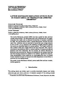
To solve Eqs. 共8兲 and 共9兲 we use a Lattice Boltzmann scheme on a lattice of size Lx ⫻ Ly in which each site is connected to nearest and next-to-nearest neighbors. This is one of the simplest geometries which reproduce correctly the Navier-Stokes equations in continuum limit and is shown in Fig. 1. Horizontal and vertical links have length ⌬x and diagonal links 冑2⌬x. On each site r nine lattice velocity vecx tors ei are defined. They have modulus 兩ei兩 = ⌬t⌬LB ⬅ c, being ⌬tLB the time step, for i = 1, 2, 3, 4, and modulus 兩ei兩 = 冑2c for

026701-2

PHYSICAL REVIEW E 80, 026701 共2009兲

HYBRID LATTICE BOLTZMANN MODEL FOR BINARY…

i = 5, 6, 7, 8. Moreover, the zero velocity vector e0 = 0 is defined. A set of distribution function 兵f i共r , t兲其 is defined on each lattice site r at each time t. In the LB scheme for simple fluids 关1兴 the distribution functions evolve during the time step ⌬tLB according to a single relaxation-time Boltzmann equation 关23兴 f i共r + ei⌬tLB,t + ⌬tLB兲 − f i共r,t兲 = −

⌬tLB 关f i共r,t兲 − f eq i 共r,t兲兴, ␶

cept for the formal substitution u → uⴱ, where uⴱ is given by 1 nuⴱ = 兺 f iei + F⌬tLB , 2 i

F being the force density acting on the fluid and uⴱ the physical velocity. The expression of F for our case will be given later. The forcing term Fi can be expressed as a power series at the second order in the lattice velocity 关25兴

冋

共11兲 where ␶ is a relaxation parameter and f eq i 共r , t兲 are the local equilibrium distribution functions. The total density n and the fluid momentum nu are defined by the following relations n = 兺 f i, i

nu = 兺 f iei ,

兺i

− f i兲ei = 0 ⇒ 兺

f eq i ei

冋

f eq i 共r,t兲 = ␻in 1 +

cs2

+

uu:共eiei − cs2I兲 2cs4

,

共15兲

where cs = c / 冑3 is the sound speed in this model, I is the unitary matrix and a suitable choice for the coefficients ␻i is ␻0 = 4 / 9, ␻i = 1 / 9 for i = 1 – 4, ␻i = 1 / 36 for i = 5 – 8. This form is such that

兺i f eqi ei␣ei␤ = ncs2␦␣␤ + nu␣u␤ .

f i共r + ei⌬tLB,t + ⌬tLB兲 − f i共r,t兲 =−

⌬tLB 关f i共r,t兲 − f eq i 共r,t兲兴 + ⌬tLBFi , ␶

共17兲

where Fi is the forcing term to be properly determined. The equilibrium distribution functions 共15兲 are not changed ex-

册

,

共19兲

共1兲 2 共2兲 f i = f 共0兲 i + ⑀fi + ⑀ fi + ¯ ,

共21兲

⳵ t = ⑀ ⳵ t1 + ⑀ 2⳵ t2 ,

共22兲

⳵ r = ⑀ ⳵ r1 ,

共23兲

F = ⑀ F 1,

A = ⑀ A 1,

B = ⑀ B 1,

C = ⑀C1 .

共24兲

We note that the force term is of first order in ⑀ 关26兴. The continuity and the Navier-Stokes equations are recovered in the following form:

⳵t共nu␤ⴱ 兲 + ⳵␣共nu␣ⴱ u␤ⴱ 兲 = − ⳵␤共ncs2兲 + F␤ + ⳵␣兵␩共⳵␣u␤ⴱ + ⳵␤u␣ⴱ 兲其 共25兲 in terms of the velocity uⴱ when the following expressions for the terms A, B, C: A = 0,

冉

B= 1−

冊

⌬tLB F, 2␶

冉

C= 1−

冊

⌬tLB 共uⴱF + Fuⴱ兲 2␶ 共26兲

共16兲

In order to simulate Eq. 共9兲 where a nonideal pressure tensor P␣␤ appears, we adopt a LB model with a forcing term following a derivation similar to that of Ref. 关12兴. In the case of Ref. 关12兴 the model was used to study forced simple fluids while we address the case of a binary mixture with interaction and interface contributions. The evolution equation of the distribution functions becomes

2cs4

and have to be consistent with the hydrodynamic equations. The continuum limit is obtained by using a ChapmanEnskog expansion in the Knudsen number ⑀,

共14兲

册

C:共eiei − cs2I兲

共20兲

f eq i ’s

ei · u

+

1

i

need to have some symmetries so that the Moreover, the Navier-Stokes equations are reproduced in the continuum limit. A convenient choice for the local equilibrium distribution functions of an ideal fluid in the case of a D2Q9 model is given by a second-order expansion in the fluid velocity u of the Mawwell-Boltzmann distribution 关24兴

cs2

兺i Fi = A, 兺i Fiei = B, 兺i Fieiei = cs2AI + 2 关C + CT兴,

共13兲

= nu.

B · ei

where A, B, and C are functions of F. The moments of the force verify the following relations

i

兺i 共f eqi − f i兲 = 0 ⇒ 兺i f eqi = n, 共f eq i

Fi = ␻i A +

共12兲

where u is the fluid velocity. The form of f eq i must be chosen so that the mass and momentum are locally conserved in each collision step, therefore the following relations must be satisfied:

共18兲

are used. The continuum Eqs. 共8兲 and 共25兲 can be also obtained by a Taylor expansion method. We remark that no spurious terms are present in the continuum equations except for a term of order uⴱ3 which is neglected in Eq. 共25兲. Such approximation is correct as far as uⴱ2 Ⰶ cs2 when the expansion 共15兲 is valid 关1兴. In the present formulation the second moment of the equilibrium distribution function 共16兲 does not need to be modified to include the effects of the pressure tensor as in previous models based on a free energy 关7兴. It is straightforward to show that the momentum defined in Eq. 共18兲 corresponds to an average between the pre- and postcollisional values of the velocity u which is the correct way to calculate it when a forcing term is introduced 关6,26兴. It is this value that appears in the continuum equations and is measured in simulations. As in the case of standard LBM 关1兴, the

026701-3

PHYSICAL REVIEW E 80, 026701 共2009兲

TIRIBOCCHI et al.

present model is characterized by the fact that ␨ = d2 ␩ with shear viscosity

␩ = ncs2⌬tLB

冉

冊

1 ␶ − . ⌬tLB 2

共27兲

In order to recover Eq. 共9兲 we have to require that F = ⵜ共ncs2 − pi兲 − ␸ ⵜ ␮ = − ␸ ⵜ ␮ .

共28兲 ncs2

correThe last equality comes from the fact the term sponds in LBM to the ideal gas pressure pi 关1兴. Finally, the forcing term in Eq. 共17兲 has the form

冉

Fi = 1 −

冊冋

time steps is ⌬tLB = m⌬tFD, being m an integer. We denote any discretized function at time tn on a node 共xi , y j兲 共i = 1 , 2 , . . . , Lx ; j = 1 , 2 , . . . , Ly兲 of the lattice by g共xi , y j , tn兲 = gnij. At each time step we update ␸n → ␸n+1 using Eq. 共10兲 in two successive partial steps 关29兴. This allows to have a better numerical stability. In the first step we implement the convective term using an explicit Euler algorithm 关30兴

册

ei − uⴱ ei · uⴱ ⌬tLB ␻i + 4 ei · F 2␶ cs2 cs

共29兲

with uⴱ given by Eq. 共18兲.

␸n+1/2 = ␸n − ⌬tFD共␸n⳵␣u␣ⴱn + u␣ⴱn⳵␣␸n兲

where the velocity uⴱ comes from the solution of the LB equation. Note that the term ⳵␣u␣ⴱn has not been neglected since the fluid is not exactly incompressible. Indeed, the Navier-Stokes Eq. 共25兲 coming from the LBM contains some compressibility terms which can be anyway kept very small requiring that uⴱ2 Ⰶ cs2 关1兴. The derivatives in Eq. 共32兲 are discretized as follows:

⳵Dxuⴱx 兩nij =

B. Numerical calculation of the forcing term

The derivatives of the order parameter in the forcing term 共28兲 are calculated using a finite-difference scheme. In particular, we have adopted a stencil representation of finitedifference operators in the more general way to ensure higher isotropy 关16兴, which is known to reduce spurious velocities 关27,28兴. The schemes for the x derivative and the Laplacian operators are, respectively,

⳵Dx =

冤

冥

−M 0 M 1 −N 0 N , ⌬x −M 0 M

冤

R

共30兲

冥

Q R 1 2 ⵜD = 2 Q − 4共Q + R兲 Q , ⌬x R Q R

共32兲

⳵Dx␸兩nij

=

⳵Dx␸兩nij =

ⴱn ⴱn ux,共i+1兲j − ux,共i−1兲j

n ␸nij − ␸共i−1兲j

⌬x n ␸共i+1兲j − ␸nij

⌬x

,

共33兲

if

uⴱn x,ij ⬎ 0,

共34兲

if

uⴱn x,ij ⬍ 0,

共35兲

2⌬x

and analogously for the y components. The diffusive part of Eq. 共10兲 is implemented in the second update step using an explicit Euler algorithm as

␸n+1 = ␸n+1/2 + ⌬tFD⌫关aⵜ2␸n+1/2 + bⵜ2 f n − ␬ⵜ2共ⵜ2␸n+1/2兲兴, 共31兲

共36兲 where f = 共␸ 兲 and the operator ⵜ is discretized using the form given in Eq. 共31兲 with the standard choice Q = 1 and R = 0. Other choices using a more general stencil for discretizing ⵜ2 are possible though we checked that they did not provide any relevant difference. n

with 2N + 4M = 1 and Q + 2R = 1 to guarantee consistency between the continuous and discrete derivatives 关16兴. The subscript D in the symbols of derivatives denotes the discrete operator. In these schemes the central entry is referred to the lattice point where the derivative is computed, and the other entries are referred to the eight neighbor lattice sites. The discrete derivatives of the order parameter ␸ are computed by summing the values in the site and in the eight neighbors with the weights in the matrices 共30兲 and 共31兲. The y derivative is computed by transposing the matrix 共30兲. The choice of the free parameters N and Q is made in such a way that the spurious velocities are minimized 共see next section兲. We will refer to this case as the optimal choice 共OC兲. The values N = 1 / 2, M = 0, Q = 1, and R = 0 correspond to the standard central difference scheme denoted as SC. We will compare SC and OC in the following. C. Scheme for the convection-diffusion equation

The convection-diffusion Eq. 共10兲 is solved by using a finite-difference scheme. The function ␸共r , t兲 is defined on the nodes of the same lattice used for the LB scheme. The time is discretized in time steps ⌬tFD with time values tn = n⌬tFD, n = 1 , 2 , 3 , . . .. The relationship connecting the two

n 3

2

III. RESULTS AND DISCUSSION

We considered several test cases in order to validate our model. We used the values ⌬x = ⌬tLB = ⌬tFD = 1. In the free energy we adopted the parameters −a = b = 10−3, ␬ = −3a corresponding to an equilibrium interface of width ␰ ⯝ 5⌬x. The mobility ⌫ was set to 5 and the relaxation time ␶ / ⌬tLB was 1 unless differently stated. We first examined the relaxation to equilibrium of a planar sharp interface on a lattice of size Lx = Ly = 64 varying ␶ in the SC case. In all the cases the system correctly relaxes to the expected profile 共2兲. One example is reported in Fig. 2. In the case of a planar interface the fluid velocities uⴱ decay to negligible values as it should be at equilibrium when ⌬␮ = 0 and ⳵␣ P␣␤ = 0. We then studied a circular drop as a test for a case with interfaces not aligned with the lattice links. A drop with sharp interface of diameter 64⌬x was placed at the center of a lattice of size Lx = Ly = 128 and let equilibrate in the SC

026701-4

PHYSICAL REVIEW E 80, 026701 共2009兲

HYBRID LATTICE BOLTZMANN MODEL FOR BINARY…

TABLE I. Optimal values of N and Q for different values of ␶ and the corresponding values of the maximum spurious velocity 兩uⴱmax兩.

1

ϕ/ϕeq

0.5

0

-0.5

-1 10

15

20

25

30

35

40

45

N

Q

兩uⴱmax兩 / cs

0.6 0.8 1 1.2 5 10

0.3 0.3 0.3 0.3 0.3 0.3

3 2.5 2.5 2.5 2.5 2

0.0001753 0.0000603 0.0000365 0.0000267 0.0000088 0.0000062

50

x/∆x FIG. 2. Equilibrium profile of a planar interface on a lattice of size Lx = Ly = 64 in the SC case. The continuous line is the analytical result 共2兲 and data points are the results of simulations.

case. Interfaces relax to the expected profile without deforming the drop but spurious velocities appear as it can be seen in the upper panel of Fig. 3 in the case with ␶ / ⌬tLB = 5. We then used the OC scheme to verify whether spurious velocities could be reduced by using a more isotropic structure for the discrete spatial derivatives in the forcing term 共28兲. We scanned several values of N and Q in order to reduce the ⴱ 兩 on the whole lattice. maximum value of the velocity 兩umax The optimal values are summarized in the Table I. It is interesting to note that there is a couple of values N = 0.3 and Q = 2.5 which occurs more frequently. We verified that this choice is also effective in reducing spurious velocities even for the other values of ␶. For this choice of N and Q the maximum velocities differ only by a small percentage from the tabled values. Velocities can be greatly reduced with respect to the SC case as it can be visually observed in the lower panel of Fig. 3. We also tried to get an analytical estimate of the optimal values of N and Q in the following way. At equilibrium it holds that ⳵␣ P␣␤ = ␸⳵␤␮ = 共a␸ + 3b␸3兲⳵␤␸ − k␸⳵␤共ⵜ2␸兲 = 0. This expression depends on the first- and third-order deriva-

(a)

␶ / ⌬tLB

(b)

FIG. 3. Velocity patterns 共the same scale is used in both the panels兲 at equilibrium when ␶ / ⌬tLB = 5 in the SC case 共upper panel兲 and in the OC case 共lower panel兲. Empty spaces are due to negligible values of velocity. In both the cases the system has size Lx = Ly = 128.

tives. By using the stencils 共30兲 and 共31兲 we get for the discretized operators the expressions 1 1 − 2N 共⌬x兲2⳵x⳵2y + ¯ ⳵Dx = ⳵x + 共⌬x兲2⳵3x + 6 2

共37兲

and 2 = ⵜ2 + ⵜD

1 1−Q 共⌬x兲2⳵2x ⳵3y + ¯ , 共⌬x兲2共⳵4x + ⳵4y 兲 + 12 2 共38兲

so that

冋

1 1 1 − 2N 1 − Q + + ⳵Dx共ⵜD2 兲 = ⳵x共ⵜ2兲 + 共⌬x兲2⳵5x + 4 6 2 2 ⫻共⌬x兲2⳵3x ⳵2y +

冋

册

册

1 1 − 2N + 共⌬x兲2⳵x⳵4y + ¯ . 12 2 共39兲

By imposing that the error terms in the third-order derivative depending on N and Q vanish, we get N = 7 / 12⯝ 0.6 and Q = 7 / 6 ⯝ 1.2. However, this estimate does not correspond to the optimal results of Table I. This is due to the fact that these optimal values were found by considering the full dynamical problem with the whole set of equations where we minimized the spurious velocities. In the estimate after Eq. 共40兲 the coupling with the velocity field was not taken into account so that there is no a priori reason to expect the same optimal values for N and Q. A comparison of the spurious velocities in the SC and OC cases is shown in Fig. 4. By using the optimal choice OC the spurious velocities can be reduced by a factor approximately 10 with respect to the standard case SC over the whole range of ␶ values. The stencil forms 共30兲 and 共31兲 were also applied to the model of Ref. 关7兴 for nonideal fluids finding a comparable reduction in the magnitude of spurious velocities with respect to the standard case 关16兴. We then studied the motion of an equilibrated drop of diameter 64⌬x in a lattice of size Lx = 256, Ly = 128 under the effect of an external constant force that acts up to the time t / ⌬tLB = 500 and is then switched off. The additional force G = n共gx , 0兲⌬x2 / ⌬tLB acts on the total density. gx is in the range 关10−5 , 5 ⫻ 10−5兴 and the OC scheme is used. The overall system is set in motion rightward with increasing velocity

026701-5

PHYSICAL REVIEW E 80, 026701 共2009兲

TIRIBOCCHI et al.

t/∆tLB = 500

t/∆tLB = 3000

FIG. 4. Maximum spurious velocities as a function of ␶ in the SC case 共+兲 and in the OC case 共 䊊 兲.

until the force G is on, then it moves with constant speed. The choice of gx is such that the final velocity is much smaller than the speed of sound cs. The aim was to check whether the system is Galilean invariant and the drop is correctly convected by the flow. We monitored the shape of the drop and measured its center-of-mass velocity vCM . This is defined as the average velocity of the center of mass whose position is rCM 共t兲 =

兺ij␸ijrij共t兲 , 兺ij␸ij

(a)

共40兲

where the sum is over the lattice nodes rij inside the drop. This velocity represents the convection velocity and is compared with the fluid velocity v f 共t兲 = uⴱ关rCM 共t兲兴 at the center of mass given directly by the LBM. In Fig. 5 the comparison between the velocities vCM and v f along the x direction is shown in the case with gx = 3 ⫻ 10−5. It is evident that the two coincide indicating that the drop is correctly advected by the fluid. Moreover, its shape is not altered by motion as it can be seen in Fig. 6 where some configurations of the system at vCM x / cs , vf x / cs

t/∆tLB = 6000

0.02

(b) FIG. 6. Configurations of the advected drop at consecutive times. The system has size Lx = 256, Ly = 128. In the lower panel the drop, extracted from the system, is shown on an underlying mesh to better appreciate its shape.

different times are presented. Moreover, the drop is shown to make clear that it does not change in shape with time. We measured the ratio of the horizontal and vertical diameters finding that it stays almost constant with a deviation less than 3% from the value 1. If the advection velocity is higher, the drop will be slightly deformed being stretched along the x direction. This effect becomes negligible when increasing the surface tension 共4兲 via the parameter ␬.

0.015

0.01

0.005

IV. CONCLUSIONS 0

0

2000

4000

6000

8000

t / ∆tLB FIG. 5. Velocities of the center of mass of the drop vCMx 共 䊊 兲 and of the fluid v fx 共—兲 at the center of mass along the x direction as a function of time. The external force acts until the time t / ⌬tLB = 500.

In this paper we have considered a lattice Boltzmann method for binary mixtures with thermodynamics fixed by a free-energy functional. We used a mixed method, with continuity and Navier-Stokes equations simulated by LBM, and convection-diffusion equation by finite-difference schemes. Differently than in previous free-energy LBM formulations 关7兴, the interaction part in the pressure tensor is not intro-

026701-6

PHYSICAL REVIEW E 80, 026701 共2009兲

HYBRID LATTICE BOLTZMANN MODEL FOR BINARY…

duced by fixing the second moment of the LBM populations but by introducing a forcing term in the lattice equation. This approach is suggested by a microscopic picture and allows to obtain a continuum limit without spurious terms. On the other hand, the mixed or hybrid approach allows a reduction in the required memory and this can be relevant in performing large-scale simulations. In order to reduce spurious velocities, differential operators have been discretized by generalizing the usual lattice representations. Free parameters appear and their optimal values have been fixed by requiring that the maximum value of spurious velocities at equilibrium is minimized. We considered simple test situations, flat interfaces and single drops showing that the correct equilibrium profiles are reproduced. We found that spurious velocities are reduced of about an order of magnitude when a more general stencil is

applied to the derivatives in the forcing term of the LBM equations. We did not found any relevant difference by applying this procedure to the differential operators appearing in the convection-diffusion equation. We also checked that our method is stable in phase-separation studies, even if we have not reported the results of these simulations in this work. Finally, we checked the effective Galilean invariance of the system by advecting for some time interval by a constant force a configuration with one drop and then letting the system to evolve without forcing. For the cases considered, we did not observe relevant drop deformations, the drop being correctly advected by the surrounding fluid. In conclusion, we hope that this development of the free-energy LBM can be useful in future simulations of binary mixtures and complex fluids.

关1兴 R. Benzi, S. Succi, and M. Vergassola, Phys. Rep. 222, 145 共1992兲; S. Chen and G. D. Doolen, Annu. Rev. Fluid Mech. 30, 329 共1998兲; S. Succi, The Lattice Boltzmann Equation for Fluid Dynamics and Beyond 共Clarendon Press, Oxford, 2001兲. 关2兴 B. Dünweg and A. J. C. Ladd, Adv. Polym. Sci. 221, 89 共2009兲. 关3兴 V. M. Kendon, J.-C. Desplat, P. Bladon, and M. E. Cates, Phys. Rev. Lett. 83, 576 共1999兲. 关4兴 C. Denniston, E. Orlandini, and J. M. Yeomans, Phys. Rev. E 63, 056702 共2001兲. 关5兴 J. M. Yeomans, Annu. Rev. Comput. Phys. VII, 61 共1999兲. 关6兴 X. Shan and H. Chen, Phys. Rev. E 49, 2941 共1994兲. 关7兴 E. Orlandini, M. R. Swift, and J. M. Yeomans, Europhys. Lett. 32, 463 共1995兲; M. R. Swift, E. Orlandini, W. R. Osborn, and J. M. Yeomans, Phys. Rev. E 54, 5041 共1996兲. 关8兴 G. Gonnella, E. Orlandini, and J. M. Yeomans, Phys. Rev. Lett. 78, 1695 共1997兲. 关9兴 A. Lamura, G. Gonnella, and J. M. Yeomans, Europhys. Lett. 45, 314 共1999兲. 关10兴 M. E. Cates, S. M. Fielding, D. Marenduzzo, E. Orlandini, and J. M. Yeomans, Phys. Rev. Lett. 101, 068102 共2008兲. 关11兴 Q. Li and A. J. Wagner, Phys. Rev. E 76, 036701 共2007兲. 关12兴 Z. Guo, C. Zheng, and B. Shi, Phys. Rev. E 65, 046308 共2002兲. 关13兴 A. G. Xu, G. Gonnella, and A. Lamura, Physica A 362, 42 共2006兲. 关14兴 D. Marenduzzo, E. Orlandini, M. E. Cates, and J. M. Yeomans,

Phys. Rev. E 76, 031921 共2007兲. 关15兴 P. Lallemand and L. S. Luo, Int. J. Mod. Phys. B 17, 41 共2003兲; F. Dubois and P. Lallemand, e-print arXiv:0811.0599. 关16兴 C. M. Pooley and K. Furtado, Phys. Rev. E 77, 046702 共2008兲. 关17兴 A. J. Bray, Adv. Phys. 43, 357 共1994兲. 关18兴 J. S. Rowlinson and B. Widom, Molecular Theory of Capillarity 共Clarendon Press, Oxford, 1982兲. 关19兴 A. J. M. Yang, P. D. Fleming, and J. H. Gibbs, J. Chem. Phys. 64, 3732 共1976兲. 关20兴 R. Evans, Adv. Phys. 28, 143 共1979兲. 关21兴 S. R. De Groot and P. Mazur, Non-equilibrium Thermodynamics 共Dover Publications, New York, 1984兲. 关22兴 I. Rasin, S. Succi, and W. Miller, J. Comput. Phys. 206, 453 共2005兲. 关23兴 P. L. Bhatnagar, E. P. Gross, and M. Krook, Phys. Rev. 94, 511 共1954兲. 关24兴 Y. Qian, D. d’Humieres, and P. Lallemand, Europhys. Lett. 17, 479 共1992兲. 关25兴 A. J. C. Ladd and R. Verberg, J. Stat. Phys. 104, 1191 共2001兲. 关26兴 J. M. Buick and C. A. Greated, Phys. Rev. E 61, 5307 共2000兲. 关27兴 X. Shan, Phys. Rev. E 73, 047701 共2006兲. 关28兴 M. Sbragaglia, R. Benzi, L. Biferale, S. Succi, K. Sugiyama, and F. Toschi, Phys. Rev. E 75, 026702 共2007兲. 关29兴 S. M. Fielding, Phys. Rev. E 77, 021504 共2008兲. 关30兴 J. C. Strikwerda, Finite Difference Schemes and Partial Differential Equations 共Chapman and Hall, New York, 1989兲.

026701-7