Gabungan algoritma genetik dan pembelajaran mesin melampau digu- ...... where Q is a M Ã M permutation matrix that uses elementary vectors (vector, all of ..... fuzzy sets/rules so one benefit of T2FLC is a lower trade-off between modeling ...
STATUS OF THESIS HYBRID LEARNING ALGORITHMS FOR INTERVAL TYPETitle of thesis
2 FUZZY LOGIC SYSTEM TO MODEL NONLINEAR DYNAMIC SYSTEMS
I
SAIMA HASSAN
hereby allow my thesis to be placed at the Information Resource Center (IRC) of Universiti Teknologi PETRONAS (UTP) with the following conditions: 1. The thesis becomes the property of UTP 2. The IRC of UTP may make copies of the thesis for academic purposes only. 3. This thesis is classified as Confidential Non-confidential If this thesis is confidential, please state the reason:
The contents of the thesis will remain confidential for
years.
Remarks on disclosure:
Endorsed by:
Signature of Author
Signature of Supervisor
Permanent Address: Ghazi Amanat Shah Baba Road, Afghan Colony, 26000 Peshawar, KPK, Pakistan
Name of Supervisor: Assoc. Prof. Dr. Jafreezal Jaafar
Date:
Date:
UNIVERSITI TEKNOLOGI PETRONAS HYBRID LEARNING ALGORITHMS FOR INTERVAL TYPE-2 FUZZY LOGIC SYSTEM TO MODEL NONLINEAR DYNAMIC SYSTEMS
by
SAIMA HASSAN
The undersigned certify that they have read, and recommend to the Postgraduate Studies Programme for acceptance of this thesis for the fulfilment of the requirements for the degree stated.
Signature: Main Supervisor:
Assoc. Prof. Dr. Jafreezal Jaafar
Signature: Co-Supervisor:
Dr. Abbas Khosravi
Signature: Head of Department: Assoc. Prof. Dr. Wan Fatimah binti Wan Ahmad Date:
HYBRID LEARNING ALGORITHMS FOR INTERVAL TYPE-2 FUZZY LOGIC SYSTEM TO MODEL NONLINEAR DYNAMIC SYSTEMS
by
SAIMA HASSAN
A Thesis Submitted to the Postgraduate Studies Programme as a Requirement for the Degree of
DOCTOR OF PHILOSOPHY INFORMATION TECHNOLOGY UNIVERSITI TEKNOLOGI PETRONAS BANDAR SERI ISKANDAR PERAK
August 2016
DECLARATION OF THESIS HYBRID LEARNING ALGORITHMS FOR INTERVAL TYPETitle of thesis
2 FUZZY LOGIC SYSTEM TO MODEL NONLINEAR DYNAMIC SYSTEMS
I
SAIMA HASSAN
hereby declare that the thesis is based on my original work except for quotations and citations which have been duly acknowledged. I also declare that it has not been previously or concurrently submitted for any other degree at UTP or other institutions.
Witnessed by
Signature of Author
Signature of Supervisor
Permanent Address: Ghazi Amanat Shah Baba Road, Afghan Colony, 26000 Peshawar, KPK, Pakistan
Name of Supervisor: Assoc. Prof. Dr. Jafreezal Jaafar
Date:
Date:
iv
DEDICATION
To my beloved parents, who trust in me more than anybody and made me realize that I am worth everything in this world.
v
ACKNOWLEDGEMENTS
In the name of Allah, the Most Gracious and the Most Merciful. All praises to Allah, and peace and blessings be upon to His messenger, Muhammad (S.A.W). I owe my gratitude to all those people with the help, support and inspiration of whom the completion of this thesis becomes possible. First of all, I would like to thank my first supervisor AP. Dr. Jafreezal Jaafar for giving me the freedom to explore on my own. I appreciate his trust and consistent support throughout my research. I would like to thank my second supervisor Dr. Abbas Khosravi from Deakin University Australia, providing me with useful insights into the topic with his guidance. He always responded to my questions and queries promptly. I would also like to express very special thanks to Dr Mojtaba Ahmadieh Khanesar for his extended help in my research. I am grateful for his technical discussion, suggestions and timely review of my thesis. I wish to thank all the examiners for their constructive comments during each symposium presentation. I wish to express my sincere thanks to all the staff of the Department of Computer and Information Sciences, Universiti Technologi PETRONAS (UTP). I would like to acknowledge the UTP graduate assistance ship scheme for financial support in and to the Kohat University of Science and Technology, KPK, Pakistan for providing opportunity for this study at UTP. I am indebted to my parents and to my dearest sibling for their love, dream and support throughout my life. I am thankful to my parents-in-law for their support and prayers. I would like to show my gratitude to my husband, Tariq, without who this effort would have been worth nothing. I wish to thank my wonderful children, Salaar, Ummamah and our new addition Jumanah; they are the love and pride of my life.
vi
ABSTRACT
Interval type-2 fuzzy logic system (IT2FLS) have extensively been applied to various engineering problems, e.g. identification, prediction, control, pattern recognition, etc. In the design of IT2FLS its antecedent and consequent parameters need to be chosen on expert’s knowledge. IT2FLS needs more parameters than its type-1 counterpart due to the presence of foot-print-of-uncertainty. The higher number of parameters make the design procedure of IT2FLS a challenging task. Since the consequent part parameters appear linearly in the output of IT2FLS, the derivative based methods can be easily implemented to optimize these parameters. Whereas, the antecedent part parameters appear nonlinearly in the output and random optimization techniques are preferred to be used for their optimization. A combination of genetic algorithm and extreme learning machine is utilized here to optimize the parameters of the IT2FLS. Genetic algorithm is utilized to search the optimal antecedent parameters, whereas the extreme learning machine is employed to analytically tune the consequent parameters. Once the effective forecasting performance is achieved from the hybrid of genetic algorithm and extreme learning machine, it is decided to apply more sophisticated algorithm to obtain the optimal parameters for the IT2FLS. Therefore, another hybrid algorithm based on artificial bee colony optimization algorithm and the extreme learning machine is proposed to optimize the parameters of the IT2FLS. The proposed designs of IT2FLS are applied to model two simulated and two real world bench-mark problems. Comparative forecasting analysis of three approaches for the generation of antecedent part on the Mackey-Glass time series data revealed the importance of optimal parameters for the extreme learning machine-based-IT2FLS. Comparison of the proposed algorithms with the existing hybrid learning algorithms of IT2FLS have proved these as new alternatives of hybrid learning algorithms of IT2FLS for modeling real-world problems. vii
ABSTRAK
Sistem Interval fuzzy logic type-2 (IT2FLS) digunakan dengan meluas dalm masalah kejuruteraan seperti identifikasi, ramalan, kawalan, pengecaman corak, dan lain-lain. Dalam rekabentuk IT2FLS, parameter antecedent dan consequent perlu dipilih berdasarkan pengetahuan pakar. IT2FLS memerlukan lebih banyak parameter berbanding Fuzzy Logic type-1 kerana kehadiran ketidakpastian atau kekaburan (foot-print-of-uncertainty). Pertambahan jumlah parameter menjadikan prosedur rekabentuk IT2FLS satu tugas yang mencabar. Kemunculan sebahagian daripada consequent parameter secara linear dalam output IT2FLS, membolehkan kaedah derivative dilaksanakan dengan mudah untuk mengoptimumkan parameter ini. Manakala, antecedent parameter yang sebahagian outputnya dipaparkan secara nonlinear dan teknik pengoptimuman secara rawak telah digunakan. Gabungan algoritma genetik dan pembelajaran mesin melampau digunakan untuk mengoptimumkan parameter IT2FLS. Algoritma genetik digunakan untuk mencari parameter yang optimum, manakala mesin pembelajaran melampau digunakan untuk melaras consequent parameter secara analitikal. Setelah prestasi peramalan yang berkesan dicapai secara hibrid, algoritma yang lebih komplex digunakan untuk mendapatkan parameter yang lebih optimum. Oleh itu, satu lagi algoritma hibrid yang berasaskan algoritma pengoptimuman koloni lebah dan mesin pembelajaran yang melampau telah digunakan. Rekabentuk yang dicadangkan IT2FLS untuk dua model simulasi dan dua masalah sebenar sebagai penanda aras. Analisis ramalan dijalankan untuk perbandingan tiga pendekatan bagi penjanaan bahagian antecedent keatas data siri masa (time series data) Mackey-Glass. Ia mendedahkan bahawa kepentingan parameter optimum untuk pembelajaran mesin melampau bagi IT2FLS. Perbandingan algoritma yang dicadangkan dengan algoritma pembelajaran hibrid sediaada, IT2FLS telah membuktikan bahawa algoritma pembelajaran hibrid IT2FLS merupakan model alternatif untuk viii
penyelesaian masalah dunia sebenar.
ix
In compliance with the terms of the Copyright Act 1987 and the IP Policy of the university, the copyright of this thesis has been reassigned by the author to the legal entity of the university, Institute of Technology PETRONAS Sdn Bhd. Due acknowledgment shall always be made of the use of any material contained in, or derived from, this thesis. c
Saima Hassan, 2016 Institute of Technology PETRONAS Sdn Bhd All rights reserved.
x
TABLE OF CONTENT ABSTRACT............................................................................................................................. vii ABSTRAK .............................................................................................................................. viii TABLE OF CONTENT ............................................................................................................ xi LIST OF TABLES .................................................................................................................. xvi LIST OF FIGURES .............................................................................................................. xviii LIST OF ABREVIATIONS ................................................................................................. xxiii NOMENCLATURE .............................................................................................................. xxv
CHAPTER 1 INTRODUCTION ................................................................................... 1 1.1 Research Background ........................................................................................ 1 1.2 Motivation.......................................................................................................... 3 1.3 Problem Statement ............................................................................................. 6 1.4 Research Questions ............................................................................................ 6 1.5 Research Objectives........................................................................................... 7 1.6 Proposed Hypothesis ......................................................................................... 8 1.7 Scope of the Thesis ............................................................................................ 8 1.7.1 Interval Type-2 Fuzzy Logic System .................................................... 9 1.7.2 Genetic and Artificial Bee Colony Algorithms ................................... 10 1.7.3 Extreme Learning Machine ................................................................. 10 1.7.4 Hybrid Model ...................................................................................... 10 1.8 Significance of the Research ........................................................................... 10 1.9 Organization of the Thesis ............................................................................... 11 1.10 Summary of the Chapter ................................................................................ 12 CHAPTER 2 LITERATURE REVIEW ...................................................................... 14 2.1 Introduction...................................................................................................... 14 2.2 Type-1 Fuzzy Sets and System ........................................................................ 16 2.2.1 Type-1 Fuzzy Sets (T1FSs) ................................................................. 16 2.2.2 Type-1 Fuzzy Sets Operations ............................................................ 20 2.2.3 Type-1 Fuzzy Logic System (T1FLS) ................................................ 21 2.2.3.1 Fuzzifier ................................................................................... 21 xi
2.3
2.4
2.5
2.2.3.2
Rule base . . . . . . . . . . . . . . . . . . . . . . . .
22
2.2.3.3
Inference . . . . . . . . . . . . . . . . . . . . . . . .
22
2.2.3.4
Defuzzification . . . . . . . . . . . . . . . . . . . . .
23
Type-2 Fuzzy Sets and Systems . . . . . . . . . . . . . . . . . . . . . .
23
2.3.1
Uncertainty and Fuzzy Sets . . . . . . . . . . . . . . . . . . . .
23
2.3.2
Type-2 Fuzzy Sets (T2FSs) . . . . . . . . . . . . . . . . . . . .
25
2.3.3
Interval Type-2 Fuzzy Sets (IT2FSs) . . . . . . . . . . . . . . .
27
2.3.4
Type-2 Fuzzy Sets Operations . . . . . . . . . . . . . . . . . .
28
2.3.5
Type-2 Fuzzy Logic Systems (T2FLS) . . . . . . . . . . . . . .
28
2.3.6
Interval Type-2 Fuzzy Logic System (IT2FLS) . . . . . . . . .
29
Takagi-Sugeno-Kang Fuzzy Logic System . . . . . . . . . . . . . . . .
29
2.4.1
Type-1 Takagi-Sugeno-Kang Fuzzy Logic System . . . . . . . .
30
2.4.2
Type-2 Takagi-Sugeno-Kang Fuzzy Logic System . . . . . . . .
30
2.4.3
Interval Type-2 Takagi-Sugeno-Kang Fuzzy Logic System . . .
31
Learning algorithms of Type-2 Fuzzy Logic System in Existing Literature 34 2.5.1
2.5.2
Derivative-Based or Gradient Descent-Based Learning Algorithms . . . . . . . . . . . . . . . . . . . . . . . . . . . . . . .
38
2.5.1.1
Back-Propagation Algorithms . . . . . . . . . . . . .
38
2.5.1.2
Levenberg-Marquardt Algorithm . . . . . . . . . . .
39
2.5.1.3
Kalman filter-based Algorithm . . . . . . . . . . . . .
40
2.5.1.4
Least Square Method . . . . . . . . . . . . . . . . . .
41
2.5.1.5
Radial Basis Function . . . . . . . . . . . . . . . . .
41
2.5.1.6
Simplex Method . . . . . . . . . . . . . . . . . . . .
42
2.5.1.7
Extreme Learning Machine . . . . . . . . . . . . . .
43
Derivative-free or Gradient free Learning Algorithms . . . . . .
43
2.5.2.1
Genetic Algorithm . . . . . . . . . . . . . . . . . . .
44
2.5.2.2
Particle Swarm Optimization . . . . . . . . . . . . .
46
2.5.2.3
Ant Colony Optimization . . . . . . . . . . . . . . .
47
2.5.2.4
Bee Colony Optimization . . . . . . . . . . . . . . .
49
2.5.2.5
Simulated Annealing . . . . . . . . . . . . . . . . . .
50
2.5.2.6
Sliding Mode Theory . . . . . . . . . . . . . . . . . .
50
xii
2.5.2.7
Others . . . . . . . . . . . . . . . . . . . . . . . . .
51
Hybrid Learning Algorithms . . . . . . . . . . . . . . . . . . .
52
2.5.3.1
Derivative-based Hybrid Learning Algorithms . . . .
53
2.5.3.2
Other Combinations of Hybrid Learning Algorithms .
54
Extreme Learning Machine (ELM) . . . . . . . . . . . . . . . . . . . .
56
2.6.1
Fuzzy-ELM . . . . . . . . . . . . . . . . . . . . . . . . . . . .
59
2.6.2
Optimal-ELM . . . . . . . . . . . . . . . . . . . . . . . . . . .
60
2.7
Artificial Bee Colony Optimization Algorithm . . . . . . . . . . . . . .
61
2.8
Critical Analysis on Learning Algorithms of IT2FLS . . . . . . . . . .
65
2.9
Summary . . . . . . . . . . . . . . . . . . . . . . . . . . . . . . . . .
70
CHAPTER 3 Methodology . . . . . . . . . . . . . . . . . . . . . . . . . . . .
73
2.5.3
2.6
3.1
Discussion and Rationale for Choice of Approach . . . . . . . . . . . .
74
3.2
Research Framework . . . . . . . . . . . . . . . . . . . . . . . . . . .
77
3.3
Optimization of Interval Type-2 Fuzzy Logic System using Extreme
3.4
Learning Machine (IT2FELM) . . . . . . . . . . . . . . . . . . . . . .
79
3.3.1
Identification of the antecedent parameters . . . . . . . . . . . .
79
3.3.2
Defining the consequents . . . . . . . . . . . . . . . . . . . . .
80
3.3.3
Tuning of the consequents . . . . . . . . . . . . . . . . . . . .
81
Hybrid Learning Algorithm of ELM and GA for the design of IT2FLS (GA-IT2FELM) . . . . . . . . . . . . . . . . . . . . . . . . . . . . . .
84
3.4.1
Chaos Determination in Data . . . . . . . . . . . . . . . . . . .
86
3.4.2
Data Preprocessing . . . . . . . . . . . . . . . . . . . . . . . .
86
3.4.2.1
Normalization and Data division . . . . . . . . . . . .
87
3.4.2.2
Selection of inputs . . . . . . . . . . . . . . . . . . .
87
3.4.3
Structure of the Interval Type-2 Fuzzy Logic System . . . . . .
87
3.4.4
Antecedent Parameters Learning using Genetic Algorithm . . .
88
3.4.5
Encoding Scheme of IT2FLS Using GA . . . . . . . . . . . . .
89
3.4.6
Objective Function . . . . . . . . . . . . . . . . . . . . . . . .
90
3.4.7
GA Operations . . . . . . . . . . . . . . . . . . . . . . . . . .
90
3.4.8
Computing the Performance Measures . . . . . . . . . . . . . .
91
xiii
3.5
3.6
Hybrid Learning Algorithm of ELM and ABC for the design of IT2FLS (ABC-IT2FELM) . . . . . . . . . . . . . . . . . . . . . . . . . . . . .
91
3.5.1
Structure of the Interval Type-2 Fuzzy Logic System . . . . . .
93
3.5.2
Antecedent Parameters Learning using ABC . . . . . . . . . . .
93
3.5.3
Encoding Scheme of IT2FLS Using ABC . . . . . . . . . . . .
93
3.5.4
Objective Function . . . . . . . . . . . . . . . . . . . . . . . .
94
3.5.5
Computing the Performance Measures . . . . . . . . . . . . . .
94
Model Verification . . . . . . . . . . . . . . . . . . . . . . . . . . . . .
95
3.6.1
Quantitative Forecasting Measures . . . . . . . . . . . . . . . .
96
3.6.1.1
Root Mean Square Error (RMSE) . . . . . . . . . . .
96
3.6.1.2
Mean Absolute Percentage Error(MAPE) . . . . . . .
97
3.6.1.3
Mean Absolute Scaled Error (MASE) . . . . . . . . .
97
3.6.1.4
Modified MAPE . . . . . . . . . . . . . . . . . . . .
97
3.6.1.5
Test Error J . . . . . . . . . . . . . . . . . . . . . . .
98
3.6.1.6
Regression Analysis R2 . . . . . . . . . . . . . . . .
98
Comparative Model for Evaluation . . . . . . . . . . . . . . . .
99
3.6.2.1
GA-Kalman filter based algorithm for IT2FLS . . . .
99
3.6.2.2
ABC-Kalman filter based algorithm for IT2FLS . . .
99
Summary of the Chapter . . . . . . . . . . . . . . . . . . . . . . . . .
99
3.6.2
3.7
CHAPTER 4 Empirical Analysis of the Proposed Models on Real World Dynamic Systems . . . . . . . . . . . . . . . . . . . . . . . . . . . . 101 4.1
Real-World Data for Model Analysis . . . . . . . . . . . . . . . . . . . 102 4.1.1
The Estimation of the low Voltage Electrical Line Length in Rural Towns (ELE-1) . . . . . . . . . . . . . . . . . . . . . . . . 102
4.1.2
The Estimation of the Medium Voltage Electrical Line Maintenance Cost (ELE-2) . . . . . . . . . . . . . . . . . . . . . . . . 103
4.2
4.3
Experimental Setup . . . . . . . . . . . . . . . . . . . . . . . . . . . . 103 4.2.1
Parameters Setting . . . . . . . . . . . . . . . . . . . . . . . . 104
4.2.2
Experimental Procedure . . . . . . . . . . . . . . . . . . . . . 105
Forecasting Analysis on the Estimation of the low Voltage Electrical Line Length in Rural Towns . . . . . . . . . . . . . . . . . . . . . . . 107 xiv
4.4
Forecasting Analysis on the Estimation of the Medium Voltage Electrical Line Maintenance Cost . . . . . . . . . . . . . . . . . . . . . . . . 116
4.5
4.6
Comparative Analysis . . . . . . . . . . . . . . . . . . . . . . . . . . . 125 4.5.1
Training Time Analysis . . . . . . . . . . . . . . . . . . . . . . 125
4.5.2
Improvement Analysis . . . . . . . . . . . . . . . . . . . . . . 127
4.5.3
Comparison With the Existing Literature . . . . . . . . . . . . . 129
Summary of the Chapter . . . . . . . . . . . . . . . . . . . . . . . . . 132
CHAPTER 5 Empirical Analysis of the Proposed Models on Simulated Data . . 133 5.1
5.2
Simulated Data for Model Analysis . . . . . . . . . . . . . . . . . . . . 133 5.1.1
Mackey-Glass Time Series Data . . . . . . . . . . . . . . . . . 134
5.1.2
Mackey-Glass Time Series With Added Noise . . . . . . . . . . 135
Experimental Setup . . . . . . . . . . . . . . . . . . . . . . . . . . . . 137 5.2.1
Parameters Setting . . . . . . . . . . . . . . . . . . . . . . . . 137
5.2.2
Experimental Procedure . . . . . . . . . . . . . . . . . . . . . 139 5.2.2.1
Manual Selection of the Antecedent Parameters of the IT2FELM . . . . . . . . . . . . . . . . . . . . . . . . 141
5.2.2.2
Randomly Generated Antecedent Parameters of the IT2FELM . . . . . . . . . . . . . . . . . . . . . . . . 142
5.2.2.3 5.3
Optimized Antecedent Parameters of the IT2FELM . . 143
Forecasting Analysis of the Proposed Design of IT2FLS . . . . . . . . . 143 5.3.1
Largest Lyapunove exponent (LLE) . . . . . . . . . . . . . . . 144
5.3.2
Forecasting Analysis on the Noise-free Mackey-Glass Time Series Data . . . . . . . . . . . . . . . . . . . . . . . . . . . . . . 145
5.3.3
Forecasting Analysis on the Mackey-Glass Time Series Data with Added Noise . . . . . . . . . . . . . . . . . . . . . . . . . 151
5.4
Forecasting Analysis of the IT2 fuzzy-ELM with optimal parameters . . 165 5.4.1
Forecasting Analysis on the Noise-free Mackey-Glass Time Series Data . . . . . . . . . . . . . . . . . . . . . . . . . . . . . . 166
5.4.2
Forecasting Analysis on the Noisy Mackey-Glass Time Series Data . . . . . . . . . . . . . . . . . . . . . . . . . . . . . . . . 172
5.5
Comparative Analysis . . . . . . . . . . . . . . . . . . . . . . . . . . . 179 xv
5.6
5.5.1
Training Time Analysis . . . . . . . . . . . . . . . . . . . . . . 179
5.5.2
Improvement Analysis . . . . . . . . . . . . . . . . . . . . . . 181
5.5.3
Comparison With the Existing Literature . . . . . . . . . . . . . 182
Summary of the Chapter . . . . . . . . . . . . . . . . . . . . . . . . . 187
CHAPTER 6 Conclusions and Future Directions . . . . . . . . . . . . . . . . . 189 6.1
Research Summary . . . . . . . . . . . . . . . . . . . . . . . . . . . . 189 6.1.1
Research Questions Revisited . . . . . . . . . . . . . . . . . . 191 6.1.1.1
Hybrid learning algorithms for the design of IT2FLS: 191
6.1.1.2
Optimal parameters of an IT2FELM . . . . . . . . . . 192
6.1.1.3
The impact of FOU size on the forecasting performance of IT2FLS . . . . . . . . . . . . . . . . . . . . 193
6.1.1.4 6.1.2
Forecasting ability of the proposed models . . . . . . 193
Discussion on Research Objectives . . . . . . . . . . . . . . . . 194
6.2
Research Contribution . . . . . . . . . . . . . . . . . . . . . . . . . . . 195
6.3
Limitations . . . . . . . . . . . . . . . . . . . . . . . . . . . . . . . . 197
6.4
Future Work . . . . . . . . . . . . . . . . . . . . . . . . . . . . . . . . 198
REFERENCES . . . . . . . . . . . . . . . . . . . . . . . . . . . . . . . . . . . 199
xvi
LIST OF TABLES
2.1
Summary of T2 TSK FLS. . . . . . . . . . . . . . . . . . . . . . . . .
2.2
Summary of the existing learning algorithms for type-2 fuzzy logic sys-
31
tem. . . . . . . . . . . . . . . . . . . . . . . . . . . . . . . . . . . . .
66
3.1
Elementary Vectors . . . . . . . . . . . . . . . . . . . . . . . . . . . .
83
4.1
Variables Used for the ELE-1 Problem. . . . . . . . . . . . . . . . . . . 102
4.2
Variables Used for the ELE-2. . . . . . . . . . . . . . . . . . . . . . . 103
4.3
Parameter Used for the ELE-1 Data . . . . . . . . . . . . . . . . . . . 110
4.4
Results Comparison of the Models on ELE-1 Data . . . . . . . . . . . . 114
4.5
Parameter Used for ELE-2 . . . . . . . . . . . . . . . . . . . . . . . . 118
4.6
Result Comparison of the Models on ELE-2 Data . . . . . . . . . . . . 123
4.7
MAPE% Improvement of the Proposed Hybrid Learning Algorithms for IT2FLS with the ELE-1 . . . . . . . . . . . . . . . . . . . . . . . . . . 128
4.8
MAPE% Improvement of the Proposed Hybrid Learning Algorithms for IT2FLS with ELE-2 . . . . . . . . . . . . . . . . . . . . . . . . . . . . 128
4.9
Result Comparison of the proposed model With Existing Literature for ELE-1 Data. . . . . . . . . . . . . . . . . . . . . . . . . . . . . . . . . 129
4.10 Result Comparison of the Proposed Models With Existing Literature for the ELE-2 Data. . . . . . . . . . . . . . . . . . . . . . . . . . . . . . . 131 5.1
Parameters of Mackey-Glass Time Series Data . . . . . . . . . . . . . . 135
5.2
Parameters used for Mackey-Glass Time Series Data . . . . . . . . . . 139
5.3
LLE of the noise free and noisy Mackey-Glass Time Series Data. . . . . 144
5.4
Forecast Comparison of the Proposed Models . . . . . . . . . . . . . . 150
5.5
Estimated Values of R2 of the Models for the Noisy Mackey-Glass Time Series Data . . . . . . . . . . . . . . . . . . . . . . . . . . . . . . . . 161
5.6
Selected Values of Sigma for the IT2 Fuzzy MFs. . . . . . . . . . . . . 166 xvii
5.7
The RMSE of IT2FELMs with Different FOUs and number of MFs . . 170
5.8
The Selected Values of Sigma for the MFs of the IT2FELM for the Noisy Mackey-Glass Time Series Data . . . . . . . . . . . . . . . . . . 173
5.9
RMSEs of IT2FELM With Different Sizes of FOUs For the Noisy MackeyGlass Time Series Data . . . . . . . . . . . . . . . . . . . . . . . . . . 174
5.10 MAPE% Improvement of the Proposed Hybrid Learning algorithms for the noise-free Mackey-Glass time series data. . . . . . . . . . . . . . . 181 5.11 MAPE% Improvement of the Proposed Hybrid Learning Algorithms with the Noisy Mackey-Glass Time Series Data . . . . . . . . . . . . . 183 5.12 RMSE Comparison of the Mackey-Glass Time Series Data With Existing Literature. . . . . . . . . . . . . . . . . . . . . . . . . . . . . . . . 184 5.13 RMSE Comparison of the noisy Mackey-Glass Time Series Data With Existing Literature. . . . . . . . . . . . . . . . . . . . . . . . . . . . . 186
xviii
LIST OF FIGURES
1.1
Scope of the thesis. . . . . . . . . . . . . . . . . . . . . . . . . . . . .
9
2.1
Classical Set with two values “0” & “1”. . . . . . . . . . . . . . . . . .
17
2.2
Gaussian type-1 fuzzy MFs [Mendel, 2001]. . . . . . . . . . . . . . . .
18
2.3
Type-1 fuzzy set with different MFs [Jang and Sun, 1997]. . . . . . . .
20
2.4
Type-1 fuzzy logic system block diagram [Mendel, 2001]. . . . . . . . .
22
2.5
Gaussian T2 fuzzy MF (FOU) [Mendel and John, 2002]. . . . . . . . .
26
2.6
Type-2 fuzzy set with different MFs. . . . . . . . . . . . . . . . . . . .
27
2.7
Block diagram of T2FLS [Karnik et al., 1999]. . . . . . . . . . . . . . .
29
2.8
(a) Annual number of publications for type-1 and type-2 fuzzy logic theory, (b) Annual number of conference and journal publications for type2 fuzzy logic theory. . . . . . . . . . . . . . . . . . . . . . . . . .
35
The annual number of publication on fuzzy learning. . . . . . . . . . .
35
2.10 Learning parts of a T2FLS. . . . . . . . . . . . . . . . . . . . . . . . .
37
2.11 Different learning methods for T2FLS. . . . . . . . . . . . . . . . . . .
38
2.12 Structure of ELM. . . . . . . . . . . . . . . . . . . . . . . . . . . . . .
57
2.9
3.1
Optimization of the fuzzy inference system with the interaction of evolutionary algorithms. . . . . . . . . . . . . . . . . . . . . . . . . . . .
3.2
74
Research framework for the design of IT2FLS using hybrid learning algorithms. . . . . . . . . . . . . . . . . . . . . . . . . . . . . . . . . .
78
3.3
Flowchart of IT2FELM. . . . . . . . . . . . . . . . . . . . . . . . . . .
79
3.4
Flowchart of the hybrid learning algorithm-1 (GA-IT2FELM). . . . . .
85
3.5
Encoding of IT2 fuzzy parameters into a population of chromosome. . .
89
3.6
Flowchart of the hybrid learning algorithm-2 of IT2FLS (ABC-IT2FELM). 92
3.7
Encoding of IT2 fuzzy parameters into a solution of food sources. . . .
4.1
3D view of a data sample of the ELE-1 data. . . . . . . . . . . . . . . . 104 xix
94
4.2
3D view of a data sample of the ELE-2 data. . . . . . . . . . . . . . . . 105
4.3
Experimental flow diagram. . . . . . . . . . . . . . . . . . . . . . . . . 106
4.4
Forecast of IT2FELM along actual data for ELE-1. . . . . . . . . . . . 108
4.5
Error histogram of IT2FELM for ELE-1. . . . . . . . . . . . . . . . . . 108
4.6
Scatter plot of IT2FELM for ELE-1. . . . . . . . . . . . . . . . . . . . 109
4.7
Generalization performance of the models on ELE-1. . . . . . . . . . . 111
4.8
Forecasted output of ELE-1 data continued... . . . . . . . . . . . . . . . 111
4.8
Forecasted output of ELE-1 data . . . . . . . . . . . . . . . . . . . . . 112
4.9
Error histograms of ELE-1 data. . . . . . . . . . . . . . . . . . . . . . 113
4.10 Scatter plots of the ELE-1 data. . . . . . . . . . . . . . . . . . . . . . . 115 4.11 Comparison of the forecasts of all models along actual data. . . . . . . . 116 4.12 Forecast of IT2FELM along actual data for ELE-2. . . . . . . . . . . . 117 4.13 Error histogram of IT2FELM for ELE-2. . . . . . . . . . . . . . . . . . 117 4.14 Scatter plot of IT2FELM for ELE-2. . . . . . . . . . . . . . . . . . . . 118 4.15 Generalization performance of the models on ELE-2. . . . . . . . . . . 119 4.16 Forecasted output of the models for ELE-2 continued... . . . . . . . . . 120 4.16 Forecasted output of the models for ELE-2. . . . . . . . . . . . . . . . 121 4.17 Error histogram of the models for ELE-2. . . . . . . . . . . . . . . . . 121 4.18 Scatter plots of model for ELE-2 data. . . . . . . . . . . . . . . . . . . 124 4.19 Comparison of the forecasts of all models along actual data for ELE-2. . 125 4.20 Time performance of the proposed GA-IT2FELM and ABC-IT2FELM models for the ELE-1. . . . . . . . . . . . . . . . . . . . . . . . . . . . 126 4.21 Time performance of the proposed GA-IT2FELM and ABC-IT2FELM models for the ELE-2. . . . . . . . . . . . . . . . . . . . . . . . . . . . 127 5.1
Mackey-Glass time series data. . . . . . . . . . . . . . . . . . . . . . . 134
5.2
Mackey-Glass time series data with added noise. (a) 0dB, (b) 4dB, (c) 10dB
. . . . . . . . . . . . . . . . . . . . . . . . . . . . . . . . . . . 136
5.3
Mackey-Glass time series data embedded for forecasting. . . . . . . . . 138
5.4
Noisy Mackey-Glass time series data embedded for forecasting. . . . . 138
5.5
Experimental flow diagram. . . . . . . . . . . . . . . . . . . . . . . . . 139
5.6
Experiments with three design approaches of the antecedent parameters. 140 xx
5.7
Comparative analysis flow. . . . . . . . . . . . . . . . . . . . . . . . . 141
5.8
Gaussian T2 fuzzy MF with a fixed mean and uncertain deviation. . . . 143
5.9
Autocorrelation plots of the data. (a) Mackey-Glass with noise free, (b) noisy Mackey-Glass. . . . . . . . . . . . . . . . . . . . . . . . . . . . 145
5.10 Generalization ability of all the four models on noise-free MackeyGlass time series data. . . . . . . . . . . . . . . . . . . . . . . . . . . . 146 5.11 Forecasted output of Mackey-Glass time series data continued.... . . . . 147 5.11 Forecasted output of Mackey-Glass time series data. . . . . . . . . . . . 148 5.12 Error histograms of Mackey-Glass time series data. . . . . . . . . . . . 149 5.13 Scatter plot of all models for Mackey-Glass time series data. . . . . . . 151 5.14 Forecasted output of the models with noisy Mackey-Glass time series data continued... . . . . . . . . . . . . . . . . . . . . . . . . . . . . . . 152 5.14 Forecasted output of the models with noisy Mackey-Glass time series data. . . . . . . . . . . . . . . . . . . . . . . . . . . . . . . . . . . . . 153 5.15 Error of the models for the noisy Mackey-Glass time series data continued... . . . . . . . . . . . . . . . . . . . . . . . . . . . . . . . . . . . . 153 5.15 Error of the models for the noisy Mackey-Glass time series data. . . . . 154 5.16 Error histogram of the models with noisy Mackey-Glass time series data (0dB). . . . . . . . . . . . . . . . . . . . . . . . . . . . . . . . . . . . 155 5.17 Error histogram of the models with noisy Mackey-Glass time series data (10dB) . . . . . . . . . . . . . . . . . . . . . . . . . . . . . . . . . . . 156 5.18 Error histogram of the models with noisy Mackey-Glass time series data (20dB). . . . . . . . . . . . . . . . . . . . . . . . . . . . . . . . . . . 157 5.19 RMSE Comparison of the Models for the Noisy Mackey-Glass Time Series Data. . . . . . . . . . . . . . . . . . . . . . . . . . . . . . . . . 158 5.20 MAPE Comparison of the Models for the Noisy Mackey-Glass Time Series Data. . . . . . . . . . . . . . . . . . . . . . . . . . . . . . . . . 159 5.21 MASE Comparison of the Models for the Noisy Mackey-Glass Time Series Data. . . . . . . . . . . . . . . . . . . . . . . . . . . . . . . . . 160 5.22 J Comparison of the Models for the Noisy Mackey-Glass Time Series Data. . . . . . . . . . . . . . . . . . . . . . . . . . . . . . . . . . . . . 160 xxi
5.23 Comparison of the value of J of models for noisy Mackey-Glass time series data. . . . . . . . . . . . . . . . . . . . . . . . . . . . . . . . . . 161 5.24 Scatter plots of the models for the noisy Mackey-Glass time series data (0dB). . . . . . . . . . . . . . . . . . . . . . . . . . . . . . . . . . . . 162 5.25 Scatter plots of the models for the noisy Mackey-Glass time series data (10dB). . . . . . . . . . . . . . . . . . . . . . . . . . . . . . . . . . . 163 5.26 Scatter plots of the models for the noisy Mackey-Glass time series data (20dB). . . . . . . . . . . . . . . . . . . . . . . . . . . . . . . . . . . 164 5.27 RMSE comparison of the IT2FELM with the proposed GA-IT2FELM and ABC-IT2FELM models. . . . . . . . . . . . . . . . . . . . . . . . 165 5.28 IT2 fuzzy MF with different size of FOUs. . . . . . . . . . . . . . . . . 167 5.29 Uncertainty of the IT2 fuzzy sets with 3 MFs. . . . . . . . . . . . . . . 168 5.30 IT2 fuzzy MF with different size of FOUs. . . . . . . . . . . . . . . . . 169 5.31 Uncertainty of the IT2 fuzzy sets with 5 MFs. . . . . . . . . . . . . . . 170 5.32 RMSE of different FOUs and number of MFs. . . . . . . . . . . . . . . 171 5.33 Forecasting comparison of all the three design approaches for the MackeyGlass time series data. . . . . . . . . . . . . . . . . . . . . . . . . . . . 172 5.34 Forecasted output of IT2FELM with noisy Mackey-Glass time series data.175 5.35 Error histograms of the IT2FELM for the noisy Mackey-Glass time series data . . . . . . . . . . . . . . . . . . . . . . . . . . . . . . . . . . 176 5.36 Scatter plots of IT2FELM with random generated parameters for the noisy Mackey-Glass time series data. . . . . . . . . . . . . . . . . . . . 177 5.37 RMSE comparison of the different FOUs with the IT2FELM. . . . . . . 179 5.38 Time performance of the proposed models for Mackey-Glass time series data. . . . . . . . . . . . . . . . . . . . . . . . . . . . . . . . . . . . . 180 5.39 Time performance of the proposed GA-IT2FELM and ABC-IT2FELM models for the noisy Mackey-Glass time series data. . . . . . . . . . . . 180 6.1
Overview of the research work. . . . . . . . . . . . . . . . . . . . . . . 190
xxii
LIST OF ABBREVIATIONS ABC
Artificial Bee Colony
ABC-IT2FELM Artificial
Bee Colony-based Interval Type-2 Fuzzy Extreme
Learning Machine ACO
Ant Colony Optimization
BCO
Bee Colony Optimization
BP
Back-Propagation
ELM
Extreme Learning Machine
FC
Fuzzy Controller
FIS
Fuzzy Inference System
FOU
Footprint of Uncertainty
FRBS
Fuzzy Rule Based System
FSs
Fuzzy Sets
FLS
Fuzzy Logic System
GA
Genetic Algorithm
GA-IT2FELM
Genetic Algorithm-based Interval Type-2 Fuzzy Extreme Learning Machine
IT2FLS
Interval Type-2 Fuzzy Logic System
IT2FELM
Interval Type-2 Fuzzy Extreme Learning Machine
KF
Kalman filter
LS
Least Square Estimation
MAPE
Mean Absolute Percentage Error
MASE
Mean Absolute Scaled Error
MF
Membership Function
MSE
Mean Square Error
NN
Neural Network
PSO
Particle Swarm Optimization
RBF
Radian Basis Function
RMSE
Root Mean Square Error
SA
Simulated Annealing
SLFN
Single Hidden-layer Feed-forward Neural Network xxiii
TSK
Takagi-Sugeno-Kang
T1FLS
Type-1 Fuzzy Logic System
T2FLS
Type-2 Fuzzy Logic System
T2FNN
Type-2 Fuzzy Neural Network
xxiv
NOMENCLATURE
A
A type-1 fuzzy set
𝐴̃
A type-2 fuzzy set
𝑨(𝒙𝑘 ) Input vector to the IT2 fuzzy-ELM 𝑨1
Antecedent parameters of each element in the input vector to the IT2 fuzzyELM for defining the consequents
𝑨1†
Moore-Penrose generalized inverse of 𝑨1
𝑨2
Antecedent parameters of each element in the input vector to the IT2 fuzzyELM for tuning the consequents
𝑨†2
Moore-Penrose generalized inverse of 𝑨2
𝑐
Center of triangular (Gaussian) membership function
𝑐𝑖𝑘
Consequent parameters of type-1 TSK
𝐶𝑖𝑘
Consequent parameters of type-2 TSK
Ç
Assumed transpose vector of consequent parameters in IT2 fuzzy-ELM
Ç̂
Optimal solution of Ç
𝑓𝑘
Firing strength of type-1 fuzzy sets
𝑓
𝑘
Upper firing strength
𝑓𝑘
Lower firing strength
́𝑘 𝑓
Upper fuzzy basic function
𝑓́ 𝑘
Lower fuzzy basic function
𝑓̂ 𝑘
Average of the fuzzy basic function
̃𝑘 𝑓
Reordered upper firing strength
𝑓̃ 𝑘
Reordered lower firing strength
𝐹𝑘
Firing strength of type-2 fuzzy sets
𝐹𝑠
A set of fuzzy parameters
𝑒𝑡
Residuals or errors
𝑔
Active function/generalization in GA xxv
𝐻
Hidden layer
𝑙
Left index
𝐿
Switch point
𝑚
Mean of a type-2 Guassian membership function
𝑀
Number of fuzzy rules
𝑁
Number of test data samples
̃ 𝑁
Hidden nodes
𝑸
Permutation matrix
𝑟
Right index
𝑅
Switch point
𝑅2
Coefficient of determination
𝑅𝑘
Rule base
𝑆𝑁
Number of parameters
𝑇
T-norm
𝒘
Original rule-ordered consequent values
𝒘 ̃
Reordered consequent values
𝑦𝑘
Output of type-1 TSK
𝑌𝑘
Output of type-1 TSK
𝑦𝑡
Actual output at time
𝑦̂𝑡
Forecasted output at time t
𝛽
Weight vector
𝛽̂
Optimal weight vector
𝜎
Standard deviation of a Gaussian membership function
Δ
Minor deviation
∗
Product operator
⊓
Meet operator
𝜇𝐴
Type-1 membership function
𝜇𝐴̃
Type-2 membership function
𝜇𝐴(𝑥)
Type-1 membership grade
𝜇𝐴̃
Type-2 membership grade
𝜆
Lyapunov exponent xxvi
CHAPTER 1 INTRODUCTION
This chapter describes the research background in Section 1.1. Motivation for the development of new hybrid learning algorithm for the design of IT2FLS is presented in Section 1.2. The research work is elaborated with an appropriate problem statement in Section 1.3. Afterwards, the research questions and objective are given in Section 1.4 and 1.5, respectively. The scope of this thesis is described in Section 1.7. Significance of this research is discussed in Section 1.8. The structure of this thesis, explaining the relevance of each chapter to the research work is presented in Section 1.9. Finally, the chapter is summarized in Section 1.10.
1.1
Research Background
The theory of fuzzy sets (FSs) was introduced by Zadeh [Zadeh, 1965], which led to the foundation of fuzzy logic systems (FLSs). FLS provides a methodology for representing and computing data and information that are uncertain and imprecise. Because of their ability to model linguistic and system uncertainties, FLSs have been implemented successfully in various real-world applications [Klir and Yuan, 1995, Mendel, 2002]. Dynamic systems, i.e., systems that change with time, exhibit nonlinear characteristics that make their effective prediction a challenging task. Real-world problems are inherently nonlinear and dynamic in nature. Real world data are inevitably corrupted by measurement and/or dynamic noise that cause uncertainty in data. Uncertainties can 1
also occur while forecasting nonlinear dynamic systems and chaotic time series data, if training data is noisy or if the training data is perfect but the testing data is noisy, or if both the data sets are noisy [Mendel, 2000]. Neural networks (NN) and FLS are popular choices for modeling nonlinear and chaotic time series data [Castro, 1995]. Amongst these, FLS can handle uncertainty better than NN as the former has a built-in front-end mechanism to pre-filter the noisy data [Mendel, 2000]. Existence of uncertainties in real-world systems is greatly supported by the induction of FLS. Type-2 FLS (T2FLS) was proposed by Zadeh [Zadeh, 1975] as an extension to T1FLS and can handle any type of uncertainty with their fuzzy membership function. Analysis of the T2FLSs have become an interesting topic of many researchers [Karnik et al., 1999, Liang and Mendel, 2000, Mendel, 2001, Coupland and John, 2007, Wagner and Hagras, 2010b] and is still an active area. Successful applications of T2FLS in various engineering areas has demonstrated its ability to perform better than T1FLSs when facing dynamic uncertainties [Birkin and Garibaldi, 2009, Mendel, 2010, Cervantes et al., 2013]. The fundamental difference between T1 and T2FLSs is in the model of fuzzy sets. T1FLS deals with T1FSs whose membership grade is a crisp value in the interval of [0,1]. Because of the crisp fuzzy sets, T1FLS cannot fully handle or accommodate the linguistic and numerical uncertainties associated with a dynamic system [Hagras, 2007]. Basically, for a given input data the T1FSs assign a precise single value to the parameters (antecedent and consequent parts) of the membership function. However, the linguistic and numerical uncertainties associated with any dynamic system cause problems in determining the exact and precise antecedents and consequents part parameters of the membership functions during the design of a FLS. A T2FLS has more design degrees of freedom than does a T1FLS because the T2FSs are described by more parameters than are T1FSs. Therefore, T2FLSs with the utilization of T2FSs have the potential to overcome the limitations of T1FLS. T2FLS are capable of handling any type of uncertainties because they provide more parameters and can shape it [Castillo, 2012]. In the design of T2FLS, both the antecedent and consequent part parameters are usually chosen by the designer with the help of some experts. For a single parameters
2
there may exist multiple feasible values. With the increase in number of inputs the parameters of the T2FLS increase that consequently increases the complexity of the system. Therefore, given an input-output data, the optimal design of FLS is preferred over a trial-and-error method to determine the best possible parameters of the system [Alcala et al., 1999, Castillo et al., 2012]. The optimal design of a FLS can be regarded as setting of different parameters of the membership function, including antecedent and consequent parts parameters, automatically. T2FLS with the presence of fuzzy membership functions has more parameters than the T1FLS and is much more complex than its counterpart. However, it has the ability to model the uncertainties that invariably exist in the rule base of the system [Mendel, 2001]. Interval type-2 FLS (IT2FLS) was introduced as the simplified version of T2FLS [Mendel et al., 2006]. Because of their simple computations, IT2FLSs are more commonly seen in literature than the general T2FLS.
1.2
Motivation
1. FLSs have been effectively utilized in application areas where conventional model based approaches are difficult to implement. Despite the fact that, in the framework of FLS, T1FLSs have been given consideration for quite a long time; however, the progress in the development of T2FLS supported their use in many applications [Castillo, 2012, Khanesar et al., 2010, Khosravi and Nahavandi, 2014]. The uncertainty and imprecise information usually appears due to the deficiencies in information, the fuzzy nature of our perceptions and events, and the limitations of the existing modeling approaches to explain the real world [Rubio-Solis and Panoutsos, 2015]. Although, T2FLS and IT2FLS can handle the above stated linguistic uncertainty more precisely than the T1FLS [Hagras, 2007], the need for expert knowledge for fuzzy rule derivation makes the design of IT2FLS more difficult and time consuming. Furthermore, the complexity of the IT2FLS will increase with the increase in the dimensionality of the inputs. With the aim 3
to achieve the desired nonlinear mapping using IT2FLS, modification and tuning of the interval type-2 fuzzy parameters are needed [Gerardo M. Mendez and Rendon-Espinoza, 2014]. The learning/tuning methods aim at formalizing an objective function that best model these problems in accordance with a chosen criterion. The design process of IT2FLS is a challenging task due to its higher number of parameters. Utilization of evolutionary algorithms are preffered for the adaptation of IT2FLS [Castillo and Melin, 2012b]. 2. Mamdani [Mamdani, 1974] and Takagi-Sugeno-Kang (TSK) [Takagi and Sugeno, 1985] based models are two modeling approaches used for the design of a FLS. Mamdani models are based on linguistic fuzzy modeling whereas, the TSK models consider the accuracy parameter and are based on precise fuzzy modeling. TSK fuzzy systems are the most utilized models for modeling FLS among others [Takagi and Sugeno, 1985, Sugeno and Kang, 1988]. A TSK fuzzy model is based on using a set of fuzzy rules to describe a global nonlinear system in terms of a set of local linear models which are smoothly connected by fuzzy membership functions. A TSK fuzzy model provides basis for the design of a FLS. Determining the rule antecedent and consequent parts parameters are the two main steps required for modeling a TSK fuzzy system based on data. In other words, TSK fuzzy systems are model-based approaches that consists of IF hAntecedenti THEN hConsequenti rules, the antecedent part contains the linguistic variables and the consequent part represents a function of input variables [Takagi and Sugeno, 1985, Sugeno and Kang, 1988]. The antecedent membership functions divide the input space into a number of regions while the consequent parameters is a vector that describe the behavior of the system in each region. In the design of a TSK FLS, the parameters of the consequent part can be viewed as a linear regression problem that can be solved by using a linear system. While the identification of the antecedent parameters are considered as the bottleneck during the design of a TSK FLS, as this is a nonlinear optimization problem. Therefore a hybrid of two such algorithms is needed that can solve both the linear and nonlinear parameters of the system automatically. The design of the TSK FLS motivated us to the development of a hybrid learning algorithm for the IT2FLS. 4
3. Another motivation originates from one of the major issue in the hybrid models of fuzzy and extreme learning machine (ELM). ELM is basically proposed for single layer feed forward NN [Huang et al., 2006b, Huang et al., 2006a], where the hidden neurons are generated randomly and the output weights are determined analytically. Based on the function equivalence of fuzzy and NN [Jang and Sun, 1993] the hybrid models of Fuzzy and ELM are proposed in literature for different applications [Yanpeng Qu and Shen, 2011, Aziz et al., 2013]. Based on the theory of ELM, the antecedent parameters in the hybrid model of fuzzy-ELM were randomly generated and the consequent parameters were determined analytically. The design of new methods that can help in selecting optimal hidden nodes in the ELM are still in its infancy. Same issue appeared in the design of fuzzy-ELM, where the antecedent parameters of the FLS were generated randomly [Yanpeng Qu and Shen, 2011, Deng et al., 2014]. However, there are chances that the randomly assigned parameters might not create suitable membership function in fuzzy model. As it is noted that the randomly generated parameters may not be effective for network output [Huang and Chen, 2008] and can cause high learning risks [Zhang et al., 2015] due to overfitting. Soon after the realization of this issue, optimal parameters (hidden node) are reported for ELM [Huang and Chen, 2008, Feng et al., 2009, Zhang et al., 2011, Zhang et al., 2015]. However the hybrid model of fuzzy and ELM have not yet been reported with optimal parameters and are generated randomly. 4. In real world system, the design of an accurate model is difficult because of the inappropriate/unknown parameters of the model. Luckily, if a sufficiently accurate model is achieved, then the presence of numerous other uncertainties not only impaired the result of the forecasting model, but increases the complexity of the model as well. In such circumstances, the model-free approaches like FLS are preferred. FLS has already been widely accepted in the filed of systems control and is often the best model for forecasting [Dost´al, 2013, Khosravi and Nahavandi, 2014]. The utilization of computational learning techniques in the design of FLS demonstrates numerous real world issues that are hard to consider by experts and turns into one of the best approaches for modeling and approximation 5
applications. It is also worth investigating the impact of antecedent parameters on the forecasting performance of IT2FLS
1.3
Problem Statement
The forecasting performance of IT2FLSs relies on their ability to handle imprecise and uncertain information [Liang and Mendel, 2000, Khosravi and Nahavandi, 2014]. IT2FLSs achieved this with the utilization of type-2 fuzzy sets instead of a crisp set. IT2FLSs have more parameters than T1FLSs and these parameters increase with increase in number of input. Estimation of large number of parameters makes the design of IT2FLSs a challenging task. However, the problem can be solved through fine-tuning of the parameters i.e., antecedent and consequent parameters, of the IT2FLSs [Alcala et al., 1999]. In the research of fuzzy-ELM, the parameters of the consequent part are efficiently tuned [Sun et al., 2007, Deng et al., 2014]. However, its basic version suffers from the lack of any suggestion for the antecedent part parameters. In order to estimate an optimal set of antecedent parameters of an interval type-2 fuzzy-ELM, population based optimization techniques may be utilized.
1.4
Research Questions
This section outlines the primary research questions that will be addressed in this thesis. 1. How to design an IT2FLS using hybrid learning algorithms for modeling nonlinear and dynamic systems? 2. How to estimate an optimal set of antecedent parameters of an interval type-2 fuzzy-ELM with better forecasting and generalization capabilities? 3. What is the impact of FOU size on the forecasting performance of an IT2FLS? 6
4. What is the forecasting ability of the proposed design of IT2FLS compared to existing models? These research questions arise here will be answered through empirical analysis performed throughout this study. The proposed design of IT2FLS using hybrid learning algorithms will try to improve the forecasting capability in dealing with noisy and chaotic data while addressing the computational cost of the hybrid model. This research will be considered as an extension to the hybrid model of fuzzy and ELM with the introduction of optimal antecedent parameters. The bounded area between the upper and lower (antecedent part) membership functions of IT2FLS, known as footprint of uncertainty (FOU), captures the numerical uncertainties in a nonlinear dynamic system [Mendel, 2000, Aladi et al., 2014]. This research work will also analyze the significance of appropriate size of FOU with respect to different levels of uncertainty/noise in the design of the IT2FLS.
1.5
Research Objectives
The aim of this research is to design IT2FLS using hybrid learning algorithms for better forecasting capabilities in modeling nonlinear and dynamic systems. Additionally, a proper scheme to encode the antecedents part parameters of the IT2FLS is needed [Cordon et al., 2001a] when utilizing hybrid learning algorithms. The aim of this research is fulfilled by achieving the below listed research objectives: 1. To propose extreme learning machine for tuning the parameters of the consequent part of the IT2FLS in the hybrid learning algorithm. 2. To propose genetic algorithm and artificial bee colony optimization algorithm for the optimization of the antecedent part parameters of the IT2FLS in the hybrid learning algorithms. 3. To evaluate the forecasting ability of the proposed hybrid learning algorithms of the IT2FLS using benchmark data sets and models. 7
1.6
Research Hypothesis
The new designs of IT2FLS using hybrid learning algorithms lead to the following research hypothesis: H1 : The proposed hybrid learning algorithms select appropriate optimal parameters during the design of IT2FLS for modeling nonlinear dynamic systems. H2 : An IT2 fuzzy-ELM with optimal parameters can achieve better forecasting performance than the randomly generated parameters. The proposed hybrid learning algorithms of the IT2FLSs are applied on real-world and simulated data. The empirical analysis verified these hypothesis in Chapter 4 and Chapter 5.
1.7
Scope of the Thesis
Identification of suitable parameters is one of the major problems in the design of IT2FLS. With the emergence of evolutionary algorithms, the design complexity of IT2FLS can be handled that may result in a powerful hybrid model. The main focus of this thesis is to determine the best possible structure of the IT2FLS using hybrid learning algorithms for modeling nonlinear and dynamic systems. This section introduces the most relevant methods that determine the scope of this thesis and can be seen in Figure 1.1. 8
Hybrid model Extreme learning machine
Interval type-2 fuzzy logic system
Genetic and artificial bee colony algorithms
This thesis
Figure 1.1: Scope of the thesis.
1.7.1
Interval Type-2 Fuzzy Logic System
With the intention to model linguistic terms, interpretations and human perception, FLS has been widely used in modeling and control of non linear systems. FLS is a well known computing structure based on fuzzy set theory, fuzzy rule-base and fuzzy reasoning [Jang and Sun, 1997]. It has successfully been applied to a diverse field of application areas, however, lack of systematic and consistent approaches are reported as the limitations of these systems [Feng, 2006]. T1FLSs with crisp membership functions have less capability to handle uncertainties [Mendel, 2001]. T2FLS are introduced as a generalized version of T1FLS whose membership grade for each element are them selves fuzzy [Liang and Mendel, 2000, Castillo, 2012]. The basic structure of T2FLS is similar to that of T1FLS. The only difference is the presence of an extra component, called type-reducer, that reduces the type-2 fuzzy output into type-1 fuzzy sets. It is not necessary to have extremely fuzzy situation to use T2FLS. In many real-world problems where the data is corrupted by noise, the membership functions cannot be determined precisely and the utilization of T2FLS would be benefitted. IT2FLS with less computational burden has been introduced as a simplified version of T2FLS [Liang and Mendel, 2000]. IT2FLS is computationally more demanding than T1FLS however, they offer 9
more flexibilities and freedom in representing information [Almaraashi, 2012]. An interval type-2 TSK FLS will be used in this thesis.
1.7.2
Genetic and Artificial Bee Colony Algorithms
Genetic algorithm (GA) [Holland, 1975] and artificial bee colony (ABC) algorithm [Karaboga, 2005] are two powerful evolutionary computing techniques for finding global minimum. GA has already been demonstrated as a powerful optimization tool for T1FLS [Cordon et al., 2001a]. Because of the complex design of T2FLS, very few researchers have utilized it and have developed optimization algorithms to tune the parameters of T2FLS [Park et al., 2009], [Hosseini et al., 2010], [Shukla and Tripathi, 2014]. ABC is a new optimization technique for the optimization of FLS and not much work is done in this area. ABC is recently employed to achieve the optimal values for the defuzzification in IT2FLS [Allawi and Abdalla, 2014]. However, it is yet to be applied for the optimization of the antecedent and consequent parameters of the IT2FLS [Castillo and Melin, 2012b].
1.7.3
Extreme Learning Machine
Extreme learning machine (ELM) was introduced to solve the distressing issues (like stopping criteria, learning rate, learning epochs and local minima) of learning algorithms [Huang et al., 2006b]. By exploring the utilization of ELM to FLS in [Sun et al., 2007], the researchers are introduced with a new research area of fuzzy-ELM. This work will focus on the development of interval type-2 fuzzy-ELM (IT2F-ELM). Since the basic version of fuzzy-ELM suffers from the lack of any suggestion for the antecedent part parameters and so the IT2F-ELM, therefore, hybrid learning algorithms of ELM and GA and, ELM and ABC are proposed for the optimization of all the parameters of IT2FLS. 10
1.7.4
Hybrid Model
In the field of Computer Science, a hybrid model is the combination of two or more computational intelligence and/or statistical techniques that can improve the forecasting performance of a model. The research work of this thesis is a combination of different algorithms of the computational intelligence. Two hybrid learning algorithms are proposed in this thesis for the design of an optimized IT2FLS. Despite many hybrid learning algorithms for IT2FLS have been reported in literature, it is suggested that the design of new hybrid algorithms could be good alternatives for the optimization of IT2FLS [Castillo and Melin, 2012b].
1.8
Significance of the Research FLSs pay important role in modeling vagueness and uncertainty in the real world.
FLS represents the behavior of the dynamics of real world through fuzzy rules. A wide variety of fuzzy-based applications of real world data need to be modeled using T2FLS, as the data contains uncertainty from different sources that often cannot be adequately modeled and/or handled by using T1FLS. Interval type-2 TSK FLSs are capable of handling uncertainties by implementing precise fuzzy rules and are able to approximate complex nonlinear functions effectively. By tuning and learning the parameters of the interval type-2 TSK FLSs using computational intelligence techniques further improve the performance of these systems. The employment of hybrid learning algorithms for interval type-2 TSK FLS results in fast convergence thus will reduce the computational complexity. It can also help in constructing reasonably good size of FOU by determining appropriate membership functions parameters. The hybrid learning algorithms proposed in this thesis for the design of an IT2FLS benefit from both heuristic and derivative based methods and is therefore preferable over simple or single learning model. The hybrid learning algorithms for IT2FLS also benefit from the strong capability of heuristic methods to search the whole space and the mathematics behind the computational methods which boosts 11
the optimization and lessen the probability of searching inappropriate areas. Forecasting time series data is an important application and is valuable in many research areas. Good forecasting models are essential for all government, non-government and industrial organizations that have large data sets with various uncertainties. For instance, a financial decision cannot be made without a reasonably accurate prediction of stock market. In order to serve various aircrafts well in an airport, it is definitely required to predict weather. Rapid climate changes are also needed to be predicted in a transportation system. There can be found a large number of decision making applications which need time series forecasting. The traditional models used for time series forecasting are a class of Autoregressive moving average models. These are linear models that cannot effectively construct the relationship between the nonlinear variable. Additionally, estimating the parameters of the model is a painstaking job in the presence of multi variable. Furthermore, the strong relationship among these variables may result in large errors. Being nonlinear, FLSs offer a better choice for modeling and forecasting time series data. IT2FLS can represent and model the uncertainty and imprecision present in real world time series data. The main advantage to be gain from any FLS is its representation of data information. They represent information in the form of fuzzy rules that mimic the decision making of human brain. In the context of forecasting, IT2FLS can be considered as a generalization of the autoregressive nonlinear models.
1.9
Organization of the thesis
The organization of this thesis is structured into five chapters as: Chapter 2: presents the basic concepts of type-1 and T2FLSs. The interval type-2 TSK fuzzy logic is discussed in detail. This chapter reviews state-of-the-art of the learning algorithms for IT2FLS. At the end, the background of the extreme learning machine theories is given and its variants are reviewed. 12
Chapter 3: starts with the tuning of the consequent part using extreme learning machine. It then describes the methodology of the two proposed hybrid learning algorithms for IT2FLS in detail. The techniques used to verify the proposed design of IT2FLSs are also discussed in this chapter. Chapter 4: presents the empirical analysis of the proposed design of IT2FLSs on noise free and noisy Mackey-Glass time series data and on real world benchmark datasets. Issues in the design of manual and random generated parameters of the IT2FLS are discussed. The results of the proposed hybrid learning algorithms for IT2FLS are compared with the Kalman filter-based learning algorithm for IT2FLS and also with the results reported in literature. Chapter 5: concludes the research work in the context of research problem. It summarizes the contribution of this research work and its implications. Limitations and potential future work is also discussed in this chapter.
1.10
Summary of the Chapter
This chapter provides the research motivation based on a brief overview of the research. Based on the problem formulation, it also outlines the research question and hypothesis. Research objectives and signification of this work is discussed next. The scope of this study is introduced briefly to set the boundaries of our research. Finally, the organization of the thesis is given with a brief outline of each individual chapter. The next chapter will present the background and literature review of the research work that will aid in getting the optimal solution of the problem investigated in this chapter.
13
14
CHAPTER 2 LITERATURE REVIEW
This chapter presents the basic terminologies used for type-1 and type-2 fuzzy logic systems. A brief introduction about the fuzzy logic system is given in Section 2.1. The main characteristics of the fuzzy sets and systems are defined and reviewed in the Sections 2.2 and 2.3 of this chapter. Takagi-Sugeno-Kang fuzzy models are given in Section 2.4. Section 2.5 describes some aspects associated with the learning of fuzzy logic systems. Various algorithms utilized for the learning of parameters of interval type-2 fuzzy logic systems are reviewed particularly. The theories of extreme learning machine are presented in Section 2.6. The issues connected to the combination or integration of both fuzzy logic systems and learning/training algorithms are highlighted in Sections 3.1. The chapter is summarized at the end.
2.1
Introduction The fuzzy set theory was first proposed by Lotfi A. Zadeh in 1965 and was published
in the Journal of Information and Control with a paper titled as “Fuzzy Sets” [Zadeh, 1965]. A conventional Boolean logic works with only two values, whereas the fuzzy logic computes based on “certain degree”. Fuzzy logic can have 0 and 1 as extreme cases of truth but mostly it characterizes the various states of truth somewhere in between sharp assessments. For example, a truth value of 0.3 is given to a statement “Larry is tall”, but in fuzzy he is tall (to 30%). The capability of representing human like thinking makes fuzzy logic as a precise logic of imprecision and approximate reasoning [Zadeh, 1975]. 15
Type-2 fuzzy sets were introduced by Zadeh in 1975 as an extension of type-1 fuzzy sets [Zadeh, 1975]. The properties of type-2 fuzzy sets are studied and the operations of algebraic product and sum for these sets are defined in [Mizumoto and Tanaka, 1976]. Additional detail about algebraic structure of type-2 fuzzy sets were provided in [Nieminen, 1977]. After the introduction of operations for the center-of-sets typereducer [Karnik and Mendel, 1998] and the computations of the centroid and generalized centroid of a type-2 fuzzy set [Karnik and Mendel, 2001a], the complete type2 fuzzy logic theory was developed in [Karnik and Mendel, 2001b]. The theoretical background and design principles of interval type-2 fuzzy logic system was presented in [Liang and Mendel, 2000]. Type-2 fuzzy logic system has become a well-known methodology for handling the effects of measurement noise and uncertainties than its type-1 counterpart [Khanesar et al., 2012]. The thriving implementation of fuzzy set theory for the last 50 years approves it as a technique for developing systems that can deliver satisfactory performance in the face of uncertainty and imprecision [Wagner and Hagras, 2010a]. Successful application of fuzzy logic can be seen in engineering as well as social sciences areas that include modeling and control systems [Buckley, 1991, Bezdek, 1993, Yager and Filev, 1994, Wang, 1997, Wu and Tan, 2004, Liu and Li, 2005, Wu and Tan, 2006b], pattern recognition and image processing [Bezdek, 1981, Hppner, 1999, Mitra and Pal, 2005, Melin, 2010, Melin and Castillo, 2013], forecasting [Kim and Kim, 1997, Almaraashi et al., 2010, Khosravi and Nahavandi, 2014], decision making [Myles and Brown, 2003, Wang and Lee, 2006]. In general, a fuzzy logic system is a nonlinear mapping of an input data vector into a scalar output [Mendel, 2001]. The two types of fuzzy sets exist in literature are: 1. Type-1 fuzzy sets: where the membership functions are totally crisp. 2. Type-2 fuzzy sets: where the membership functions are fuzzy that results in the uncertain antecedents and consequent parts of the fuzzy rules.
16
2.2
Type-1 Fuzzy Sets and System
2.2.1
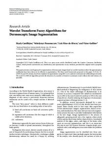
Type-1 Fuzzy Sets (T1FSs)
Let X be a universe of discourse and x be the elements contained in it. In a classical set A, an element x ∈ X may belong or not belong to the set A (refer to Figure 2.1). The membership function (MF) of a classical set A can be defined as:
1 if x ∈ X µA (x) = 0 if x ∈ /X
(2.1)
where µA (x) represents the membership grade.
Membership Grade
1 0.8 0.6 0.4 0.2 0 0
1
2
3
4
5
6
7
8
9
x
Figure 2.1: Classical Set with two values “0” & “1”.
Unlike a classical set, a fuzzy set expresses the degree to which an element x of X belong to a set. Hence in a T1FS A, each element has a crisp degree of MF in the interval between 0 and 1, and can be written as: µA (x) : X → [0, 1]
(2.2)
If the value of membership, µA (x), is restricted to either 0 or 1, then A is reduced to a 17
classical set. A T1FS, A, in terms of a single variable can be expressed as: A = {(x, µA (x))|
∀x ∈ X}
(2.3)
A can also be written as Z A=
µA (x)/x
(2.4)
x∈X
where
R
denotes union over all admissible x. A T1 Gaussian MF is required to be
between 0 and 1 for all x ∈ X and can be seen in Figure 2.2 . The T1 fuzzy MF does not contain any uncertainty as for each input data point there exist a crisp fuzzy membership value.
1
µ(x)
0.8 0.6 0.4 0.2 0 0
1
2
3
4
5
6
7
8
9
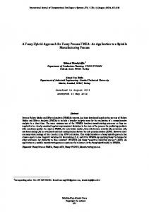
x(input) Figure 2.2: Gaussian type-1 fuzzy MFs [Mendel, 2001].
There are different types of type-1 MFs available in literature, each having different parameter sets. There is no unique choice of the shape of MFs for a specific problem and the shapes of MFs are mostly determined by trial and error. However, the one with less parameters providing good performance should be used. The commonly used MFs are: 18
1. Triangular MF: depends on three parameters a,b,c and can be described in a compact form as: � � x−a c−x µA (x; a, b, c) = max min( , ), 0 b−a c−b
(2.5)
2. Trapezoidal MF: depends on four parameters a,b,c,d and can be expressed in a compact form as: µA (x; a, b, c, d) = max {min[(x − a)/(b − a), 1, (d − x)/(d − c)], 0}
(2.6)
3. Generalized bell MF: depends on three parameters a,b,c and can be given as: � µA (x; a, b, c) = 1/ 1 + [(x − c)/a]2b
(2.7)
4. Gaussian MF depends on two parameters σ, c and can be described as: � µA (x; σ, c) = exp −[(x − c)2 /(2σ 2 )]
(2.8)
Type-1 fuzzy triangular, trapezoidal, generalized-bell and gaussian MFs with their associated parameters can be seen in Figure 2.3. Where the horizontal axis represents the domain in the range between 0 and 9, and the vertical axis represents the membership values in the range between 0 and 1.
19
(a) Type−1 Triangular MF
(b) Type−1 Trapizoidal MF
1 µ(x)
µ(x)
1
0.5
0 0
a
xi
b (c) Type−1 Generalized Bell MF
c
0 0
9
a
xi
b (d) Type−1 Gaussian MF
c
d
9
1 µ(x)
1 µ(x)
0.5
0.5
0.5
a
0 0
xi
σ c
0 0
9
xi
c
9
Figure 2.3: Type-1 fuzzy set with different MFs [Jang and Sun, 1997].
2.2.2
Type-1 Fuzzy Sets Operations
In FS theory, the operations of FSs can be defined in terms of their MFs. Let FSs A and B be described by their membership grade µA (x) and µB (x). The fuzzy union of these FSs A and B can be defined using maximum operator as [Mendel, 2001]: µA∪B (x) = max[µA (x), µB (x)]
(2.9)
while the fuzzy intersection of these FSs A and B can be defined using minimum operator as: µA∩B (x) = min[µA (x), µB (x)]
(2.10)
and using product operator as: µA?B (x) = prod[µA (x), µB (x)] = µA (x) ? µB (x) 20
(2.11)
The generalized form of fuzzy union is known as T-conorm. The most common Tconorm used in the FSs is the maximum operator max(a, b). Similarly, the generalized form of fuzzy intersection is known as T-norm and is usually minimum operator min(a, b).
2.2.3
Type-1 Fuzzy Logic System (T1FLS)
A type-1 fuzzy logic system (T1FLS) uses T1FSs theory to map crisp inputs to output. The crisp values of inputs are converted into fuzzy values during the fuzzification process based on the rules in the rule base. Fuzzy decisions are made in the inference part after which the output is converted into a crisp value during the defuzzification process. A T1FLS consists of four main parts namely fuzzifier, rule base, inference engine and a defuzzifier. Figure 2.4 illustrates the general block diagram of a T1FLS.
2.2.3.1
Fuzzifier
Fuzzifier takes the crisp inputs x = (x1 , x2 , . . . , xn ) in the universe of discourse X , and convert them into a T1FS , A, by assigning the degree of MF µAi (xi ) to each input in an interval between 0 and 1. Various MFs along different parameters are defined mathematically. The performance of a FLS can be improved by tuning the parameters of the MFs. 21
Crisp Input
Rules Fuzzifier
Fuzzy input set
Defuzzifier Inference
Crisp Output
Fuzzy output set
Figure 2.4: Type-1 fuzzy logic system block diagram [Mendel, 2001].
2.2.3.2
Rule base
A fuzzy rule base is a set of finite number of rules used for decision making. The rules can be acquired from experts’ knowledge or using data driven methods [Castro et al., 1999, Chen and Linkens, 2004]. A fuzzy rule is in the form of IF-THEN conditional statements. The IF part (known as antecedents) needs to be satisfied in order to infer the THEN part (known as consequents). Some examples of fuzzy rules in linguistic terms are as follows: • IF pressure is high THEN volume is high • IF age is young THEN experience is limited • IF height is tall THEN weight is heavy
2.2.3.3
Inference
The inference engine operates on T1FSs by evaluating the rules in the rule base. The fuzzy decision is made by using the fuzzy operations of union and intersection to produce fuzzy outputs in the form of T1FSs. 22
2.2.3.4
Defuzzification
The fuzzy outputs produced by the inference engine are translated into crisp output. This process is called defuzzification, as it is an inverse transformation of the fuzzification process. Among many defuzzifiers available in literature, a computationally simple defuzzifier is the criteria for selection. Such defuzzifiers include maximum, centroid, center-of-sums and mean-of-maxima.
2.3
Type-2 Fuzzy Sets and Systems
2.3.1
Uncertainty and Fuzzy Sets
Information deficiencies such as incomplete, fragmentary, not fully reliable, vague and contradictory information [Klir and Wierman, 1999] results in uncertainties in data and a process. Three types of uncertainties recognized and divided into two major classes in [Klir and Wierman, 1999] are 1. Fuzziness (or vagueness, cloudiness, unclearness) results from the imprecise boundaries of fuzzy sets. 2. Ambiguity i Nonspecificity (or impression, diversity) is linked with sizes of relevant sets of alternatives. ii Strife (or discrepancy, discord) expresses conflicts among the various sets of alternatives. Eight sources of uncertainties in FLSs are identified in [Khanesar et al., 2011a] are: 1. Precision of the measurement devices 2. Noise on the measurement devices 23
3. Environmental conditions of the measurement devices 4. Unknown nonlinear characteristics of the actuators 5. A real-time system cannot be modeled accurately, and there are always some modeling uncertainties. 6. The meaning of the words that are used in the antecedents and consequents of rules can be uncertain (words mean different things to different people) [Mendel, 2001] 7. Consequent may have a histogram of values associated with them, especially when knowledge is extracted from a group of experts who do not all agree [Mendel, 2001] 8. Uncertainties caused by some unvisited data that the FLS does not have predefined rules for T1FLS can only handle the uncertainties that are associated with the meaning of the words by using precise MFs. The choice of T1FLS is not appropriate in the presence of other sources of uncertainties in the real world data as it may cause problem in determining the exact and precise parameters of both the antecedents and consequents [Hagras, 2007]. The type-2 FLS however, can handle all type of uncertainties with their fuzzy grades [Mendel, 2001][p. 66–78]. Some of the advantages of type-2 FSs over T1FSs have been summarized by Hagras [Hagras, 2007] as: 1. Type-2 FSs with fuzzy MFs can handle the linguistic and numerical uncertainties more precisely than the T1FSs, as they have fuzzy MFs. 2. Presence of FOU in the type-2 FSs can cover the wider range, hence reduces the rule base as compared to T1FSs. 3. A large number of T1FSs are embedded in type-2 FSs that describe the variables with a detailed description adding extra levels of smooth control surface and response.
24
4. The extra degrees of freedom provided by the FOU enables a type-2 FLS to produce outputs that can not be achieved by T1FLSs with the same number of MFs.
2.3.2
Type-2 Fuzzy Sets (T2FSs)
The T2FSs are described by MFs that are characterized by more parameters than the T1FSs. As defined by Mendel and John [Mendel and John, 2002] a T2FS, denoted ˜ is characterized by a T2 fuzzy MF µ ˜ (x, u), where x ∈ X and u ∈ Jx ⊆ [0, 1]. by A, A Mathematically A˜ can be defined as [Mendel and John, 2002]:
A˜ = {((x, u), µA˜ (x, u))|
∀x ∈ X
∀u ∈ Jx ⊆ [0, 1]}
(2.12)
where µA˜ (x, u) is in 0 ≤ µA˜ (x, u) ≤ 1. A˜ can also be expressed as [Mendel and John, 2002]: A˜ =
Z
µA˜ (x, u)/(x, u) x∈X
where
RR
Z Jx ⊆ [0, 1]
(2.13)
u∈Jx
denotes union over all admissible x and u [Mendel and John, 2002].
Jx is called primary membership of x [Mendel and John, 2002]. Moreover, corresponding to each primary membership, there is a secondary membership that defines the possibilities for the primary membership. The secondary membership of a T2 fuzzy MF can be written as: Z µA˜ (x) =
fx (u)/(u)
Jx ⊆ [0, 1]
(2.14)
u∈Jx
where fx (u) are the secondary membership grade of x ∈ [0, 1]. In the general type-2 FLS, the secondary MFs can take values in the interval between 0 and 1. T2FSs would be a preferable choice in uncertain circumstance when the precise MFs can not be determined through crisp numbers. The Gaussian T2 fuzzy MF in Figure 2.5 illustrates that there is no crisp value for a specific x. 25
1
µ(x)
0.8
0.6 Upper MFs
0.4
0.2
FOU Lower MFs
0 0
0.1
0.2
0.3
0.4
0.5
0.6
0.7
0.8
0.9
1
x Figure 2.5: Gaussian T2 fuzzy MF (FOU) [Mendel and John, 2002].
FOU is a term given to the union of the primary memberships [Mendel and John, 2002], is limited by lower and upper MFs in T2FSs. Uncertainty in T2FS A˜ is characterized by FOU and can be written as: ˜ = F OU (A)
[
[µA˜ (x), µA˜ (x)]
(2.15)
x∈X
where µA˜ (x) and µA˜ (x) are the lower and upper MFs respectively. Fig 2.6 depicts the FOUs of triangular, trapezoidal, Gaussian and generalized bell MFs. 26
(a)Type−2 Triangular MF
(b) Type−2 Trapizoidal MF
1
1
0.8
0.8
0.6
0.6
0.4
0.4
0.2
0.2
0 −10
−5
0
5
10
(c) Type−2 Generalized Bell MF
0 −10
1
1
0.8
0.8
0.6
0.6
0.4
0.4
0.2
0.2
0 −10
−5
0
5
10
0 −10
−5
0
5
10
0
5
10
(d) Type−2 Gaussian MF
−5
Figure 2.6: Type-2 fuzzy set with different MFs.
2.3.3
Interval Type-2 Fuzzy Sets (IT2FSs)
When all the secondary MFs, µA˜ (x, u), of the T2FSs A˜ are equal to 1, then A˜ becomes an IT2FS. The IT2FS as a special case of (2.13) can be defined as: A˜ =
Z
Z 1/(x, u)
x∈X
Jx ⊆ [0, 1]
(2.16)
u∈Jx
T2FSs are computationally demanding because of the extra dimension. However, IT2FSs are more manageable as all points in the third dimension are at unity and can be ignored for modelling purposes [Mendel et al., 2006]. Additionally, dealing with IT2FS is comparatively easy than T2FS because they can be derived using T1 fuzzy mathematics [Mendel et al., 2006]. From the transition of type-1 to type-2 FLS, it is perceived that a general type-2 FLS should always outperform the interval type-2 FLS, which in turn should always outperform the T1FLS. However, the actual performance of a fuzzy system depends on the choice of model parameters as well as the variability of the uncertainty within the application [Wagner and Hagras, 2010b]. 27
2.3.4
Type-2 Fuzzy Sets Operations
T2FSs operations based on Zadeh extension principle [Zadeh, 1975] can be derived ˜ be the as in [Mizumoto and Tanaka, 1976, Karnik and Mendel, 2001b]. Let A˜ and B two FSs in the universe of discourse X and, µA˜ (x) and µB˜ (x) are their membership R R grades, respectively, where µA˜ (x) = u fx (u)/u and µB˜ (x) = w gx (w)/w while the primary membership of x are u, w ∈ Jx , Jx ⊆ [0, 1] and secondary membership grades of x are fx (u), gx (w) ∈ [0, 1]. The union and intersection of the T2FSs can be defined as [Mizumoto and Tanaka, 1976, Karnik and Mendel, 2001b]: ˜ ⇔ µ ˜ ˜ (x) = µ ˜ (x) t µ ˜ (x) = A˜ ∪ B A∪B A B
Z Z u
˜ ⇔ µ ˜ ˜ (x) = µ ˜ (x) u µ ˜ (x) = A˜ ∩ B B A A∩B
(fx (u) ? gx (w))/(u ⊗ w)
(2.17)
(fx (u) ? gx (w))/(u ? w)
(2.18)
w
Z Z u
w
where ⊗ represents the max t-conorm, which is the join operation in T2FSs and is denoted by t. Simialrly, ? represents a t-norm, which is the meet operation in T2FSs and is denoted by u. A complete method to calculate the meet and join operations of T2FSs are given in [Karnik and Mendel, 2001b].
2.3.5
Type-2 Fuzzy Logic Systems (T2FLS)
The structure of a T2FLS is the same as T1FLS except the defuzzifier block where it is replaced by an output processing block. The output processing block in T2FLS comprises of an additional component called the type-reducer followed by a defuzzifier block as shown in Fig 2.7. Because of the distinct nature of T2 fuzzy MFs, the output from the inference engine is T2FS. Since the defuzzifier can only input the T1FSs to produce crisp output therefore a type reducer is needed after the inference engine in the T2FLS to obtain a type-reduced set. This type-reduced set can be then defuzzified to crisp output. 28
Crisp Inputs
Rules
Defuzzifier
Crisp Output
Fuzzifier Type-1 FSs Type-2 FSs
Inference
Type-2 FSs
Type-reducer
Figure 2.7: Block diagram of T2FLS [Karnik et al., 1999].
2.3.6
Interval Type-2 Fuzzy Logic System (IT2FLS)
In general, it is very complicated to calculate the meet operation. A simplified version is introduced as IT2FLS. The meet and join operations in IT2FLS are performed with IT2FSs and are easy to compute as compared to T2FLS. In IT2FLS, the fuzzy inference, type-reduction and defuzzification processes deals with the interval sets rather than fuzzy and hence, only two end-point computations are needed. The research of this thesis is mainly focused on IT2FLS.
2.4
Takagi-Sugeno-Kang Fuzzy Logic System The two different kinds of FLS in literature are Mamdani fuzzy model [Mamdani,
1974] and Takagi-Sugeno-Kang (TSK) fuzzy model [Takagi and Sugeno, 1985]. The former is designed based on expert knowledge that uses linguistic variables in the fuzzy rules and uses the defuzzification process to get crisp output from fuzzy output [Hamam and Georganas, 2008]. However, the later is a model-based design where the rules are represented by a function of input variables [Cordon et al., 2001a] and the crisp output is generated using weighted average [Hamam and Georganas, 2008]. Since in this thesis we are using TSK model, this model is discussed. 29
2.4.1
Type-1 Takagi-Sugeno-Kang Fuzzy Logic System
A type-1 Takagi-Sugeno-Kang FLS (T1 TSK FLS) can be described by fuzzy IFTHEN rules. A first-order T1 TSK fuzzy model is the most common one [Mendel, 2001] and can be expressed as follows: Rk : IF x1 is Ak1 and x2 is Ak2 and · · · and xd is Akd THEN k
y =
ck0
+
ck1 x1
+ ··· +
ckd xd , =
ck0
+
d X
cki xi
(2.19)
i=1
where x1 , x2 , · · · , xd are the input variable, y k are the output variables and Aki are T1 antecedent FSs for kth rule and ith input. The parameters in the consequent part of the rules are c0 and cki (k = 1, · · · M, i = 1, · · · , d). The final output of the system can be written as:
PM
y = Pk=1 M
f k yk
k=1
(2.20)
fk
where f k are the rule firing levels, defined as: f k (x) = µAk1 (x1 ) ∗ · · · ∗ µAkd (xd )
(2.21)
in which ∗ denotes a t-norm and is usually a minimum or a product operator.
2.4.2
Type-2 Takagi-Sugeno-Kang Fuzzy Logic System
A T2 TSK FLS can also be described by fuzzy IF-THEN rules. A general first-order T2 TSK fuzzy model with a rules base of M rules can be expressed as: ˜ k : IF x1 is A˜k and x2 is A˜k and · · · and xd is A˜k R 1 2 d THEN Y k = C0k + C1k x1 + · · · + Cdk xd , = C0k +
Pd
i=1
Cik xi
where x1 , x2 , · · · , xd are the input variable, Y k is the output variable, A˜ki are T2FS 30
for kth rule and ith input. The parameters in the consequent part of the rules are C0 and Cik (k = 1, · · · M, i = 1, · · · , d) that are T1FSs. The final output of the T2 TSK fuzzy model is as follows: 1
Y (Y , · · · , Y
M
1
M
Z
Z
,F ,··· ,F ) =
Z
Z
··· y 1 ∈Y 1
··· y M ∈Y M
f 1 ∈F 1
f M ∈F M
M [Tk=1 µY k (y k )
,P
M µF k (f k )] ?Tk=1
M k k k=1 f y PM k k=1 f
(2.22)
where y k ∈ Y k , f k ∈ F k , M is the number of rules fired and T and ? are the t-norms. F k is the firing strength which is defined as: F k = µA˜k1 (x1 ) u µA˜k2 (x2 ) u · · · u µA˜k (xd ) d
(2.23)
where u represents the meet operation. This model is also known as A2-C1, where “A” and “C” are short for antecedent and consequent, respectively. This indicates that the antecedent part of this T2 TSK fuzzy model is T2FSs and the consequents part is T1FSs. Two other models of T2 TSK FLS are A2-C0 and A1-C1 that are summarized in Table 2.1 Table 2.1: Summary of T2 TSK FLS. Interval TSK FLS[%] A2-C1 A2-C0 A1-C1 Antecedent T2FS T2FS T1FS Consequent T1FS crisp number T1FS
2.4.3
Interval Type-2 Takagi-Sugeno-Kang Fuzzy Logic System
The Equation 2.22 involves complex computation and is therefore difficult to compute. In IT2FLS, the IT2FS are used for the antecedents and the IT1FS are used for the consequent sets of a T2 TSK rule then µA˜ki (xi ) and Cik are also an interval set and can be given as: 31
i = 1, · · · , d
µA˜ki (xi ) = [µA˜k (xi ), µ ¯A˜ki (xi )]
(2.24)
i
and Cik = [cki − ski , cki + ski ]
(2.25)
where cki represents the center and ski denotes the spread of Cik (k = 1, · · · , M ) and (i = 0, 1, · · · , d). With interval sets the Equation 2.22 simplifies to:
···
=
y M ∈[ylM ,yrM ]
y 1 ∈[yl1 ,yr1 ]
Y = [yl , yr ] ,P M k k k=1 f y ··· 1 PM k f 1 ∈[f 1 ,f¯1 ] f M ∈[f M ,f¯M ] k=1 f
Z
Z
Z
Z
(2.26)
where the indexes l and r in the IT2FSs, [yl , yr ], represent the left and right limits, respectively. f k and f¯k are the upper and lower firing set and can be expressed as [Liang and Mendel, 2000, Mendel, 2001]:
F k (x) = [f k (x), f¯k (x)]
(2.27)
where k
f (x) = µA˜k (x1 ) ? µA˜k (x2 ) ? · · · ? µA˜k (xd ) = 1
2
d
d Y i=1
and f¯k (x) = µA˜k1 (x1 ) ? µA˜k2 (x2 ) ? · · · ? µA˜k (xd ) =
d Y
d
µA˜k (xi )
(2.28)
µA˜ki (xi )
(2.29)
i
i=1
The output of the THEN-part (consequents part)of the kth rule is a crisp value that can be written as: k
w =
ck0
+
ck1 x1
+ ··· +
ckd xd , =
d X
cki xi ,
x0 , 1.
(2.30)
i=0
A T2 reducer then computes the interval FS [yl , yr ] using Z
Z
Z
···
[yl , yr ] = w1
Z ···
wM
f 1 ∈[f 1 ,f¯1 ]
1 f M ∈[f M ,f¯M ]
32
,P
M k k k=1 f w P M k k=1 f
(2.31)
The indices l and r in the interval FS, [yl , yr ], represent the left and right limits, respectively. There is no direct theoretical solution for the (2.31) and can be computed iteratively using the Karnik-Mendel (K-M) iterative model [Karnik and Mendel, 2001b]. In this model the consequent part parameters are usually reordered in ascending order. Assume w = [w1 , · · · , wM ]T as the original rule-ordered consequent values, and ˜ = [w˜ 1 , · · · , w˜ M ]T as the reordered consequent values, where w˜ 1 ≤ w˜ 2 ≤ · · · ≤ w˜ M , w ˜ according to [Mendel, 2004, Juang et al., 2010, Deng the association between w and w et al., 2014] can be given as ˜ = Qw w
(2.32)
where Q is a M × M permutation matrix that uses elementary vectors (vector, all of whose elements are zero except one unit element in a specified position) as columns. The elementary vectors in Q are arranged by relocating elements in w and arranging ˜ Details about the construction of them in ascending order in the transformed vector w. Q can be seen in [Mendel, 2004]. Accordingly, rearranging the rule-orders f k and f¯k k in ascending order and calling them f˜ and f¯˜k , respectively. The outputs y and y in l
r
Equation 2.31 can be computed as under [Mendel, 2004]: P ˜k ˜ k f¯˜k w˜ k + M k=L+1 f w PL ¯˜k PM k f˜ f +
(2.33)
P k ¯˜k ˜ k f˜ w˜ k + M k=R+1 f w PR ˜k PM f + f¯˜k
(2.34)
PL yl =
k=1
k=L+1
k=1
PR yr =
k=1
k=1
k=R+1
where L and R denote the left and right crossover points, respectively. These two points can be obtained using the K-M model [Karnik and Mendel, 2001b]. The defuzzified output of the interval set [yl , yr ], can be computed by taking the average of yl and yr . Hence, the defuzzified output is given by y=
yl + yr 2
33
(2.35)
2.5
Learning algorithms of Type-2 Fuzzy Logic System in Existing Literature
Since the inception of the fuzzy set theory in 1965, the mathematical advancements have progressed to exceptionally high standards. A plethora of research has been conducted on fuzzy systems and its implementations in many disciplines. A demanding analysis is required to collect the information on fuzzy system i.e, the theoretical and real-time applications of fuzzy sets available in literature. A literature review is conducted here through searching of bibliographic databases. The search is limited to four databases and to the years 2000-2014, respectively. These databases include IEEE Xplore, SpringerLink, ScienceDirect and Wiley online library. These four databases are the major publishers in the field of fuzzy logic theory. Initially, the term “fuzzy system” was searched. The search for this term identified papers in every aspect of the field such as; control system, modeling, design, theorem, expert system, knowledge, regression and classification. A total of 98,702 conference publications and 55,715 journal publications are searched using the above term. The search is then refined by the term “type-2 fuzzy”, using the query of hfuzzy systemi AND htype-2 fuzzyi, leaving away the publications in type-1 fuzzy logic theory. The annual number of publications for type-1 and type-2 fuzzy logic theory can be seen in Figure 2.8a. The large number of publications reported for type-1 fuzzy theory is due to the fact that the early introduced type-1 fuzzy logic systems (FLSs) have several software packages that simplify the task of researchers. However, a continuous increase in publication of type-2 FLSs (T2FLSs) can be seen in Fig 2.8b. The search is again refined by the query hfuzzy systemi AND hfuzzy learningi to pick the publications on fuzzy learning models only, which is also the main research focus of this study. Figure 2.9 shows the trend in the number of publications on fuzzy learning which shows the wider interest in adaptive fuzzy logic systems rather than conventional fuzzy logic systems. 34
(a)
Number of Publications
16000 8000
Type−2 Fuzzy Type−1 Fuzzy
0 (b)
400 200 0 2000
Type−2 Conference Type−2 Journal
2002
2004
2006
2008
2010
2012
2014
Year Figure 2.8: (a) Annual number of publications for type-1 and type-2 fuzzy logic theory, (b) Annual number of conference and journal publications for type2 fuzzy logic theory.
Number of Publications
16000 Fuzzy Learning Fuzzy System
14000 12000 10000 8000 6000 4000 2000 0 2000
2002
2004
2006
2008
2010
2012
2014
Year Figure 2.9: The annual number of publication on fuzzy learning.
The learning and tuning can be used interchangeably in the design of a FLS. However, the difference between the two is that the former is a process in FLSs where the search does not depend on predefined parameters, and automatic design of a FLS starts from the scratch, whereas the later starts the optimization of a FLS with a set of predefined parameters and focuses to find the best set. The fuzzy logic implementations are greatly widen with the addition of the concept of evolving modeling approaches. Evolving models are permanently updating their knowledge and understanding about diverse complex relationships and dependencies in real world application scenarios by integrating new system behaviors and environmental influences. A fuzzy system can 35
be extended to a new system by evolving its core components such as rules, antecedent fuzzy sets, inference and defuzzification methods. The main goal of the adaptive fuzzy systems is to enhance the predictive ability and usability [Alcala et al., 1999]. In addition to different parameter update rules, it is even possible to change the model itself which lead to evolving fuzzy systems which will not be focused in this paper. Different approaches of soft computing can be applied here to enhance the computational and predictive performance of fuzzy systems. Indeed, research has demonstrated that formalizing an issue pertaining human expert knowledge is a difficult and time consuming job. More often than not, it does not even prompt completely fulfilling results. For that reason, a sort of data-driven approach of fuzzy systems is usually beneficial [Alcala et al., 1999]. Generally, a fuzzy system with learning ability allows its different parameters to be tuned. The dashed arrow crossing the blocks of a T2FLS in Figure 2.10 shows the possible components to be tuned. During the design of a non-adaptive fuzzy system, the experts assign the linguistic labels to the problem variables by using fuzzy membership functions (MFs). However they cannot give the precise MFs defining the semantics of these labels. Normally, these values are defined by partitioning the domain of interest. Through discretization, the variables in the domain are partitioned into the equivalent number of intervals that of linguistic labels considered. The process needs to define a uniform fuzzy partition with symmetric and identical shape fuzzy sets. However, this approach generally ends up with a sub-optimal performance of the fuzzy system [Alcala et al., 1999]. In order to address this as a specific end goal, different learning techniques have been reported in literature for the generation of fuzzy set automatically. These techniques include decision tree [Kbir et al., 2000, Myles and Brown, 2003, Wang and Lee, 2006], clustering [Bezdek, 1981,Wang et al., 2013], hybrid models [Devillez et al., 2002, Yang et al., 2008, Li et al., 2009] and evolutionary algorithms [Cordon et al., 2000, Maulik and Bandyopadhyay, 2003, Acosta et al., 2007]. The presence of 3D-MF in T2FLS necessitates the adjustment of more parameters than T1FLS, which makes the learning process more complicated [hung Lee et al., 2003]. The footprint of uncertainty (FOU) in interval T2FLSs (IT2FLS) can also be tuned to improve the performance in the presence of noise [Hosseini et al., 2012]. 36
Crisp Inputs
Rules Fuzzifier
Defuzzifier
Inference
Crisp Output
Type-reducer
Figure 2.10: Learning parts of a T2FLS.
In general, fuzzy modeling is a system modeling with fuzzy rule based systems (FRBS) that represents a local model which is effectively interpretable and analyzable [Cordon et al., 2001a]. When the expert is not available or does not have sufficient information to stipulate the fuzzy rules, then numerical information is utilized to determine these rules. Two distinguished fusions of fuzzy with neural networks also known as neuro-fuzzy models [Hayashi and Buckley, 1994] and with genetic algorithm known as genetic fuzzy systems [Cordon et al., 2001a] have been used to automatically generate the fuzzy rules. FRBS is a universal approximator as it can approximate any function to the desired degree of accuracy [Kosko, 1994, Castro, 1995]. FRBS is a preferable choice over neural networks (NN), as the parameters involved have a real world meaning and consequently the initial guess parameters can substantially enhance the training algorithm. The optimization methods for FLS can be broadly categorized into three methods as shown in Fig 2.11. • Derivative-based (computational approaches), • Derivative-free (heuristic methods), • Hybrid methods which are the fusion of both the derivative-free and derivativebased methods. 37
Derivative-based Back-propagation Levenberg-Marquardt
Derivative-free Genetic algorithm
Hybrid-Learning Derivativebased
Particle swarm optimization Back-propagation + Kalman filter
Kalman filter
Ant colony optimization
Least square
Artificial bee colony
Radial basis function
Simulated Annealing
Simplex method
Sliding mode theory
Gradient descent + Kalman filter
Extreme learning machine
Others
Ordinary least squares + Backpropagation
Other combinations Particle swarm optimization + Gradient descent Particle swarm optimization + Least squares Genetic algorithm + Kalman filter
Figure 2.11: Different learning methods for T2FLS.
2.5.1
Derivative-Based or Gradient Descent-Based Learning Algorithms
The objective of the methods listed in this category is to solve nonlinear optimization problems through an objective function by using derivative information. Some of the derivative-based, also known as Gradient-based optimization, methods are discussed below particularly for T2FLS and IT2FLS.
2.5.1.1
Back-Propagation Algorithms
Back-propagation (BP), also known as steepest-descent or gradient descent (GD), algorithm is one of the most popular techniques used to update the parameters a T2FLS. In [Mendel, 2004] the mathematical formulation and computational flowcharts for computing the derivatives have been provided that are needed to implement the steepestdescent algorithm to tune the parameters of T2FLSs. In order to adjust the parameters 38
of a T2FLS, this algorithm needs to compute the first derivatives of the objective function with respect to every single parameter. The main body of the paper has focused on IT2FLSs. A challenging task of deriving the derivatives of the BP algorithm is taken for the antecedent and consequent parameters of the IT2FLS. FOU selection was prolonged so as to make the results appropriate to all sort of FOU. In the last part, the type of MFs for IT2FLS was specified keeping in mind the end goal to finish the computations. Center-of-set type-reduction was replaced by the two end-points of the centroid to reduce the number of design parameters. IT2FLS design with GD method is usually used for benchmark purposes. The fusion of NNs and T2FLS results in a novel structure, type-2 fuzzy neural network (T2FNN), which was presented by Wang et al. in [Wang et al., 2004] to handle uncertainty with dynamical optimal learning. A T2FNN consists of a T2 fuzzy linguistic process as the antecedent part, and the two-layer interval NN as the consequent part. In order to simplify the computational process, interval T2FNN was adopted. The training algorithm of the antecedent and consequent parameters in interval T2FNN was derived using a GD. GA is combined with the dynamical optimal training algorithm to determine the optimal spread and learning rate for the antecedent part of interval T2FNN. The proposed model outperformed T1FNN in several examples. However, the fuzzy rule reordering problem while computing the left and right end points were not properly derived with the parameters learning equations. The issue is highlighted and a complete and detailed version of the specific BP equations were derived in [Hagras, 2006] to tune both the antecedent and consequent parameters of the interval T2FNN.
2.5.1.2
Levenberg-Marquardt Algorithm
Keeping in mind that the performance might be improved if higher derivatives instead of first derivatives are used, Khanesar et al. proposed a T2FNN based on Levenberg-Marquardt algorithm [Khanesar et al., 2011b]. The algorithm uses second order derivatives that made the training process faster. A simple method of computation of the Jacoboan matrix which is being the most difficult step in implementing the 39
Levenberg-Marquardt algorithm was also described. A modified version of the novel T2 fuzzy MF with certain values on both ends of the support and the kernel, and some uncertain values on the other values of the support (Elliptic MF) [Khanesar et al., 2010] was also proposed. The proposed learning algorithm in T2FNN is utilized for the prediction of a Mackey-Glass time series data. The effectiveness of the proposed algorithm was shown with the benchmark GD algorithm. The Levenberg-Marquardt algorithm was also utilized by Castillo et al. in [Castillo et al., 2013] for optimizing the parameters of an adaptive IT2FNN. The universal approximation of the IT2FNN was shown based on Stone-Weierstrass theorem as major contribution of the paper. Simulation results of nonlinear function identification using the proposed IT2FNN for different number of variables with the Mackey-Glass time series data has been presented.
2.5.1.3
Kalman filter-based Algorithm
Khanesar et al. proposed the use of decoupled extended Kalman filter for the optimization of both the parameters of the antecedent and consequent parts of T2FLS [Khanesar et al., 2012]. By utilizing the decoupled extended Kalman filter, certain group of parameters had interaction between groups instead of one group that minimized the computational cost. A novel T2 fuzzy MF having certain values on both ends of the support and the kernel, and uncertain values on other parts of the support were taken to benefit the T2FLS. Comparison of the models was conducted with a population based particle swarm optimization and with a first-order GD-based method for the optimization of the antecedent part of T2FLS. The proposed T2FLS structure was tested on different noisy data set, that have illustrated better performance of extended Kalman filter based method over the benchmark models. Moreover, noise rejection characteristics of the novel T2 fuzzy MF was shown in the simulation results. The impact of inaccurate statistics on the obtained results of a noise-sensitive Kalman 40
filter is avoided by an adaptive Kalman filter based design of an IT2 fuzzy logic system [Hua et al., 2015]. Based on the proportion of the actual value of the residual covariance to its theoretical value, the proposed model dynamically adjusted the measurement noise covariance. The adjustment changed the values of the filter to improve the accuracy of the state estimation. The proposed method was validated by conducting extensive simulations with respect to the position estimation of ship. The simulation results were compared with a standard Kalman filter based T2FLS (where adaptive techniques was not utilized) and with an adaptive Kalman filter based T1FLS.
2.5.1.4
Least Square Method
A regression model for IT2 fuzzy sets based on the least squares estimation technique was presented by Poleshchuk and Komarov in [Poleshchuk and Komarov, 2012]. Unknown coefficients were assumed to be triangular fuzzy numbers. Aggregation intervals for T1 fuzzy sets were determined whose lower and upper MFs were of IT2 fuzzy sets. These aggregation intervals were called weighted intervals. The IT2 fuzzy MFs for the developed regression models were taken of type piecewise linear functions. The standard deviation, hybrid correlation coefficient, and hybrid standard error of estimates were defined for reliability evaluation.
2.5.1.5
Radial Basis Function
The IT2 fuzzy membership functions from labeled pattern data and its application to radial basis function networks (RBFN) was presented by Rhee and Choi in [Rhee and Choi, 2007]. The authors constructed the histogram of the sample data for each labeled class and feature by smoothing the domain of each feature by a symmetric window function (e.g., a triangular function). The vertex of the triangular function was positioned at the first bin of the histogram and the weighted moving average was calculated, then the vertex was moved to the next bin. This procedure was repeated for all of the bins. The histogram was fitted by a 4th degree polynomial function to determine the number and 41
approximate parameter values for a IT2 fuzzy Gaussian MF. T1 fuzzy MFs, which were computed from the centroid of the IT2 fuzzy MFs, were incorporated into the RBFN. The proposed MF assignment was shown to improve the classification performance of the RBFN since the uncertainty of pattern data were desirably controlled by IT2 fuzzy MFs. A new robust controller based on the integration of a RBFN and an IT2 fuzzy logic controller for robot manipulator actuated by pneumatic artificial muscles was proposed by Amar et al. in [Amar et al., 2012]. The proposed approach was synthesized for each joint using sliding mode control (SMC) and named RBFN T2 fuzzy sliding mode control. Avoiding difficult modeling, attenuating the chattering effect of the SMC, reducing the rules number of the fuzzy control, guaranteeing the stability and the robustness of the system, and handling the uncertainties of the system were highlighted as some of the objectives that can be accomplished using this control scheme. The proposed control approach was synthesized and the stability of the robot using this controller was analyzed using Lyapunov theory. The efficiency of the proposed controller was compared with other control technique. The superiority of the proposed controller compared to a RBFN T1 fuzzy SMC were demonstrated from results. Finally, an experimental study of the proposed approach was presented using 2-DOF robot.
2.5.1.6
Simplex Method
A modified IT2 TSK FLS was proposed by Wang et al. in [Wang et al., 2011]. First, the T1 TSK FLS was built using subtractive clustering method combined with least square method. The T2 TSK FLS was then obtained from the T1 TSK FLS through unconstrained optimization using the Nelder-Mead Simplex method by varying the parameters of the antecedent and consequences. The modified IT2 TSK FLS was applied to a heat exchange process on the equipment CE117 Process Trainer. The efficiency of the proposed Simplex method for IT2 TSK FLS over T1 TSK FLS was demonstrated during experiment. 42
The T2 fuzzy linear programming problems was solved in [Dinagar and Anbalagan, 2011] by using two-phase simplex method. A new ranking function for T2 fuzzy sets was defined using graded mean integration representation. Original objective function for fuzzy linear programming was defined during the first phase. The simplex method was employed in phase 2 to find the optimal solution to the original problem. The two phase method, using the proposed new ranking function as linear ranking functions on T2 fuzzy numbers, appeared to be natural extension of the results for linear programming problem with crisp data. The authors suggested that the capabilities offered may be useful for post optimal analysis.
2.5.1.7
Extreme Learning Machine
An efficient T2 fuzzy extreme learning algorithm was proposed for training IT2 TSK FLS [Deng et al., 2014] based on extreme learning machine strategy. In the proposed algorithm, the parameters of the antecedent part were generated randomly and the parameters of the consequent part were obtained using the extreme learning mechanism. The performance of the proposed algorithm was evaluated with three existing learning algorithms of the IT2FLS on various synthetic and real-world data sets. Results demonstrated highly competitive generalization performance among other algorithms.
2.5.2
Derivative-free or Gradient free Learning Algorithms
In the conditions that the derivative information is unavailable, unreliable or unfeasible, derivative-free methods are preferred. These methods do not need functional derivative information to search a set of parameters that minimize (or maximize) a given objective function. Rather, they depend solely on repeated evaluation of the objective function [Jang and Sun, 1997]. Derivative-free optimization has encountered a restored enthusiasm over the previous decade that has energized another influx of theory and algorithms. Automatic design of T1FLS using such optimization algorithms has become a standard practice. The trend has now transferred to automatic design of T2FLS and 43
IT2FLS using these algorithms. A concise review on some of such optimization algorithms for T2FLS has been done in [Castillo and Melin, 2012b]. Reference [Castillo et al., 2012] presented a comparative study of bio-inspired algorithms applied to optimization of T1 and T2 fuzzy logic controller (FLC). Below are some of the derivativefree optimization methods that have been utilized for optimizing T2FLS.
2.5.2.1
Genetic Algorithm
Genetic algorithm (GA) is an adaptive heuristic search algorithm based on a formalization of natural selection and genetics. The basic principles of GAs were first proposed by John Holland in 1975, inspired by the mechanism of natural selection, where stronger individuals are likely the winners in a competing environment [Cordon et al., 2001a]. A population of chromosomes, objective function and stopping criteria are required to be defined in GA. The population then undergoes genetic operation to evolve and the best population is selected based on the objective function. In order to optimize a T2FLS by means of GA, it must be represented as a population of chromosomes. A diverse applications using GAs for T2FLS optimization has been overviewed in [Castillo and Melin, 2012c]. A designing method for a T2FLS using GA was proposed by Park and Kwang in [Park and Lee-Kwang, 2001]. The positions and the shapes of the MFs and the rules of a T2FLS were determined through the proposed method.T2 fuzzy parameters in T2FLS were encoded as chromosome. The proposed method is applied to the chaotic time-series prediction and the result of the experiment is shown to demonstrate the performance. GA was also proposed for the optimization of a T2FNN [hung Lee et al., 2003]. The feature parameters to represent a T2 fuzzy set were determined first, then using these parameters, a T2FNN system was encoded as a chromosome. The real-code GA was then used to optimize the T2FNN antecedent and consequent MFs. Wu and Tan [Wu and Tan, 2006a] utilized GA for designing a T2FLS to control 44
non-linear plants presented performance evaluation of interval T2FLC using GA. This paper focuses on advancing the understanding of interval T2FLC. The T2FLC was then compared with another three GA evolved T1FLCs that have different design parameters. The objective was to examine the amount by which the extra degrees of freedom provided by antecedent T2 fuzzy sets are able to improve the control performance. Experimental results show that better control can be achieved using a T2FLC with fewer fuzzy sets/rules so one benefit of T2FLC is a lower trade-off between modeling accuracy and interpretability. The design methodology IT2FNN was introduced by Park et al. in [Park et al., 2009] to optimize the network using a real-coded GA. The antecedent part was comprised of the fuzzy division of input space and the consequent part of the network was represented by polynomial functions. The parameters of the network were optimized using GA. The proposed network was evaluated with the chaotic Mackey-Glass time series data and NOx emission process data of gas turbine power plant. Forecasting comparison of IT2FNN with T1FNN proved better performance of the proposed model. The high capability of T2FLSs in combination with the GA for managing the uncertainty issues inherited in the inputs of a computer aided detection (CAD) system classifier was studied by Hosseini et al. in [Hosseini et al., 2010]. Additionally the paper also presented an optimized genetic IT2FLS with Gaussian MFs approach for a multidimensional pattern recognition problem with a high number of inputs. Furthermore, the GA is employed for tuning of the MFs parameters and FOU. In order to assess the performance, the designed IT2FLSs are applied on a lung CAD application for classification of nodules and was compared to T1FLS. The results reveal that the Genetic IT2FLS classifier outperforms the equivalent T1FLS and is capable of capturing more uncertainties. An optimization method for the design of T2FLS based on the FOU of the MFs using GA was proposed by Hidalgo et al. in [Hidalgo et al., 2012]. Three different cases were considered to reduce the complexity problem of searching the parameter space of solutions. T2 fuzzy MFs optimized using GA were considered in different cases for changing the level of uncertainty of the MF so as to achieve the optimal solution at the 45
end. The improvement of the designed method over T1FLS was evidenced on three benchmark problems. A new system of T2 genetic fuzzy system was proposed by Shukla and Tripathi in [Shukla and Tripathi, 2014]. A genetic tuning approach named lateral displacement and expansion/compression in which α and β parameters were calculated to adjust the parameters of IT2 fuzzy MFs. The system considered the interpretability and accuracy features during its design. It was concluded that the proposed tuning approach is interpretable and the experimental results were found satisfactory. The T2FNN MFs are optimized using GA and PSO in [Gaxiola et al., 2016]. The T2FNN was optimized in a way to obtain the T2 fuzzy weights while maintaining the structure of two inputs, one output and the six rules structure. The resulting optimized T2FNN is applied to the Mackey-Glass time series data prediction. The advantage of the optimized fuzzy weights of T2FNN using GA and PSO was illustrated over T2FNN having non-optimized T2 fuzzy weights. The superiority of the results of the optimized models are also proved with statistical analysis.
2.5.2.2
Particle Swarm Optimization
Particle swarm optimization (PSO) is a population-based stochastic optimization technique developed by Eberhart and Kennedy in 1995 [Eberhart and Kennedy, 1995]. Inspired by the behavior of a population of moving individual particularly, bird flocking and fish schooling, the PSO looks for the best solution. The agents in PSO are called particles. A function or system must be represented as a particle when using a PSO for optimization. The advantages of using the PSO optimization technique for automating the design process of T2FLS has also been illustrated in [Castillo and Melin, 2012d]. A training method for a T2FLS using PSO was presented by Al-Jaafreh and AlJumaily in [Al-Jaafreh and Al-Jumaily, 2007]. T2FLS and PSO were utilized together, the procedure to analyse the problem was explained and finally presented a new method 46
to optimize parameters of the primary MFs of T2FLS using PSO to improve the performance and increase the accuracy of the T2FLS. The proposed optimization method is implemented on mean blood pressure estimation. The heart rate was input to the system using five Gaussian MFs. The PSO was utilized to adjust the parameters of MFs to minimize the difference between the actual and obtained mean blood pressure. A satisfactory performance of the proposed method was observed during the analysis of the results. A T2FNN optimized using PSO as a reliable on-site partial discharge pattern recognition algorithm was developed by Kim et al. in [Kim et al., 2009]. T2FNNs exploit T2 fuzzy sets which are robust in the diverse area of intelligence systems. Considering the on-site situation where it is not easy to obtain voltage phases to be used for phase resolved partial discharge analysis, the partial discharge data sets measured in the laboratory were artificially changed into data sets with shifted voltage phases and added noise in order to test the proposed algorithm. The results obtained by the proposed algorithm were compared with that of conventional NN and the RBFN. The proposed T2FNNs appeared to have better performance when compared to conventional NN. The design and simulation of T2 fuzzy MFs for the average approximation of an interval of T2FLC was proposed using PSO [Maldonado et al., 2013]. In order to reduce the runtime of the algorithm, some points of triangular and trapezoidal T2 fuzzy MFs were considered for modifications using optimization and, the consequent parameters were not altered. Three objective functions namely overshoot, undershoot and steady state error were considered for the performance ability of the T2FLC. The proposed controller was applied on FPGA implementation and the results were compared with the same controller optimized using GA under uncertainty.
2.5.2.3
Ant Colony Optimization
Ant colony optimization (ACO), a meta-heuristic algorithm, is motivated by the behavior of ants in discovering paths from their colony to the food source [Cordon et al., 47
2001a]. The technique can be utilized for issues that can be reduced to discovering the superior paths along graphs. By optimizing T2FLS with ACO, it should be represented as one of the paths that the ants can follow in a graph. The advantages of using the ACO optimization techniques for automating T2FLSs were briefly reviewed in [Castillo and Melin, 2012a]. A Reinforcement Self- Organizing IT2FLS with ACO was proposed by Juang et al. in [Juang et al., 2009]. In order to improve system robustness to noise, the IT2 fuzzy sets were used in the antecedent part whereas ACO was utilized to design the consequent part of each fuzzy rule. The consequent part was selected from a set of candidate actions according to ant pheromone trails. The proposed model was applied to a truck backing control. Comparison of the proposed model was done with reinforcement T1FLS to verify its efficiency and effectiveness. The results of the comparison verified the robustness of the proposed model to noise. A new reinforcement-learning method using online rule generation and Q-valueaided ACO for an IT2FLS based controller was proposed by Juang et al. in [Juang and Hsu, 2009]. The antecedent part in the IT2FLS utilized IT2 fuzzy sets to enhance the controller robustness to noise. The structure and parameters of an IT2FLS were simultaneously designed in the proposed method. An online IT2 rule generation method for the evolution of system structure and flexible partitioning of the input space was proposed. Consequent part parameters in an IT2FLS were designed using Q-values and the reinforcement local-global ACO algorithm. The consequent part was selected from a set of candidate actions according to ant pheromone trails and Q-values, both of which were modified using reinforcement signals. The proposed method was applied to the truck-backing control, magnetic-levitation control, and a chaotic-system control. In order to verify the efficiency and effectiveness of the proposed mode it was compared with other reinforcement-learning methods . Comparisons with T1FLS verify the robustness property of using an IT2FLS in the presence of noise. Optimization of the MFs of an IT2FLC using ACO and PSO for an autonomous wheeled mobile robot were presented by Castillo et al. in [Castillo et al., 2012]. Statistical comparison of the optimization model was examined in detail with one another 48
and with a GA based IT2FLS, so as to determine the best optimization method for this specific mechanical autonomy issue. During comparison, it was observed that both PSO and ACO had the capacity to beat GAs for this specific application. However, in a comparison between ACO and PSO, the best results were accomplished with ACO. In this case, the authors concluded that ACO is the most appropriate optimization algorithm for this robotic problem. A T2FLS with a defuzzifier block determined through ACO as an optimal intelligent controller was proposed by Rezoug et al. in [Rezoug et al., 2014]. The optimized T2FLC was exploited under an unmanned aerial vehicle. The performance of the ACO based T2FLC was compared with a PSO based T2FLC applied to Birotor helicopter system. The superiority and the effectiveness of the proposed method was illustrated over the PSO based T2FLC and a classical T2FLC cases.
2.5.2.4
Bee Colony Optimization
The bee colony optimization (BCO) is also a meta-heuristic algorithm and is inspired by the foraging behavior of honeybees [Lucic and Teodorovic, 2003]. A bee in BCO represents an agent; and a FLS or FLC must be represented as a bee to optimize it using BCO. A new optimization technique for T1 and T2FLCs using the BCO was presented by Amador-Angulo and Castillo in [Amador-Angulo and Castillo, 2014]. The collective intelligent behavior that bees have for the solution of optimization problems was analyzed for T1 and T2FLCs. The optimization of the MF parameters of T1 and T2FLC was made using BCO and was applied to a benchmark problem of water tank controller. The fuzzy controllers were analyzed with different variants of the design. Better result was obtained with T2FLC when noise was applied in a T2FLC. 49
2.5.2.5
Simulated Annealing
An optimized design of IT2FLS was presented using simulated annealing (SA) by Almaraashi et al. in [Almaraashi and John, 2011]. The parameters of the antecedent and the consequent parts of the IT2FLS were optimized using SA by minimizing the objective function. The optimized model was then applied to predict the Mackey-Glass time series by searching for the best configuration of the IT2FLS. By using an adaptive step size for each input during Markov chain, the SA reduced the computation time of IT2FLS. The results of the proposed methodology were compared to that of a T2FLS. A general T2FLS was designed using SA algorithm with the aid of an IT2FLS [Almaraashi et al., 2012]. The focus of the proposed was to reduce the computations needed to get the best FOU using IT2FLS. The proposed methodology consists of three stages, i.e., designing of IT2FLS using SA, conversion of IT2 fuzzy set into symmetrical general T2 fuzzy set and then learning of FOU of general T2FLS using SA. The methodology was applied to four bench-mark problems. The outcomes demonstrated that the conversion process conveyed a decent estimate to the IT2FLS outputs with little misfortunes in accuracies and reduces the computations.
2.5.2.6
Sliding Mode Theory
A SMC-theory-based learning algorithm was proposed to upgrade the rules for both the premise and consequent parts of a T2FNNs [Kayacan et al., 2015]. The algorithm also tuned the sharing of the lower and upper MFs of the T2FNN to deal with the varying uncertainties in the rule base of a T2FLS. Besides, the learning rate of the system was updated during the online training. The stability of the proposed learning algorithm has been verified by using an appropriate Lyapunov function. Faster convergence speed of the proposed algorithm had been demonstrated over the existing methods. 50
2.5.2.7
Others
The most influential fuzzy rules in the design of a T2FLS were determined with two novel indices for T2 fuzzy rule ranking presented by Zhou et al. in [Zhou et al., 2007]. These indices were named R-values and c-values of fuzzy rules separately. The estimation of the rank for the singular value decomposition and QR factorization with column pivoting algorithm was avoided by obtaining the R-values of T2 fuzzy rules that were obtained by applying QR decomposition. In order to perform the rule reduction, the c-values of T2 fuzzy rules were suggested to rank rules based on the effects of rule consequents. Experimental results on a signal recovery problem had shown that by using the proposed indices the most influential T2 fuzzy rules were identified and the parsimonious T2FLS was constructed effectively with satisfactory performance. IT2FLSs were optimized with two types of tabu search (TS) by Almaraashi and Hedar in [Almaraashi and Hedar, 2014]. The best configuration of the IT2FLS parameters was sought through TS. Directed TS, that uses pattern search to control TS moves, and short-term TS with IT2FLS were utilized and applied to a classification issue of two benchmark data sets. The focus of the paper was to improve the structure and lessen the computation time of IT2FLSs utilizing an intelligent directed search instead of a random search. The directed TS-based IT2FLS outperformed the default TS-based IT2FLS by a noticeable difference during comparison . This perception uncovered the significance of utilizing a guided search moves as opposed to utilizing a randomized search direction in IT2FLS. An IT2FLS was designed with the help of coevolutionary approach by Hostos et al. in [Hostos et al., 2011]. The number of MFs were kept fixed while that of rules were kept vary to inspect the performance of the IT2FLS. The evolutionary algorithm utilized these parameters to acquire an IT2FLS. The interpretability of the model was satisfied by setting up a constrained fuzzy partition for every input so as the coevolution process look for the best MFs within a constrained distribution. A T1FLS was designed with the same parameters as T2FLS for comparison purposes. Simulation results of a Mackey-Glass time series prediction proved the capability of the proposed IT2FLS 51
in achieving better results on the interest of few generations. However, this approach needs a greater computational burden. The novel application of Big BangBig Crunch optimization approach to optimize the antecedent parameters of the IT2 fuzzy PID controllers in a cascade control structure is presented in [Kumbasar and Hagras, 2014]. The Big BangBig Crunch is employed to tune the parameters of the IT2FLC as its computational cost is low and convergence speed is high. The proposed IT2 fuzzy PID is compared with its T1 fuzzy PID and conventional PID controller counterparts that are also optimized using Big BangBig Crunch method. The results illustrate that the proposed IT2 fuzzy PID greatly enhanced the control performance even in the presence of uncertainties and disturbances over other models. A fuzzy edge detector based on the Sobel technique and IT2FLS is optimized using cuckoo search and GA with the aim to determine the optimal antecedent parameters of the IT2FLS [Gonzalez et al., 2014]. The goal of using IT2FLS in edge detection methods was to provide them with the ability to handle uncertainty in processing real world images. Simulation results revealed that using an optimal IT2FLS in conjunction with the Sobel technique provides a powerful edge detection method that outperforms its type-1 counterparts and the pure original Sobel technique.
2.5.3
Hybrid Learning Algorithms
A combination of two or more models in a single model is known as a hybrid model. Hybrid models are becoming increasingly popular due to their synergy in performance. Hybrid learning algorithm are likewise a mix of more than one learning algorithms used in designing the optimized models to improve the performance of the models. These algorithms may be of same type i.e., derivative-based or derivative-free or may be a combination of both. 52
2.5.3.1
Derivative-based Hybrid Learning Algorithms
The issue of dealing with uncertain information was suggested with the development of new methods [Castro et al., 2009]. Three IT2FNN models as an integration of IT2 TSK FLS and adaptive NN, with hybrid learning algorithms were proposed to solve the issue. GD and GD with adaptive learning rate were used as a hybrid learning algorithm. Keeping in mind the end goal to fuzzify the antecedents and consequents rules of an IT2 TSK FLS; IT2FNN was utilizes at the antecedents layer and IT1FNN at the consequents layer. Experimental were conducted with a non-linear identification in control system and prediction of a noisy Mackey-Glass time series data. During the comparative analysis of the optimized IT2FNN and an adaptive neuro-fuzzy inference system, IT2FNN was demonstrated as a proficient mechanism for modeling real-world problems. A hybrid learning algorithm based on recursive Kalman filter and BP was presented for IT2 TSK FLS [Mendez et al., 2010]. The consequent parameters were tuned using recursive Kalman filter during the forward pass and antecedent parameters were tuned using BP algorithm. The IT2 TSK FLS with hybrid learning algorithm was implemented for temperature prediction of the transfer bar at hot strip mill. Comparison of the proposed model was done with the existing models in literature. Better performance of the model was demonstrated with the hybrid learning algorithm than the individual techniques when used alone for the same data sets. A TSK-based self-evolving compensatory IT2FNN was proposed for system modeling and noise cancellation problems [Lin et al., 2014] . The proposed model utilized T2 fuzzy set in a FNN to handle the uncertainties associated with information or data in the knowledge base. The antecedent part of each compensatory fuzzy rule was an IT2FS in the proposed model, where compensatory-based fuzzy reasoning utilized adaptive fuzzy operation of a neural fuzzy system to make the FLS effective and adaptive, and the consequent part was of the TSK type. The TSK-type consequent part was a linear combination of exogenous input variables. Initially, the rule base in the proposed model was empty. All rules were derived according to online T2 fuzzy clustering. For 53
parameter learning, the consequent part parameters were tuned by a variable-expansive Kalman filter algorithm to the reinforce parameter learning ability. The antecedent T2 fuzzy sets and compensatory weights were learnt by a GD algorithm to improve the learning performance. Performance of the proposed model for identification was validated and compared with several T1 and T2FNNs. Simulation results have shown that the proposed approach produced smaller errors and converges more quickly. A hybrid learning algorithm of orthogonal least-square (OLS) and BP method was used to tune the consequent and antecedent parameters of an interval singleton T2 TSK FLS, respectively [Gerardo M. Mendez and Rendon-Espinoza, 2014]. The proposed hybrid learning algorithm alters the parameters of IT2FLS adaptively. The model was compared with three other models with hybrid learning mechanism and the four models were applied to an industrial application. The proposed hybrid OLS-BP algorithm for IT2 TSK FLS outperformed the rest of the models.
2.5.3.2
Other Combinations of Hybrid Learning Algorithms
A self-evolving IT2FNN with online structure and parameter learning was proposed [Juang and Tsao, 2008]. In this model, the antecedent parts were IT2 fuzzy set and consequent part were of TSK type. The online clustering method was utilized initially to generate the fuzzy rules. The consequent parts were then tuned using the rule-ordered Kalman filter algorithm. The antecedent parts parameters were learnt through GA. The proposed self-evolving IT2FNN model was applied to simulations on nonlinear plant modeling, adaptive noise cancellation and chaotic signal prediction. Better performance of the self-evolving IT2FNN was verified in comparison with T1FLS and T2FLS. A novel T2 TSK NN that utilizes general T2 fuzzy set, was proposed for function approximation [Jeng et al., 2009]. The type reduction, structure identification, and parameter estimation were recognized as issues in developing a general T2FNN. The issue of type reduction was solved by utilizing the idea of α-cuts that decomposed a general 54
T2 fuzzy set into IT2 fuzzy set. The issue of structure identification was settled by combining the incremental similarity based fuzzy clustering and linear least squares regression. The fuzzy rules were then extracted from these clusters and regressors. The last issue of the antecedent and consequent parameters identification of general T2FNN was solved using a hybrid learning algorithm of PSO and recursive least squares. Two simulation experiments were conducted to check the performance of the proposed model. Performance of the general T2FNN was compared with that of T2FNN and IT2FNN. Robust performance of the general T2FNN was observed against outliers than the other models. A hybrid method consisting of PSO and GD algorithms was utilized to optimize the parameters of a T2FLS [Khanesar et al., 2010]. A diamond-shaped T2 fuzzy MF was introduced as a novel method of MF for T2FLS. The proposed method was then tested on the prediction of a noisy Mackey-Glass time series data. The performance of the models was compared with existing T2FLS. The simulation results has shown that the T2FLS with hybrid learning algorithm and novel MF outperformed the other models. A hybrid learning algorithm incorporating PSO and lease-square estimation was presented for T2FNN in [Yeh et al., ]. The structure of a T2FNN was identified using a self-constructing fuzzy clustering method. The antecedent and the consequent parameters of T2FNN were optimized using PSO and lease-square estimation, respectively. Comparison of the proposed model was done with two existing methods in literatures. The effectiveness of the proposed methodology was shown through several experiments. A PSO based integrated functional link IT2FLS was presented for the prediction of stock market indices [Chakravarty and Dash, 2012]. An integrated model of TSK model that employs T2 fuzzy sets in the antecedent parts and the outputs from the functional link artificial NN in the consequent parts was designed. The parameters of the hybrid model were optimized with BP and PSO independently. Forecasting ability of the proposed model is compared with T1FLS and local linear wavelet NN optimized with BP and PSO. Better performance of the proposed model for stock market indices forecasting was observed over the other designed models. 55
A hybrid heuristic algorithm using PSO and GAs for parameter optimization of IT2FLS was proposed in [S. and M., 2011]. The proposed system was then utilized for two benchmark data sets of classification problem. Comparison of the model based on proposed hybrid algorithm was done with the existing classifiers in literature. The proposed method was able to minimize the rule-base and linguistic variable, and produced an accurate classification at 95% with the Iris data set and 98.71 with the Wisconsin Breast Cancer data set. An optimal design of IT2 TSK FLS was proposed using a hybrid algorithm [Long and Meesad, 2014] . A hybrid of chaos firefly algorithm and GA was utilized to determine the optimal parameters of MFs and consequents parameters of the IT2 TSK FLS. The structure and number of fuzzy rules were determined through a fuzzy c-means clustering algorithm. The optimal design of IT2 TSK FLS was employed to predict sea water level in short-term and long-term horizontal. The performance of the hybrid algorithm of IT2 TSK FLS was compared with GA and firefly algorithm based optimal designs of IT2 TSK FLS. The hybrid algorithm for IT2 TSK FLS outperformed both the GA and firefly algorithm for sea water level prediction problem.
2.6
Extreme Learning Machine (ELM) Inspired by biological neural systems, the NN have been emerged as a powerful
computational tool, with potential utilization in forecasting, function approximation, classification, modeling and pattern recognition problems. Most NNs have some sort of training rules whereby the weights of connections are adjusted on the basis of data. A promising feature of NNs is its ability to learn from example providing a framework to the problems having no exact solution [Paplinski, ]. The conventional feed-forward NNs mainly utilized the BP and its variants to train the model. Although the NNs can achieved reasonable performance when trained by them, however these algorithms suffer from the issues like stopping criteria, learning rate, iterative learning and over tuning [Zhu et al., 2005, Huang et al., 2006b] that has pushed the researchers to forge new learning algorithms with efficient learning scheme. 56
Figure 2.12: Structure of ELM.
A new learning algorithm called extreme learning machine (ELM) was introduced by Huang et al. [Huang et al., 2006b], [Huang et al., 2006a] to solve the issues of conventional learning algorithms in single-hidden layer feed-forward NNs (SLFN). Instead of adjusting the network parameters iteratively, ELM selects the input weights and hidden neurons of SLFN randomly and determines the output weights of SLFN analytically. Being a unified learning algorithm with predominant feature mapping ELMs are increasingly utilized for classification and regression problems [Huang et al., 2012], [Zheng et al., 2013], [Luo et al., 2015]. The structure of ELM can be seen in Fig 2.12 and the basics of ELM as a learning algorithm for SLFNs is described as follows. T n For a given training sample {(xi , yi )}N i=1 , where xi = [xi1 , xi2 , · · · , xin ] ⊂ R and
˜ hidden nodes is modeled yi = [yi1 , yi2 , · · · , yim ]T ⊂ Rm , the output of ELM with N as [Zhang et al., 2015]:
yi,k =
˜ N X
βj g(wj · xi + bj ),
i = 1, · · · , N
j=1
k = 1, · · · , m 57
(2.36)
where βj,k = [βj1 , βj2 , · · · , βjm ] represents the weights connecting the output nodes and the jth hidden nodes, bj is the threshold of the jth hidden node, and wj · xi denotes the inner product of wj and xi . g(wj · xi + bj ) represents an active function of hidden nodes with parameters wj and bj . Equation (2.36) can be written as the following matrix form [Zhang et al., 2015]:
Hβ = Y,
(2.37)
where H(wj , bj , xi ) g(w1 · x1 + b1 ) · · · g(wN˜ · x1 + bN˜ ) .. .. ... = . . g(w1 · xN + b1 ) · · · g(wN˜ · xN + bN˜ ) ˜
(2.38)
N ×N
(2.39)
N ×m
β11 · · · β1m = · · · . . . · · · m 1 βN˜ · · · βN˜ ˜
(2.40)
N ×m
· · · y1m = · · · . . . · · · m 1 yN · · · yN
β T1 . β = .. β TN˜ ˜
N ×m
and
yT1 . Y = .. yTN
y11
N ×m
here H is the hidden layer output matrix of the network, Y is the target matrix, yT is the transpose of vector y, and β is the output weight matrix. The parameters wj and bj of the hidden nodes are generated randomly. The output matrix β need to be calculated, that can be determined analytically with the least squares solutions. An optimal solution βb of β under the constraint of minimum least square min k β k and min k Hβ − Y k β
58
β
of the linear system in (2.37) can be calculated as βb = H† Y
(2.41)
where H† is the Moore-Penrose generalized inverse of matrix H [Serre, 2002, Rao and Mitra, 1971].
2.6.1
Fuzzy-ELM
An online sequential extreme learning machine (OS-ELM) algorithm was proposed for SLFN with RBF nodes that can either learn a single or a block of data [Liang et al., 2006]. Based on the theory of ELM, the center and widths of the nodes were generated randomly and the output weights were determined analytically. The functional equivalence between RBF networks and FIS under some minor limitation [Jang and Sun, 1993] has led the beginning of integrating ELM and FIS. The possibility of applying ELM to a TSK fuzzy model (ETSK) was explored by Sun et al. [Sun et al., 2007]. With the development of online sequential fuzzy extreme learning machine (OS-FuzzyELM), Rong et al. [Rong et al., 2009] expanded the same concept further by verifying the functional equivalence between SLFN and FIS with any MF. Based on the analysis of relation between the two, an evolutionary fuzzy extreme learning machine (E-FELM) was proposed [Yanpeng Qu and Shen, 2011]. The E-FELM was applied to a challenging issue of mammographic risk analysis. In all the above fuzzy-ELM research works, the input weights were assigned randomly, and the output weights were determined analytically. In [Zhang and Ji, 2013], a new fuzzy ELM method was proposed to solve the imbalance and weighted classification problems. The proposed method provided a logical result than the conventional ELM. Incorporating principles of human meta-cognition in the original OS-Fuzzy-ELM, Yong et al. [Yong et al., 2014] proposed meta-cognitive FELM (McFELM) in order to make the learning more efficient. McFELM had two parts: the cognitive part and the meta-cognitive part. The cognitive part was a FELM which learn sequential data one at a time or in blocks, while the meta-cognitive part 59
controlled the learning process of the subjective part utilizing a self regulating mechanism to make different learning conclusions. An extreme learning adaptive neuro fuzzy inference system (ELANFIS) was proposed that combines the learning capabilities of NNs and the explicit knowledge of the FIS in the same manner as the conventional ANFIS does.
2.6.2
Optimal-ELM
The introduction of ELM has made a revolutionary change in the learning process by avoiding the issues of conventional learning algorithms such as stopping criteria, learning rate, learning epochs and local minima [Zhu et al., 2005]. However the random generation of the input nodes usually ends in the generation of a large model that may hinder its efficiency. Soon after this realization, the importance of optimal parameters for ELM in SLFN is reported. A hybrid of ELM and differential evolutionary algorithm was proposed to find the optimal input weights and hidden biases [Zhu et al., 2005]. An evolutionary ELM based on PSO was proposed by You and Yang in [Xu and Shu, 2006] to optimize the input weights and biases of the ELM. The input weights and hidden biases of an ELM were also optimized based on the bacterial foraging (BF) algorithm [Jae-Hoon Cho, 2007]. An incremental ELM (I-ELM) [Huang and Chen, 2008] was proposed that randomly add the hidden nodes one by one and freezes the output weights of the existing hidden nodes when a new hidden node is added. Enhanced I-ELM (EI-ELM ) [Huang and Chen, 2008], as an improved implementation of I-ELM, was proposed where the node having smallest residual error is selected as an optimal hidden node among several randomly generated hidden nodes. Other variants of ELM are convex I-ELM [Huang and Chen, 2007], error-minimized ELM (EM-ELM) [Feng et al., 2009], optimally pruning ELM (OP-ELM) [Miche et al., 2010], and bidirectional ELM (B-ELM) [Yang et al., 2012] that tried to reduces the number of hidden nodes during the training process without affecting the learning effectiveness of ELM. In these algorithms the optimal nodes were selected the ones with lower residual error among the several randomly generated 60
hidden nodes. The compactness and generalization capability of the ELM was improved by integrating ELM and leave-one-out(LOO) cross validation with a two-stage stepwise construction procedure [Deng et al., 2011]. Bayesian ELM (BELM) [Soria-Olivas et al., 2011] was proposed to optimize the weights of the output layer using probability distribution. An approach for the automated design of networks using an ELM with adaptive growth of hidden nodes (AG-ELM) was proposed [Zhang et al., 2012]. As opposed to I-ELM where the existing hidden nodes are frozen with the arrival of a new node, AGELM determined the size of the hidden layer adaptively so as to reduce the network size and achieve better generalization performance. The issue of manually selection of trial vector generation strategies and control parameters of differential evolution in E-ELM was solved with the development of a self-adaptive evolutionary ELM (SaE-ELM) [Cao et al., 2012] that optimized the network parameters by using the self-adaptive differential evolution. All these above algorithm have revealed the importance of optimal parameters of the ELM in a SLFN. However the hybrid model of fuzzy and ELM have not yet been reported with optimal parameters and are usually generated randomly. As there are chances that the randomly assigned parameters might not create suitable MF in fuzzy model and should be determined optimally.
2.7
Artificial Bee Colony Optimization Algorithm
The Artificial Bee Colony (ABC) algorithm is based on a bee swarm intelligent algorithm that simulates the foraging behavior of honey bees. ABC was first presented to solve the numerical optimization problem by Karaboga [Karaboga, 2005]. The population-based ABC algorithm consists of three groups of foraging bees: employed bees associated with specific food sources, onlooker bees watch the dance of employed bees to select a food source, and scout bees search for food sources randomly. The scout bees discover the food sources that are exploited by employed and onlooker bees 61
until exhausted. The employed bee whose food source has been exhausted becomes a scout bee and search for further food sources. In ABC algorithm, the position of a food source represents a possible solution to the problem to be optimized. The nectar amount of the food source corresponds to the quality of the food source. In the ABC algorithm, the bee colony is divided half into employed bees and onlooker bees. The number of employed bees is equal to the number of food sources around hive. Let xi = [xi1 , xi2 , · · · , xiM ], i = 1, 2, · · · , SN represents the ith food source in the population, where SN is the size of population and M is the number of optimization parameters. In otherwords, each food source xi (i = 1, 2, · · · , SN ) is a M-dimensional vector. ABC generates a randomly distributed initial population of SN solutions (food source positions) as: xij = xmin + rand(0, 1) · (xmax − xmin ) j j j
(2.42)
where xij is a parameter to be optimized, xmin and xmax are the lower and upper bounds j j of the jth parameters of the solution i. After the first stage, the population is subjected to repeated cycles of the three phases of the ABC: employed bee phase, onlooker bee phase and scout bee phase. The employed bee produces a modification on the position in her memory for finding a new food source. A candidate food source position is produced in ABC using the following expression: νij = xij + φij · (xij − xkj )
(2.43)
where k ∈ 1, 2, · · · , SN for k 6= i and j ∈ 1, 2, · · · , M are randomly chosen indexes and φij is a random number between [0, 1]. Based on the fitness value the employed bee perform greedy selection between the old and new food source positions. After completing the search process, the employed share the information about the position and quality of the food source to the onlooker bee. The onlooker bee picks a food source depending on the probability value pi of that food source which is calculated by the following expression: f iti pi = PSN n=1 f itn 62
(2.44)
where f iti represents the fitness of the ith solution in a population. The probability of a food source being selected by the onlooker bees increases as the fitness values of a food source increases. After the selection of the food source, the onlooker bee repeat the steps of employed bee and the food source having high fitness value is memorized. The pseudo-code of the ABC can be seen in Algorithms 1. Algorithm 1 Pseudo-code of the ABC 1: Set parameters of the algorithm. 2:
Initialize food source position randomly.
3:
Evaluate the fitness of the food source (nectar amount)
4:
cycle =1
5:
repeat
6:
Employed bees phase: Produce new solution νi using Eq (2.43) Evaluate the fitness f iti Apply greedy selection process
7:
Calculate the probability of each solution using Eq 2.44.
8:
Onlooker bees phase: Choose any solution xi based on probability pi Produce new solution νi Evaluate the fitness f iti Apply greedy selection process
9: 10: 11:
Scout bees phase if an abandoned solution exist then replace it with a new random solution using Eq 2.42
12:
end if
13:
Memorize the best solution achieved so far cycle=cycle+1
14:
until cycle=MaxCycle
15:
print best and stop. A recent survey of the advances with ABC and its applications [Karaboga et al.,
2014] has cited only two papers of the fuzzy optimization using ABC. Some recent works on fuzzy and ABC are reviewed here. Fuzzy MFs of a single-input single output 63
system were optimized using ABC [Turanoglu et al., 2011]. The proposed algorithm was compared with a PSO by taking the best among the 10 runs in one experiment and by varying the different parameters in another experiment. It was concluded that any can be used to determine the optimal MF in a fuzzy system. A novel version of Fuzzy C-Means clustering technique with variable string length ABC was utilized in the design of a fuzzy model [gang Su et al., 2012]. ABC was also utilized to design a fuzzy wavelet neural network (FWNN) in order to improve the accuracy of the function approximation and the general capability of the FWNN [Heidari et al., 2013]. The number of fuzzy rules containing wavelets were determined using OLS algorithm. The accuracy of function approximation and the general capability of the FWNN were improved in a self tuning process by utilizing the ABC algorithm. Better performance and faster convergence of the ABC was demonstrated against shuffled frog leaping algorithm. An optimal method for defuzzification for an IT2FLC was presented in [Allawi and Abdalla, 2014]. Instead of averaging the two extreme from the output of type-reducer, an ABC was employed to achieve the optimal values for defuzzification. MFs of T1 and T2FLC were optimized using a BCO in [Amador-Angulo and Castillo, 2014]. A new fuzzy time series method with optimization of the fuzzification block using ABC was proposed in [Egrioglu et al., 2014]. Design of fuzzy model based on ABC and a hybrid of ABC-LS was proposed in [Habbi and Boudouaoui, 2014]. In the first model, the ABC alone was used to optimize all the parameters of the fuzzy model. In the second modeling strategy, a hybrid of ABC and LS were utilized to optimize the premise and the consequent parameters of the fuzzy model, respectively. The effective performance of ABC as a new optimization tool for FLS motivated us to utilize it in a hybrid learning algorithm for IT2FLS.
64
2.8
Critical Analysis on Learning Algorithms of IT2FLS T2FLS have extensively been applied to various engineering problems, e.g. identi-
fication, prediction, control, pattern recognition, etc. in the past two decades, and the results were promising especially in the presence of significant uncertainties in the system. In the design of IT2FLS, the early applications were realized in a way that both the antecedent and consequent parameters were chosen by the designer with perhaps some inputs from some experts. Since 2000s, a huge number of papers have been published which are based on the adaptation of the parameters of IT2FLS using the training data either online or offline. Consequently, the major challenge was to design these systems in an optimal way in terms of their optimal structure and their corresponding optimal parameter update rules. This section compares and contrasts the optimization algorithms for the training of IT2FLS discussed in Section 2.5. Undoubtedly, each training method has its own pros and cons. We believe that a deep knowledge about the advantages and disadvantages of the training methods makes it possible to decide on an appropriate optimization method based on the problem to be solved.
65
66
Full Heuristic optimization approaches
[hung Lee et al., 2003, Castillo et al., 2012, Juang et al., 2009, Hidalgo et al., 2012, Almaraashi, 2012, Castillo and Melin, 2012c, Kim et al., 2009, Maldonado et al., 2013] Yes
No
Extreme Learning Machine
No
Sliding Mode theory based adaptation
[Deng et al., 2014]
No
Levenberg Marquardt
No
No
Gradient descent
Kalman filter
[Mendel, 2004, Castro et al., 2009] [Castillo et al., 2013, Khanesar and Kayacan, 2015] [Kayacan and Kaynak, 2012, Kayacan et al., 2015] [Khanesar et al., 2012, Hua et al., 2015]
References
Yes
Yes
Yes
Yes
No
No
Yes
No
Yes
Yes
Yes
Yes
Yes
Yes
No
Yes
No
No
Simple
Simple
Yes
Simple
Yes
Yes
High
Low
Low
Low
Low
Low
Table 2.2: Summary of the existing learning algorithms for type-2 fuzzy logic system. Optimality Algorithm Design Para. Closed form Complexity Time Antecedent Consequent
Low
High
High
High
High
High
local minima
67
Proposed
Hybrid Heuristic optimization and others
[Juang and Tsao, 2008, Castro et al., 2009, Mendez et al., 2010, Yeh et al., , Lin et al., 2014, Gerardo M. Mendez and RendonEspinoza, 2014, Long and Meesad, 2014, ChungTa Li and Lin, 2014, Kayacan and Khanesar, 2016]
Hybrid Heuristic optimization and Extreme Learning Machine
Algorithm
References
Yes
Yes
Yes
No
Yes
Yes
Table 2.2 Continued. Optimality Design Para. Antecedent Consequent
Yes
Yes
Closed form
Simple
Simple
Reasonable
Reasonable
Complexity Time
Low
Low
local minima
The derivative-based methods, which are also called the computational methods, need some partial derivatives to be computed in order to update the parameters of the T2FLS. The use of the derivatives of the output of the system with respect to its parameters gives a mathematical moving direction for the parameters of T2FLS. The parameters of the T2FLS may either appear linearly and nonlinearly in its output [Kayacan et al., 2015]. The derivatives of the output of the fuzzy system with respect to the parameters which appear linearly in the output can be easily calculated. Moreover, least square, recursive least square and Kalman filter and its variants are proven be optimal estimators for these parameters [Mendel, 2004, Castillo et al., 2013, Khanesar et al., 2012] . However, the calculation of the partial derivative of the output of T2FLS with respect to the parameters of the antecedent part is difficult and does not have any explicit form . As these parameters appear in both numerator and the denumerator of the fuzzy rules; it is hard to calculate the derivative of output with respect to the parameters of the antecedent part [Kayacan and Ahmadieh, 2016]. This makes the implementation of the computational methods difficult for the antecedent part parameters. In addition, none of computational methods are optimal for updating the parameters of the antecedent part . There are certain parameters in the derivative-based algorithms that need to tuned manually during the design of IT2FLS e.g., while applying the Kalman filter for the consequent part, proper selection of noise covariance matrices (Q and R) is needed [Khanesar et al., 2012]. However, it may sometimes become difficult to get optimal parameters specially for R. Another drawback of these methods is that they cannot always provide a closed form solution to the problem [Sang, 2008]. Entrapment in local minima is another disadvantage of these methods [Kayacan and Ahmadieh, 2016]. Using computational methods, we may face stability issues as well. For instance, in gradient method too large learning rate may cause divergence. In Kalman filter, the covariance matrix may result in divergence and so on. There are also some other disadvantages which are not common for all computational methods and are restricted to one or two algorithms. For example, in extended Kalman filter the size of covariance matrix is very large when it is used to train the parameters of T2FLS. In Levenberg-Marquardt algorithm, the inverse of a large size matrix is required in each step [Roweis, 1996]. In summary, when the parameter search space is too big, these methods start suffering
68
from matrix manipulations. The derivative-free or heuristic optimization methods are another class of optimization methods which have been successfully applied to the optimal design of T2FLS [Juang et al., 2009, Hidalgo et al., 2012, Castillo et al., 2012, Castillo and Melin, 2012b, Castillo and Melin, 2012a, Maldonado et al., 2013]. The main advantage of these methods is that they are easy to implement and no mathematical update rule is needed to find the next step in the adaptation process of the parameters. Moreover, since they benefit from multiple initial points, the possibility of entrapment of these algorithms in local minima is much less than computational methods. However, since these algorithms are random optimization methods the update process is totally random and even if the values of the parameters are near their optimum values there is no guarantee that in the next step the error becomes less. Another drawback of these algorithms is that they necessitate the huge number of the evaluation of the T2FLS which is generally very slow and time-consuming and generally are recommended for offline problems. Memory requirements may also be another disadvantage of these methods. The hybrid learning algorithms for IT2FLS benefit from both heuristic and derivative based methods. The consequent part parameters appear linearly in the output of the FLS that is why the derivative based methods to optimize the parameters of the consequent part are easy to implement. Moreover, these methods benefit from some mathematics and usually converge much faster than random optimization methods and hence they are a preferable choice for the training of these parameters. In addition, some of derivative based methods e.g. Kalman filter and recursive least square are proven to be optimal for the parameters which appear linearly in the output of the FLS. However for the optimization of the premise part parameters since they appear nonlinearly in the output, it is quite probable that these parameters trap in local minima and random optimization techniques may be more preferable choices in these cases. The advantage of hybrid learning algorithms with respect to the derivative-based methods is that, the hybrid learning algorithm are much simpler to implement. Since there exists a normalization layer in the structure of neuro-fuzzy systems when one wants to take the partial derivative of output with respect to the antecedent part parameters all of the
69
rules have all of the parameters of the antecedent part even in the numerator or in the denumerator. This makes the derivative-based methods too hard to be implemented. However, since hybrid learning algorithm benefit from heuristic approaches it is much simpler to implement. Moreover, hybrid learning algorithms benefit from a closed form that can ease their implementation. Furthermore, the derivative-based methods suffer from instability and possibility to entrap in a local minima. Although hybrid learning algorithms are easier to implement and it is less probable for them to trap in a local minima, they are slower to be executed with respect to the derivative-based methods as multiple evaluation of the structure of the IT2FLS is needed. In comparison between hybrid learning algorithms and full heuristic approaches to train the IT2FLS such as PSO, GA etc., it must be said that since ELM for the consequent part is already optimal, use of heuristic for this part imposes tremendous amount of computation which are not necessary and seldom results in outcomes close to the optimal points found by ELM. Even if they become close to the results obtained by ELM, they never find the exact values found by ELM. Hence, full heuristic approaches take a lot of time and may not be exact enough. A concise review of bio-inspired algorithms for the design of IT2FLS for particular application was presented [Castillo and Melin, 2012b]. PSO, GA and ACO were utilized to find the optimal parameters of the membership functions of the IT2FLCs. In their conclusion, they suggested the use of ABC for the antecedent part parameters of the IT2FLS. Better performance of ABC over other algorithms was presented in a comparative study of ABC, GA, PSO, differential evolution algorithm and evolution strategies [Karaboga and Akay, 2009]. From all these analysis, it is deduced to use two hybrid learning algorithms based on heuristic algorithms and ELM for the design of IT2FLS.
2.9
Summary This chapter presented the theory, models and learning algorithms of the fuzzy sys-
tems. First part of the chapter introduced fuzzy sets and FLS followed by T2FLS. IT2FLSs are then discussed as a simplified version of T2FLS. The issue of uncertainty 70
has also been discussed in this art. The major challenge which has been paid much attention in this field during the last two decades is “how to optimally design these systems in terms of their optimal structure and their corresponding value of the parameters”?. This chapter identified and reviewed three major classes of optimization methods that are : derivative or computational approaches, derivative free or heuristic methods and hybrid methods which benefit from both the aforementioned approaches. A review of the current state of the art in different optimization methods as applied to deal with this challenging problem has been done. Each of the training methods has its own benefits and suffers from some draw backs. Knowledge about the advantages and disadvantages of the training methods makes it possible to decide on an appropriate optimization method based on the problem to be solved. The theory of ELM is also explained, followed by its hybrid model with fuzzy system. The chapter also discussed the issue of optimal parameters for ELM. In next chapter, the methodology of the design of IT2FLS using hybrid learning algorithms is described in detail.
71
72
CHAPTER 3 METHODOLOGY
The major challenge in the design of interval type-2 fuzzy logic system is to determine the optimal parameters for their antecedent and consequent parts. This chapter presents the design of interval type-2 fuzzy logic system using two hybrid learning algorithms to analyze and forecast nonlinear dynamic systems. First hybrid learning algorithm is the combination of extreme learning machine and genetic algorithm, where the parameters of the consequent part are tuned using extreme learning machine and the parameters of the antecedent part are optimized using the genetic algorithm, respectively. The second hybrid learning algorithm utilizes the hybridization of extreme learning machine and artificial bee colony optimization algorithm to tune the parameters of the consequent and antecedent parts of the interval type-2 fuzzy logic system, respectively. Starting from the determination of the chaotic behavior in data, data preprocessing, model design, validation and verification all are parts of this chapter. The organization of the chapter is as follows. Section 3.1 presents the justification of using hybrid of extreme learning machine (ELM) with genetic algorithm (GA) and artificial bee colony optimization algorithm (ABC). Section illustrates the framework for this research. Section 3.3 describes the procedure of tuning the parameters of the consequent part of the IT2FLS using ELM. Optimization of the antecedent part parameters of T2FLS using genetic algorithm and artificial bee colony optimization are presented in Section 3.4 and 3.5. Model verification is discussed in Section 3.6 and summary of the chapter is given in Section 3.7.
73
3.1
Discussion and Rationale for Choice of Approach From the literature review, it is noticed that almost all part of a FLS can be optimize,
but the main emphasis is given to the optimization of the fuzzy inference. A fuzzy inference in a form if-then rules is a system consists of MFs in the antecedent part and the weights in the consequent part [Abraham, 2005]. NNs is one of the simplest methods used to determine the fuzzy inference system (FIS) [Hayashi and Buckley, 1994, Lu, 2011]. However in the hybrid neuro-fuzzy model there is no guarantee of the convergence or the efficacy of the tuning of the FIS. The inconvenience caused by the NNs in tuning the FIS was tackled by using the natural intelligence of the evolutionary computation [Abraham, 2005]. The general interaction of the evolutionary search for the FIS is illustrated in Figure 3.1. The Optimization of the FIS using evolutionary learning algorithms is at the top on the slow scale and optimization of the antecedent part is at a faster time scale than that of consequent part. Various hybrid learning algorithms for Slow
Search of fuzzy inference system Search of fuzzy rules (consequent part)
Search of membership functions (antecedent part)
Fast
Time scale
Figure 3.1: Optimization of the fuzzy inference system with the interaction of evolutionary algorithms. the design of IT2FLS have been proposed to improve the performance of the system. An IT2FNN with support vector machine (SVM) has optimized the network parameters with higher generalization capability [Juang et al., 2010]. However, to solve the quadratic programming problems, the computational time of the SVM based IT2FNN remained high. Although the training accuracy of SVM is better, however, they take much time in training. Additionally, some algorithms such as GD tend to cause overfitness shows that it has a bad generalization. Moreover, they are notorious for being susceptible to local minima. Furthermore, an IT2FLS tuned using KF provides good 74
accuracy but the KF requires the R (the covariance of measurement noise) parameter to be tuned by trial and error. The tuning of parameters of IT2FLS using these algorithms will therefore be very time consuming. In the recent years, ELM has emerged as one of the most efficient intelligent learning algorithms. The rigorous proof of universal approximation of ELM with much milder conditions has already been provided [Huang et al., 2006a, Huang et al., 2006b, Huang and Chen, 2008]. Extensive comparisons of different learning algorithms like GD, SVM, ELM and self evolving IT2 FLS/NN have been carried out in [Deng et al., 2014] for various data sets. Better generalization ability and computational time of the ELM based IT2FNN was observed over other algorithms. This indicates that unlike the conventional learning algorithms, ELM tends to achieve both the smallest training error and the smallest norm of output weights [Huang et al., 2006a] in less training time. The traditional learning algorithms are usually very slow and require iterative tuning of the parameters to achieve high learning performance. ELM is an emerging learning technique which trains the system without iterative tuning [Huang et al., 2006b, Huang et al., 2006a]. The other motivation for using ELM in the consequent part is that the IT2FLS tuned using traditional learning algorithms cannot cope with the increasing size of data sets due to its high computational demand. This may restrict the broad utilization of IT2FLS, as big data sets are getting to be the real source of information in the design of IT2FLS for real world applications. Although the hybrid learning algorithms are more complex in design and may have longer search time than the single one, they are less likely to entrap in a local minima and they can be designed to be optimal for the consequent part parameters. As discussed in Chapter 2, the hybrid learning algorithms benefit from both the heuristic and derivative based methods. The consequent part parameters appear linearly in the output of the fuzzy system that is why the derivative based methods to optimize the parameters of the consequent part are easy to implement. However, for the optimization of the premise part parameters since they appear nonlinearly in the output, it is quite probable that these parameters trap in local minima and random optimization
75
techniques may be more preferable choices in these cases. In addition, they can benefit from the faster time scale when optimize using these algorithms. In this fashion, the hybrid learning algorithms for IT2FLS benefit from the strong capability of heuristic methods to search the whole space and the mathematics behind the computational methods which boosts the optimization and lessen the probability of searching inappropriate areas. A concise review of bio-inspired algorithms for the design of IT2FLS for particular application was presented [Castillo and Melin, 2012b]. PSO, GA and ACO were utilized to find the optimal parameters of the membership functions of the IT2FLCs. The use of these algorithms had already become a standard practice in the design of T1FLS. The review also concluded that hybrid learning algorithms combining different bio-inspired optimization techniques could be good alternatives for the optimization of T2FLSs. Among other algorithms, ABC optimization was also suggested to be utilized for the optimization of T2FLSs. Since GA is the simplest method used for the optimization of the antecedent part parameters, therefore, it is hybridized with the ELM in the first hybrid learning algorithms of the IT2FLS. Where the consequent part parameters are tuned using ELM and the antecedent parameters are optimized using GA. We call this algorithm GA-IT2FELM. Once the effective performance is achieved from the GA-IT2FELM, it is decided to apply more sophisticated algorithms to obtain the optimal parameters for the IT2FLS. Based on the suggestion of the utilization of ABC for the optimization of T2FLS [Castillo and Melin, 2012b] and better performance of ABC over other algorithms presented in a comparative study of ABC, GA, PSO, differential evolution algorithm and evolution strategies [Karaboga and Akay, 2009], a combination of ABC and ELM is selected in the second hybrid learning algorithm so as to achieve the optimal parameters of the IT2FLS. The consequent part parameters in this hybrid learning algorithms are tuned using ELM and the antecedent part parameters are optimized using ABC. The algorithm is named as ABC-IT2FELM.
76
3.2
Research Framework Hybrid learning algorithm in an interesting topic where two or more algorithms
are combined to solve the optimization problems. Design of the IT2FLS using hybrid learning algorithm is an interesting research area. Hybrid learning algorithms for IT2FLS may be a combination of derivative-based [Castro et al., 2009, Mendez et al., 2010, Maldonado et al., 2013, Lin et al., 2014, Gerardo M. Mendez and RendonEspinoza, 2014], derivative-free [S. and M., 2011,Long and Meesad, 2014] or combination of both [Khanesar et al., 2010,Yeh et al., ]. Figure 3.2 show the research framework for the design of IT2FLS using hybrid learning algorithms. The research framework comprises of eight major steps: (1) selection of structure of the IT2 TSK FLS, (2) literature Survey is done to determine suitable algorithms that can be hybridized for the design of IT2FLS, (3) select data having chaotic behavior. (4) Data preprocessing is done to normalize the data and then the normalized data is divided into training and testing data-sets. (5) Optimization of the IT2FLS is performed such that the consequent part parameters are tuned using ELM and the antecedent part parameters are optimized using heuristic approaches. (6) Performance assessment of the proposed hybrid learning algorithms of IT2FLS are conducted using performance matrics. (7) Next the antecedent part parameters are generated using three different design approaches. (8) Finally, comparisons are performed to evaluates the accuracy of the proposed design of IT2FLS.
77
Structure of the Fuzzy Logic System
Interval Type-2 Takag-Sugeno-Kang Fuzzy Logic System (IT2 TSK FLS) Literature Survey
Investigation of suitable algorithms for Hybrid learning algorithms of IT2 TSK FLS Select Data
Determine chaos in data Data Preprocessing
Training and Testing data-sets Optimization of IT2 TSk FLS
Encoding of Antecedent part parameters in GA/ABC
Antecedent parameters
Training of the Consequent parameters
Fine tuning of the Consequent parameters
Interval Type-2 Extreme Learning Machine (IT2FELM)
stopping criteria No achieved
Yes
No GA/ABC operations Forecasting
Performance Assessment
Accuracy testing using performance matrics Comparisons
Design approaches for the antecedent part parameters
Antecedent parameter generation of IT2FELM Manual construction
IT2FELM
Randomly generated
IT2FELM
Optimized
IT2FELM
Manual
Random
Optimal
Comparisons
Hybrid model of IT2FLS Models available in literature
Figure 3.2: Research framework for the design of IT2FLS using hybrid learning algorithms.
78
3.3
Optimization of Interval Type-2 Fuzzy Logic System using Extreme Learning Machine (IT2FELM) ELM is originally proposed for SLFN [Huang et al., 2006b]. From the functional
relationship between FLSs and NNs [Jang and Sun, 1993, Castro et al., 2002], it is observed that under some mild conditions FLSs can be interpreted as a special case of SLFN and can be trained using its learning algorithms. The ELM considers the fuzzy rules as hidden nodes of the SLFN [Rong et al., 2009]. Learning of the IT2FLS can be done using three steps of ELM (ref Fig 3.3) as under:
Initialize the antecedent parameters randomly
Initialize the consequent parameters
Tune the consequent parameters
Figure 3.3: Flowchart of IT2FELM. 1. Identification of the antecedent parameters. 2. Initialize the Consequents parameters. 3. Tune the Consequents parameters.
3.3.1
Identification of the antecedent parameters
The fixed mean mki and the uncertain standard deviation σik are the antecedent MF parameters that need to be determined in this stage. A T2 Gaussian MF with uncertain standard deviation takes values in an interval [σik1 , σik2 ] that provides MF the different sizes of FOUs. Based on the working principle of ELM, these parameters of the Gaussian MFs are randomly generated in the range [0, 1]. A fixed minor deviation ∆σik is used to obtain the values of σik1 = σik − ∆σik and σik2 = σik + ∆σik . It should be noted that this configuration cannot ensure the optimal values of these parameters. 79
3.3.2
Defining the consequents
In this stage, the outputs yl and yr defined in (2.33) and (2.34) are approximated by the following two equations [Juang et al., 2010, Deng et al., 2014]: PM yl =
k k k=1 f w PM k k=1 f
and ¯k k k=1 f w P M ¯k k=1 f
PM yr =
=
M X
fk k ´ f , PM
k f´ wk ,
k=1
k=1
M X ¯ = f´k wk , k=1
fk
f¯k ¯ f´k , PM ¯k k=1 f
(3.1)
(3.2)
k ¯ where f´ and f´k are the fuzzy basic functions. It should be noted that the consequents
here are initialized using the above two equations without utilizing the K-M iterative model. The output y in (2.35) can then be written as [Juang et al., 2010]: M M (yl + yr ) 1 X ´k k X ¯´k k f w ) f w + y= = ( 2 2 k=1 k=1
=
M X
fˆk wk
(3.3)
k = 1, · · · , M
(3.4)
k=1
where
´k + f¯´k f fˆk = , 2
From (2.30), (3.3) can be expressed as:
y=
M X
fˆk wk =
k=1
=
M X
fˆk
d X
cki xi
i=0 k=1 M d XX cki fˆk xi k=1 i=0
(3.5)
Let A(xk ) = [fˆ1 xk0 , · · · , fˆ1 xkd , · · · , fˆM xk0 , · · · , fˆM xkd ] ∈ RM (d+1) 80
(3.6)
and M T C¸ = [c10 , · · · , c1d , · · · , cM 0 , · · · , cd ]
∈ RM (d+1)
(3.7)
then for a given input-output training set S = {xj , yj }N j=1 , Equation (3.5) shows that the output y can be expressed as a linear combination of A(xk ) and C¸, in the form of (2.37) as: A1 C¸ = y where
T
(3.8)
A(x1 ) .. A1 = . ∈ RN ×M (d+1) T A(xN )
(3.9)
y = [y1 , · · · , yN ]T
(3.10)
and
The solution of the linear system in (3.8), can be obtained in the manner of ELM. That is, under the constraint of minimum norm least square min kC¸k C¸
min kA1 C¸ − yk C¸
and
(3.11)
we have b¸ = A†1 y C
(3.12)
b¸ is the optimal solution of C¸ and A†1 is the Moore-Penrose generalized inverse where C of A1 [Rao and Mitra, 1971, Huang et al., 2006b].
3.3.3
Tuning of the consequents
b¸ obtained in Sec.3.3.2 will be utilized to deThe initial consequent part parameters C termine the final consequent parameters cki . Because the consequent parameters wk can be computed for all the fuzzy rules using the initial values. Therefore the K-M iterative algorithm can be utilized to get the output of the IT2FLS. Let w = [w1 , · · · , wM ]T , f = 81
[f 1 , · · · , f M ]T , ¯f = [f¯1 , · · · , f¯M ]T , and all the firing strengths are expressed accord˜ can be ing to the original rule order. As in (2.32), the association between w and w ˜ = Qw, where Q is a M × M permutation matrix as in (2.32). Then, expressed as w the rule-orders f and ¯f, and their reordered consequent values ˜f and ¯˜f can be written as ˜f = Qf and ¯˜f = Q¯f, respectively. With the above rearrangements the outputs yl and yr in Equations 2.33 and 2.34 are computed similarly as in [Mendel, 2004, Juang and Tsao, 2008] as follows:
yl =
¯fT QT ET E1 Qw + fT QT ET E2 Qw 2 1 = ψ Tl w PL PM ¯ k=1 (Qf)k + k=L+1 (Qf)k
(3.13)
where ψ Tl = [ψl1 , · · · , ψlM ] ¯fT QT ET E1 Q + fT QT ET E2 Q 2 = PL 1 ∈ RM PM ¯ k=L+1 (Qf)k k=1 (Qf)k +
and
T fT QT ET3 E3 Qw + ¯f QT ET4 E4 Qw = ψ Tr w yr = PR PM ¯ k=R+1 (Qf)k k=1 (Qf)k +
(3.14)
(3.15)
where ψ Tr = [ψr1 , · · · , ψrM ] T fT QT ET3 E3 Q + ¯f QT ET4 E4 Q = PR PM ¯ k=1 (Qf)k + k=R+1 (Qf)k
(3.16)
where E1 , E2 , E3 and E4 have been defined by Mendel [Mendel, 2004] as elementary vectors, i.e., all the elements are equal to 0 except for the ith element equal to 1. These elementary vectors can be seen in Table 3.1.
82
Table 3.1: Elementary Vectors E1 = [e1 , · · · , eL , 0, · · · , 0] ∈ RL×M E2 = [0, · · · , 0, �1 , · · · , �M −L ] ∈ R(M −L)×M ei ∈ RL×1 (i = 1, · · · , L) �i ∈ R(M −L) (i = 1, · · · , M − L) E3 = [e1 , · · · , eR , 0, · · · , 0] ∈ RR×M E4 = [0, · · · , 0, �1 , · · · , �M −R ] ∈ R(M −R)×M ei ∈ RR×1 (i = 1, · · · , R) �i ∈ R(M −R) (i = 1, · · · , M − R)
Based on (3.13) and (3.15), the output y in (2.35) can be reexpressed as [Juang et al., 2010]: yl + yr 2 1 T (ψ + ψ Tr )w = 2 l M X 1 k = (ψl + ψrk )wk 2 k=1
y =
=
M X
ψˆk wk
(3.17)
k=1
� where ψˆk = (ψlk + ψrk ) 2, k = 1, · · · , M . From (2.30), (3.17) can be expressed as follows [Juang et al., 2010]:
y =
=
M X
ψˆk wk =
k=1 M X d X
M X k=1
cki ψˆk xi
k=1 i=0
83
ψˆk
d X
cki xi
i=0
(3.18)
Furthermore, let ˇ k ) = [ψˆ1 xk0 , · · · , ψˆ1 xkd , · · · , ψˆM xk , · · · , ψˆM xk ] ∈ RM (d+1) ] A(x 0 d
(3.19)
and with C¸ defined in (3.7), (3.18) shows that the output y can be expressed as a linear ˇ k ) and C¸, in the form of (2.37) as: combination of A(x
where
A2 C¸ = y
(3.20)
T ˇ A(x1 ) .. A2 = . ∈ RN ×M (d+1) ˇ N )T A(x
(3.21)
and y is defined in (3.10). The solution of the linear system in (3.20), can be obtained in the manner of ELM. That is, under the constraint of minimum norm least square min kC¸k C¸
min kA2 C¸ − yk C¸
and
(3.22)
we have b¸ = A†2 y C
(3.23)
b¸ is the optimal solution of C¸ and A†2 is the Moore-Penrose generalized inverse where C of A2 [Rao and Mitra, 1971, Huang et al., 2006b].
3.4
Hybrid Learning Algorithm of ELM and GA for the design of IT2FLS (GAIT2FELM) The major task in the design process of a T2FLS involves the selection of optimal
parameters. A hybrid learning algorithm for IT2FLS is proposed here based on ELM and GA. The proposed hybrid learning algorithm is applied to tune the consequent part parameters using ELM. The antecedent part parameters are then encoded in a population of chromosomes and optimized using GA in the direction of having better performance. 84
Figure 3.4 shows the flowchart of the design of IT2FLS using hybrid learning Algorithm of ELM and GA.
Start
Determine chaos in data
Select data
Data preprocessing Structure of IT2FLS
Training dataset
Training dataset
Training input Training output
Testing input Testing output
Encoding of IT2 fuzzy parameters in GA Train the CPs Antecedent parameters
Fine tune the CPs
Evaluate performance of the model with trained CPs
Evaluate performance of the model with tuned CPs
Consequent parameters (CP)
stopping criteria achieved
Yes
No GA operations: selection, crossover and mutation Calculate the forecasting measures for test dataset End
Figure 3.4: Flowchart of the hybrid learning algorithm-1 (GA-IT2FELM).
85
3.4.1
Chaos Determination in Data
Chaos represents a nonlinear behavior in data that differentiate it between the domain of periodic and random. Chaotic time-series are deterministic systems that inherit a high degree of complexity and therefore in many cases, modeling of such system could be difficult. Few examples of real world chaotic systems are the economic system, the weather, the brain, and the electricity load. In these systems a slight change in initial condition may result in a completely different system trajectory and different outcome. Various techniques like Fourier power spectrum, Hilbert Transform , Hurst exponent, correlation dimension and largest Lyapunov exponent have been employed for determining the chaotic behavior in data [Lai and Chen, 1998], [Froehling et al., 1981], [Frazier and Kockelman, 2004]. Lyapunov exponent, being the most utilized method [Wolf et al., 1985, Frazier and Kockelman, 2004], is employed for the determination of the chaotic dynamics of real/noisy time series data. Lyapunov exponent quantify the exponential divergence of the initial conditions to the nearby trajectories in the phase space and measure the amount of chaos in a system with respect to time. The presence of a positive Lyapunov exponent indicates chaos in data that shows the sensitivity of data to initial conditions. Let x0 be an initial value and xi be the value after ith iteration. Then the largest Lyapunov exponent λ can be calculated as, the average of the natural logarithm of the absolute value in the discrete system derivatives evaluated with time series, using the following equation. n−1
1X λ(x0 ) = lim ln |f 0 (xi )| n→∞ n i=0
3.4.2
(3.24)
Data Preprocessing
Real world data are highly influenced by noisy, missing, and/or inconsistent data due to their ever increasing size [Han, 2005]. Such type of data lead to bad results when used for modeling. Data pre-processing is a necessary step towards successful modeling. Proper preprocessing of data makes it feasible to train the model. The data 86
pre-processing techniques reduces the complexity in data, and will enable the Proposed models trained with this data to exhibit better predictive performance. Post-processing will be performed to transform the output into the original scale.
3.4.2.1
Normalization and Data division
Normalization is one of the data preprocessing technique used to scales data into an acceptable range for the model. Normalized data are usually used for optimal modeling. For the current research, data is normalized in a range between [0,1]. The following equation is used to normalize the data: xN =
xi − xmin xmax − xmin
(3.25)
where xN represents the normalized data. The data sets used are divided into two sets of training and testing. Training data set will be utilized during the training of proposed model whereas the model performance will be evaluated with the testing data set.
3.4.2.2
Selection of inputs
The hybrid learning algorithms for IT2FLS developed in this thesis, utilize multiinputs to the system. A partial autocorrelation analysis is utilized as input-selection method, that selects the influential inputs for a model. The time-delays of the data set which have significant coefficients are selected as inputs to the model.
3.4.3
Structure of the Interval Type-2 Fuzzy Logic System
Structure of the IT2 TSK FLS described in Chapter 2, Section 2.4.3 is utilized that can be optimized using the hybrid learning algorithm-1. 87
3.4.4
Antecedent Parameters Learning using Genetic Algorithm
Since, the initial parameters of the antecedent MFs are randomly generated during the ELM strategy. These parameters can be optimally achieved using evolutionary algorithms. GA is a popular algorithm for ill-defined and complex search spaces. GA is an optimization tool, which is based on the formalization of natural selection and genetics. A population of chromosomes, an objective function and a stopping criteria are defined in GA. The population then undergoes genetic operation to evolve and the best population is selected based on the objective function. An IT2FS described by a Gaussian MF with fixed mean and uncertain standard deviation is encoded into a population of chromosomes. Root means square error (RMSE) is defined as the fitness function for the determination of the best chromosomes. Maximum number of iterations and relatively small changes in the value of RMSE are the stopping criteria. The GA runs for each iteration and calculated the RMSE for the IT2FLS with the consequents parameters are learnt through ELM. The optimal parameters of the antecedent MFs are achieved once GA stops with the minimum RMSE.
Algorithm 2 Pseudo-code of the GA 1: Initialize a population of n randomly generated individuals. 2:
for g=1 to the maximum number of generations do
3:
evaluate individual using cost function
4:
select two parents using selection operation
5:
generate two offsprings using crossover operation
6:
mutate the offsprings using the mutate operation
7:
g =g+1
8:
end for
9:
print best and stop.
88
3.4.5
Encoding Scheme of IT2FLS Using GA
Encoding of a FLS is the major task in GA. In the hybrid learning algorithm of GA-IT2FELM, the consequent parameters are tuned using ELM that are described in Section 3.3, the antecedent part parameters of the IT2FLS i.e mean m and the set of uncertain deviation [σ1 , σ2 ] are optimized using GA. Let xi = [xi1 , xi2 , · · · , xiM ], i = 1, 2, · · · , N denotes the ith individual in the population, N is the population size and M is the number of optimization parameters. The initial population of the chromosomes is generated randomly as: xi = rand(D × nM F × 3)
(3.26)
where D represents the number of inputs to the IT2FLS and nM F represents the number of MFs used in the design of IT2FLS. Since T2 Gaussian MF has three parameters that need to be optimized using GA, therefore the total length of the population size becomes D × nM F × 3. The encoding of the IT2 fuzzy antecedent parameters into a population of chromosome can be seen in Figure. 3.5 and is represented in a vector form as follows: 1 D 1 D Fs = [m11 , · · · , mD nM F , σ11 , · · · , σ1nM F , σ21 , · · · , σ2nM F ]
X1
X2
XN
m11
…
mnDMF
…
…
…
…
…
⋮
⋮
⋮
…
…
…
(3.27)
Figure 3.5: Encoding of IT2 fuzzy parameters into a population of chromosome.
89
3.4.6
Objective Function
In order to optimize the antecedent part of the IT2FLS, the IT2FELM described in Section 3.3 is formulated in an objective function. The fitness of chromosomes Fs in each iteration is evaluated by evaluating the performance of the objective function based on a performance measure. RMSE is used as the performance measure that uses the difference between the target and simulated output. The chromosome having minimum value of the objective function is saved in each iteration. The RMSE can be written as: v u N u1 X t RM SE = (yi − yˆi )2 N i=1
(3.28)
where N is the number of test data-set. yi is the target output and yˆi is the simulated output.
3.4.7
GA Operations
The current population of chromosome in GA-IT2FELM is updated to generate the new set of chromosomes for the next iteration using genetic operations of selection, crossover and mutation. Parents are selected using the tournament selection mechanism. Crossover operation creates new chromosomes that inherit information (genes) from the parents. The mutation operation introduces new genetic information hence promote diversity in population. These genetic operation are performed to evolve and optimize the encoded antecedent part parameters (chromosomes). These chromosomes are iteratively utilized in the ELM strategy of IT2FLS for several generations until the optimum solution is achieved. 90
3.4.8
Computing the Performance Measures
Once the optimal parameters for the IT2FELM are obtained using GA, the performance of the proposed GA-IT2FELM is evaluated using the quantitative forecasting measures. Algorithm 3 describes the pseudo-code of the hybrid learning algorithm of IT2FLS using ELM and GA. Algorithm 3 Pseudo-code of the GA-IT2FELM Input: A TSK IT2FLS 1:
Encode the antecedent parameters of IT2FLS into chromosome.
2:
Generate the initial population xi = i = 1, · · · , N randomly.
3:
for g=1 to the maximum number of generations do
4:
Calculate IT2FELM as the objective function using the training data-set.
5:
Evaluate fitness of each chromosome xi (k) using the objective function.
6:
Compare the performance of each model to the previous best.
7:
if RM SE(xi (k)) < RM SE(Pibest ) then
8: 9:
update RM SE(Pibest ) = RM SE(xi (k)) and Pibest = xi (k) end if
10:
end for
11:
print Pibest
12:
Evaluate the performance of the proposed GA-IT2FELM using the forecasting measures.
3.5
Hybrid Learning Algorithm of ELM and ABC for the design of IT2FLS (ABC-IT2FELM)
In order to solve the issue of optimal parameter selection in the design process of a T2FLS, another hybrid learning algorithm is proposed here based on ELM and ABC. The proposed hybrid learning algorithm tune the consequent part parameters using ELM 91
with randomly generated antecedent part parameters, initially. The antecedent part parameters are then encoded as food sources and optimize using ABC. Figure. 3.6 shows the flowchart of the hybrid learning algorithm of IT2FLS using ELM and ABC.
Start
Determine chaos in data
Select data
Data preprocessing Structure of IT2FLS
Training dataset
Testing dataset
Training input Training output
Testing input Testing output
Encoding of IT2 fuzzy parameters in ABC Train the CPs Antecedent parameters
Evaluate performance of the model with trained CPs
Fine tune the CPs Evaluate performance of the model with tuned CPs
Consequent parameters (CP)
stopping criteria achieved
Yes
No Move the employed bees: Determine food source and calculate the nectar. Move the onlooker bees: Search for the new food sources according to the proportion of the amount of nectar. Move the scout bees: Search the new food sources randomly.
Memorize the best food source
End
Calculate the forecasting measures for test dataset
Figure 3.6: Flowchart of the hybrid learning algorithm-2 of IT2FLS (ABC-IT2FELM).
92
3.5.1
Structure of the Interval Type-2 Fuzzy Logic System
Structure of the IT2 TSK FLS described in Chapter 2, Section 2.4.3 is utilized that can be optimized using the hybrid learning algorithm-2.
3.5.2
Antecedent Parameters Learning using ABC
ABC is employed here to optimize the antecedent parameters i.e mean mni and uncertain standard deviation [σin1 , σin2 ]. Encoding the parameters of a FLS, using any evolutionary or swarm based optimization method, is a major task in the design of a FLS. Using ABC in the hybrid learning algorithm, the antecedent parameters of the IT2FLS are encoded into a population of food source that will be exploited by an employed bee. The antecedent parameters here are encoded such that their optimal parameters are achieved simultaneously.
3.5.3
Encoding Scheme of IT2FLS Using ABC
Assume xi = [xi1 , xi2 , · · · , xiM ](i = 1, 2, · · · , SN ), denotes the ith individual in the population, SN is the population size, M is the number of parameters. The initial population of the chromosome is generated randomly as: xi = rand(D × nM F × 3)
(3.29)
where D is the number of inputs and nM F is the number of MFs. Since there are three parameters of the T2 Gaussian MF in IT2FLS that need to be optimized using ABC, therefore the total length of the solution size for the model becomes D × nM F × 3. The encoding of the IT2 fuzzy antecedent parameters into a population of food sources can be seen in Figure 3.7 and is represented in a vector form as follows: 1 D 1 D Fs = [m11 , · · · , mD nM F , σ11 , · · · , σ1nM F , σ21 , · · · , σ2nM F ]
93
(3.30)
X1
X2
XSN
m11
…
…
…
…
…
…
⋮
⋮
⋮
…
…
…
mnD MF
Figure 3.7: Encoding of IT2 fuzzy parameters into a solution of food sources.
3.5.4
Objective Function
In order to optimize the antecedent part of the IT2FLS, the IT2FELM described in Section 3.3 is formulated as an objective function. The ABC is applied to evaluate the fitness of each food source using the objective function in the hybrid learning algorithm, lower the value of the objective function higher will be the fitness of the food source. The employed bee produces a modification on the IT2 fuzzy antecedent parameters Fs and evaluate the performance of the objective function using the RMSE as the performance measure: v u N u1 X t RM SE = (yi − yˆi )2 N i=1
(3.31)
where N is the number of test data-set. yi is the target output and yˆi is the simulated output.
3.5.5
Computing the Performance Measures
Once the optimal parameters for the IT2FELM are obtained using ABC, the performance of the proposed ABC-IT2FELM is evaluated using the quantitative forecasting 94
measures at the end for comparing purposes. Algorithm 4 describes the pseudo-code of the hybrid learning algorithm of IT2FLS using ELM and ABC.
Algorithm 4 Pseudo-code of the ABC-IT2FELM Input: A TSK IT2FLS 1:
Encode the antecedent parameters of IT2FLS into food source.
2:
Generate the initial population xi = i = 1, · · · , SN randomly.
3:
Evaluate the fitness of each solution xi (k) by evaluating the performance of the objective function.
4:
Perform the three phases procedure of the ABC algorithm as in Algorithm 1.
5:
Evaluate the performance of the proposed ABC-IT2FELM using the forecasting measures.
3.6
Model Verification
Computational models are being developed to solve real system problems that are usually large computer programs. Model verification is like debugging, it ensures that the model is programmed correctly and represents the system well. The performance of the model is verified through different forecasting measurement (also known as error measurements, performance metrics) and is validated by comparing the model performance on the benchmark data sets and models. Our criteria of judging the goodness of the model is based on its performance ability that how well the proposed model can forecast the target output. If the evaluation of the target and simulated outputs using forecasting measures suggests that the results produced by the proposed model are close to target output, then the implemented model is assumed to be verified and validated. 95
3.6.1
Quantitative Forecasting Measures
The forecasting ability of the proposed GA-IT2FELM and ABC-IT2FELM is verified using quantitative forecasting measures. Various error measures exist in literature that can be used to evaluate the forecasting performance of a model. The forecasting performance of a model is evaluated based on its relative performance on test dataset. Many studies have conducted to identify a proper method of error measures to forecast accurately [Armstrong and Collopy, 1992], however, there is no universal choice of error measure present in literature. The performance of a model should be checked with more than one error measures as it is unlikely that a model that produce good result with one error measure will produce the same result with another [Makridakis, 1993]. Six error measures that are frequently utilized by researchers in evaluating the forecasting performance of a model are utilized here to assess the forecasts obtained form the proposed models. Each error measures evaluate the forecast error et for a particular time t, where et = yt − yˆt . yt is the actual value of the system at time t, yˆt is the forecasted value obtained through a model and n is the size of test dataset. et is also know as residuals.
3.6.1.1
Root Mean Square Error (RMSE)
v u n u1 X RM SE = t (et )2 n t=1
(3.32)
RMSE is a frequently used measure. One of the advantage of using RMSE is that the signs of error term do not counter one another. Since the errors are squared, therefore, a large error in observations is squared that can influence the overall performance. Since the error term is squared therefore, the direction of the error can not be determined. If the observations are changed to some other scale, RMSE is affected. 96
3.6.1.2
Mean Absolute Percentage Error(MAPE)
n 1 X et M AP E = × 100 n t=1 yt
(3.33)
MAPE measures the average of the absolute percentage error in forecasting. The direction of the error can not be determined by MAPE as it uses absolute values. The opposite signed error also do not offset each other. The change in scale of the observation does not have any effect on MAPE. It is recommended as an appropriate error measure as it provides result in percentage form.
3.6.1.3
Mean Absolute Scaled Error (MASE)
MASE is another measure to evaluate the accuracy of the forecasts. Proposed by Rob J. Hyndman, MASE is a “generally applicable measurement of forecast accuracy without the problems seen in the other measurements” [Hyndman and Koehler, 2006]. It is computed as the error obtained from a forecast model to the average of the forecasts error obtained from a naive method and can be given as: n
1X (qt ) M ASE = n t=1
(3.34)
where qt is a scaled error and is given as: qt =
3.6.1.4
1 n
et t=2 |yt − yt−1 |
Pn
(3.35)
Modified MAPE
The modified MAPE is defined in [Makridakis, 1993] which gives information about the improvement in the forecasts obtained from a naive method over existing 97
models and can be calculated as, [M AP E(m1) − M AP E(m2)] × 100 M AP E(m1)
M odif ied(M AP E) =
(3.36)
where m1 refers to the existing model(s) utilized for the comparison purposes, and m2 represents the naive model whose improvement is needed to be judged.
3.6.1.5
Test Error J
A Test Error J adopted in [Jang and Sun, 1997, lai Chung et al., 2009, Deng et al., 2014] is also utilized here to effectively evaluate the performance of the proposed design of IT2FLSs.
s P n (et )2 J = Pn t=1 ¯)2 t=1 (yt − y
(3.37)
The smaller the value of J, the better will be the performance of the model.
3.6.1.6
Regression Analysis R2
R2 also known as coefficient of determination, is a statistical measure used in forecasting to show that how successful the fit is in explaining the variation of the data. In other words, it is the square of the correlation between the actual and the predicted values. R2 can take on any value between 0 and 1. The closer a R2 value approaches 1 the better the trend model fits the actual data. The equation of R2 is expressed as: Pn (et )2 R = 1 − Pn t=1 ¯)2 t=1 (yt − y 2
(3.38)
where y¯ is the mean of the observed data: n
1X y¯ = yt n t=1 98
(3.39)
3.6.2
Comparative Model for Evaluation
In order to compare the forecasting performance of the proposed designs of IT2FLS, an alternate design of the model is required. For this purpose an IT2 TSK FLS trained using KF (IT2FKF) [Mendez et al., 2010, Khanesar et al., 2012] is designed. The outcomes of the proposed designs of IT2FLSs are also compared with the models available in the literature having simulations on the same data sets. These comparison are conducted to answer the research objective stated in Chapter 1.
3.6.2.1
GA-Kalman filter based algorithm for IT2FLS
The parameters of the consequent part of the IT2FLS used for the proposed model are adjusted using Kalman filter (KF) algorithm and that of the antecedent are optimized iteratively by the GA. The model is used for the comparison purposes and is named GAIT2FKF.
3.6.2.2
ABC-Kalman filter based algorithm for IT2FLS
The parameters of the consequent of the IT2FLS are adjusted using KF algorithm and that of the antecedent are optimized iteratively by the ABC. The model is named as ABC-IT2FKF
3.7
Summary of the Chapter This chapter discusses the proposed research methodology for the design of the
IT2FLS using hybrid learning algorithms. The rationale of proposing a hybrid learning algorithm for IT2FLS is discussed. The structure of the IT2FLS used in this research work is described followed by the method describing the tuning of the parameters of consequent part of the IT2FLS using the ELM. The proposed design of the IT2FLS 99
using two hybrid learning algorithms is presented step by step. Lastly, the procedure of model verification is given. The proposed hybrid learning algorithms are used to obtain the appropriate parameters of the antecedent and consequent parts of the IT2FLS. The proposed designs of the IT2FLS provide a possible procedure for the achievement of the optimal parameters of an IT2 fuzzy-ELM model. In the following chapter, empirical analysis of both the proposed designs of IT2FLSs (GA-IT2FELM and ABC-IT2FELM) and its applicability to real life chaotic time-series is discussed.
100
CHAPTER 4 EMPIRICAL ANALYSIS OF THE PROPOSED MODELS ON REAL WORLD DYNAMIC SYSTEMS
Chapter 3 has proposed two new hybrid learning algorithms for the design of interval type-2 fuzzy logic system to model nonlinear and dynamic systems. Real world data are non-stationary and nonlinear in nature. This chapter demonstrates the effectiveness of the proposed hybrid learning algorithms of the interval type-2 fuzzy logic system by modeling and forecasting two real-world problems. The real-world problems include the estimation of the low voltage electrical line length in rural towns and the estimation of the medium voltage electrical line maintenance cost. These are considered as the benchmark problems for evaluating the learning methods for fuzzy logic systems. Comparison of the proposed hybrid learning algorithms of the interval type-2 fuzzy logic system(IT2FLS) are performed with another hybrid learning algorithm of the IT2FLS where the consequent parameters are trained using Kalman-filter (KF) and other models reported in literature. This chapter is organized as follows: detail about the real-world data utilized for the proposed hybrid learning algorithms of the IT2FLS is given in Section 4.1. Experimental setup defining the settings of the parameters and the procedure of conducting experiments are discussed in Section 4.2, respectively. Forecasting analysis of the proposed GA-IT2FELM and ABC-IT2FELM on the real-world data are performed in Sections 4.3 and 4.4, respectively. Comparative analysis of the proposed GA-IT2FELM and ABC-IT2FELM is presented in Section 4.5. Finally, this chapter is summarized in Section 4.6.
101
4.1
Real-World Data for Model Analysis
The research work of this thesis is applied on the forecasting of real world data. Forecasting real world data with different influential factors is also a difficult task. The two benchmark real world data sets used in this thesis are described below.
4.1.1
The Estimation of the low Voltage Electrical Line Length in Rural Towns (ELE-1)
This problem involves in finding a model that estimates the total length of a low voltage line installed in the Spanish rural towns [Cordon et al., 1999]. The benchmark data sample (ELE-1) is available at the server of the Fuzzy Modeling Libray (FMLib) and is utilized for the experimental work of this thesis. The ELE-1 data has been maintained by a Spanish company. The total data of 495 samples has been divided into training and testing data sets to a ratio of 80%/20% [Cordon et al., 2001a], [Casillas J, 2002]. Both the sample are given with two inputs, that are the number of inhabitants in the town and the mean of the distances from the center of the town to its three furthest clients. The target output is the estimated length of the low-voltage line. Table 4.1 describes the variables used in this data.
Table 4.1: Variables Used for the ELE-1 Problem. Variable
Description
Range
x1
Total number of inhabitants in the town
[1, 320]
x2
Mean of the distances from the center to clients
y
Length of the low-voltage line
102
[60, 1673.329956] [80, 7675]
4.1.2
The Estimation of the Medium Voltage Electrical Line Maintenance Cost (ELE-2)
The second real world problem deals with the benchmark data set (ELE-2), available at the server of the Fuzzy Modeling Libray (FMLib). This data estimates minimum maintenance costs of the medium voltage line based on a model of the optimal electrical network for some Spanish towns [Cordon et al., 1999]. ELE-2 data consists of four input variables and one output variable. Description of these variables is given in Table 4.2. There are a total of 1056 samples of each variable in this data. The data is divided into subsets of training and testing data sets [Cordon et al., 1999], [Cordon et al., 2001a], [Casillas J, 2002]. Table 4.2: Variables Used for the ELE-2. Variable
4.2
Description
Range
x1
Sum of the lengths of all streets in the town [km]
x2
Total area of the town [km2 ]
[0.15,8.55]
x3
Area occupied by buildings [km2 ]
[1.64,142.5]
x4
Energy supply to the town [M W h]
[1.0,165.0]
y
Maintenance costs of the medium voltage line [millions of pesetas]
[0.5, 11]
[64.47,8546.03]
Experimental Setup During the hybrid learning algorithm, the IT2FLS is initially designed with the con-
sequent parameters tuned using ELM (IT2FELM). Based on the theory of ELM the antecedent parameters are generated randomly. Then hybrid of GA and ELM and, ABC and ELM are utilized to optimize the antecedent and consequent parts parameters of the IT2FLS. These algorithms are named as GA-IT2FELM and ABC-IT2FELM, respectively. The proposed GA-IT2FELM and ABC-IT2FELM are implemented in MATLAB on a DELL computer. Prof. Jerry M. Mendel, an author of a couple of books about T2FLS, has provided the basic source code of the IT2FLS that can be downloaded from the link (http://sipi.usc.edu/ mendel/software/). Setting of the parameters and the 103
procedure for conducting the experiments are described in the following sections, respectively.
4.2.1
Parameters Setting
In order to utilize the data described in Section 4.1, it is divided into the the ratio of 80%/20% of the original size, respectively. The training sample consists of 396 samples, whereas 99 samples are used for evaluating the forecasting performance of the proposed models. A data sample of the ELE-1 data set can be seen in Figure 4.1. Where the x-axis represents the variables (two inputs and one output), y-axis shows a
Values of data points
data samples of 10 data points and z-axis depicts the values for each data point.
2500 2000 1500 1000 500 0 1
2
3
4
Data sample
5
6
7
8
9
10 1
2
3
Number of variables
Figure 4.1: 3D view of a data sample of the ELE-1 data.
In order to utilize the ELE-2 data, 847 data samples are used for training and the rest 104
of 212 are used for testing the performance of the model (as with other authors) [Cordon et al., 1999], [Cordon et al., 2001a], [Casillas J, 2002]. The proposed designs of the IT2FLS are applied to estimate the minimum maintenance costs (in Spanish currency of the era 1869-2002) based on this benchmark data set. A data sample of the ELE-2 can be seen in Figure 4.2. The x-axis in Figure 4.2 represents the data with five variables (four inputs and one output), y-axis shows a data samples of 10 data points and z-axis
Values of data points
depicts the values for each data point.
6000 5000 4000 3000 2000 1000 0 1
2
3
4
5
Data sample
6
7
8
9
10 1
2
3
4
5
Variables
Figure 4.2: 3D view of a data sample of the ELE-2 data.
4.2.2
Experimental Procedure
Figure 4.3 depicts the flow of experiments conducted in this research work by employing the proposed GA-IT2FELM and ABC-IT2FELM for the forecasting of real world data. 105
Select Data
Determine chaos in data Largest Lyapunove exponent Optimization of IT2FLS
GA-IT2FELM and ABC-IT2FELM
Generate forecasts
Model evaluation Comparisons Antecedent parameter generation of IT2FELM Optimal
Random
Hybrid model of IT2FLS Models available in literature
Figure 4.3: Experimental flow diagram. • First, the Largest Lyapunove exponent (LLE) is determined to check the chaotic behavior of the selected data. LLE of the ELE-1 and ELE-2 are found as +1.49 and +2.47, respectively. Positive LLE values indicate the presence of chaotic behavior in these data. • Optimization of the IT2FLS is done with the proposed GA-IT2FELM and ABCIT2FELM. • Forecasts are generated using the real-world data sets. • Error measures described in Chapter 3, Section 3.6.1 are utilized in order to 106
evaluate the forecasting performance of our proposed GA-IT2FELM and ABCIT2FELM. • Comparison of the proposed GA-IT2FELM and ABC-IT2FELM are conducted with the IT2FELM (randomly generated antecedent parameters) and KF-based IT2FLSs (described in Chapter 3, Section 3.6.2). The proposed GA-IT2FELM and ABC-IT2FELM are lastly compared with the models reported in literature. The research objectives outlined in Chapter 1 are addressed in the following sections by conducting experiments on the real data sets. The experiments will also analyze the validation of the following hypothesis: H1 : The proposed hybrid learning algorithms select appropriate parameters during the design of IT2FLS for modeling nonlinear dynamic systems. The proposed GA-IT2FELM and ABC-IT2FELM are applied on real-world data described in Section 4.1. The forecasting results of both the GA-IT2FELM and the ABCIT2FELM are analyzed according to the hypothesis H1 and are presented in the following sections.
4.3
Forecasting Analysis on the Estimation of the low Voltage Electrical Line Length in Rural Towns Experiments on the real world data sets are first conducted with an IT2FELM of
which the antecedent parameters are generated randomly. Then the proposed GAIT2FELM and ABC-IT2FELM are employed to forecast the ELE-1 data. Finally, the KF-based IT2FLSs are used to forecast the ELE-1 data. Forecasting performance of all the five models are analyzed using the error measures and are compared. Figure 4.4 shows the forecasted output and errors obtained with the IT2FELM on the ELE-1 data set. A clear difference between the two curves can be observed in this figure. Figure 4.5 further analyzes the forecasted error by showing the error distribution of the ELE-1 data set obtained from the IT2FELM model. The spread of the errors is in 107
the intervals [-2122, 1246]. A graphical representation of the relationship between the forecasted data and the actual data is provided in Figure 4.6 for the test data samples. The R2 obtained is a lower value of 0.8734 which is also supported from the disperse data along the diagonal line in Figure 4.6.
8000
Actua data Forecasted data
Vaues
6000 4000
Error
2000 0 2000 0 −2000 400
410
420
430
440
450
460
470
480
490
Test target sample points Figure 4.4: Forecast of IT2FELM along actual data for ELE-1.
Error Histogram with 20 Bins
Zero Error
15 10
Errors Figure 4.5: Error histogram of IT2FELM for ELE-1. 108
1246
1069
891.4
714.2
536.9
359.6
182.4
5.129
−172.1
−349.4
−526.6
−703.9
−881.2
−1058
−1236
−1413
−1590
−1767
0
−1945
5
−2122
Instances
20
Forecasted Data
8000
Data linear
6000 4000 2000 0 0
2000
4000
6000
7000
Actual Data Figure 4.6: Scatter plot of IT2FELM for ELE-1.
Table 4.3 presents the values of the parameters utilized by the proposed models with the application of ELE-1 data set. It is important to note that both GA and ABC are used with the same number of iterations and population sizes. The size of population/colony is a crucial parameters and can easily be find by starting with a small size. The default colony size of ABC is 30, however, good results are produced for this research work with a colony size of 200 (employed bees + onlooker bees) on the ELE-1 data sets. An abandoning limit of colony size of 1000 was utilized in [Karaboga and Ozturk, 2009]. One can notice the selection of larger population size and nMFs for this simulation than the Mackey-Glass time series data. The simulated data gave good results even with smaller population size and nMF, however, better forecasting performance of the proposed models with the ELE-1 data are obtained when both the population size and nMF are increased. This may be due to the presence of different influential variables in the real data sets. The forecasting results of estimation of the parameters are stochastic. Different results may be achieved based on the different initial states that is why the experiments on the ELE-1 are repeated 10 times for each studied model. 109
Table 4.3: Parameter Used for the ELE-1 Data Parameter
Value
nMF
25
Population size
100
Number of generations
100
Crossover probability
0.8
Number of employed bees
100
Number of onlooker bees
100
Number of iterations
100
The generalization ability of the proposed GA-IT2FELM and ABC-IT2FELM can be seen in Figure 4.7. As compared to the learning of KF-based IT2FLSs, the generalization of the proposed hybrid learning algorithms of the IT2FLS are less. Generally, the proposed ABC-IT2FELM is giving a competitive generalization performance over other models. Since the experiments with the ELE-1 are conducted 10 times, only the best forecasted results are shown graphically. Forecasted low voltage electrical line length of the four models along the given estimated length is presented in Figure 4.8 for the test data sample. All the models have almost alike forecasts and errors with the utilization of ELE-1 data set. Figure 4.9 shows the error distribution of the models with the ELE-1 test data. 110
5
3.6
x 10
GA−IT2FELM ABC−IT2FELM GA−IT2FKF ABC−IT2FKF
MSE
3.4 3.2 3 2.8 2.6 1
10
20
30
40
50
60
70
80
90
100
Iteration Figure 4.7: Generalization performance of the models on ELE-1.
Values
8000
Actual data Forecasted data
6000 4000
Error
2000 0 2500 0
−2500
400
410
420
430
440
450
Test sample points
460
470
480
(a) GA-IT2FELM
Figure 4.8: Forecasted output of ELE-1 data continued... 111
490
Values
8000
Actual data Forecasted data
6000 4000
Error
2000 0 2000 0
−2000
400
410
420
430
440
450
460
470
480
490
Test sample points (b) ABC-IT2FELM
8000
Actual data Forecasted data
Vaue
6000 4000 2000
Error
0 2000 0
−2000
400
410
420
430
440
450
460
470
480
490
Test sampe points (c) GA-IT2FKF
Values
8000
Actual data Forecasted data
6000 4000
Error
2000 0 2000 0
−2000
400
410
420
430
440
450
460
470
Test sample points (d) ABC-IT2FKF
Figure 4.8: Forecasted output of ELE-1 data 112
480
490
Error Histogram with 20 Bins
Error Histogram with 20 Bins
20 Zero Error
Zero Error
20 Instances
15 10
10
Errors
1319
1169
1020
870.4
720.9
571.4
421.9
272.4
122.9
−26.56
−176.1
−325.6
−475.1
−624.6
−774.1
−1073
−923.5
−1223
0
1364
996
1180
811.8
627.6
443.4
259.2
74.99
−109.2
−293.4
−477.6
−846
−661.8
−1030
−1214
−1399
−1583
−1767
−1951
−2135
0
−1372
5
5
−1522
Instances
15
Errors
(e) GA-IT2FELM
(f) ABC-IT2FELM Error Histogram with 20 Bins
Error Histogram with 20 Bins
Zero Error
20
Zero Error
1771
1593
1415
1237
1059
881.1
703.2
525.2
347.3
169.3
−8.654
−186.6
−364.6
−542.5
−720.5
−898.4
−1076
1635
1474
1313
1151
990.2
828.9
667.7
506.5
345.2
184
22.79
−138.4
−299.7
−460.9
−622.1
−783.4
0
−944.6
0
−1106
5
−1267
5
−1254
10
−1432
10
15
−1610
Instances
15
−1428
Instances
20
Errors
Errors
(g) GA-IT2FKF
(h) ABC-IT2FKF
Figure 4.9: Error histograms of ELE-1 data.
Table 4.4 provides the average, standard deviation (Std) and the minimum forecasting results of all the models used in this thesis. The best MSE and RMSE are achieved with the GA-IT2FELM, followed by the ABC-IT2FELM. The Std of the 10 MSEs and RMSEs for the GA-IT2FELM is obtained to be the smallest among all. The next smallest Std is obtained for the GA-IT2FKF. The average of the 10 MSEs and RMSEs for the ABC-IT2FELM are estimated as the smallest one followed by the GA-IT2FELM. The best average values of the MASE and J are also obtained for the GA-IT2FELM followed by the ABC-IT2FELM. In general, the results of Table 4.4 demonstrate that good forecasting performances of the proposed GA-IT2FELM and ABC-IT2FELM are obtained as compared to other models. This indicates that the proposed hybrid learning 113
algorithms for IT2FLS are able to capture more information than the randomly generated IT2FELM and KF-based IT2FLS models with the utilization of the ELE-1 data set. Table 4.4: Results Comparison of the Models on ELE-1 Data IT2FELM Statistics
MSE
RMSE
MASE
J
Average
424285.68
645.85
0.42
0.58
Std
117341.60
89.19
0.03
0.07
Minimum
312928.44
559.40
0.39
0.50
GA-IT2FELM Average
280685.11
529.78
0.36
0.47
Std
4099.62
3.89
0.01
0.003
Minimum
270762.23
520.35
0.35
0.46
ABC-IT2FELM Average
279063.28
528.24
0.37
0.47
Std
6207.24
5.83
0.009
0.005
Minimum
273394.66
522.87
0.35
0.47
GA-IT2FKF Average
299763.67
547.49
0.40
0.49
Std
5432.84
4.99
0.04
0.004
Minimum
287287.32
535.99
0.37
0.48
ABC-IT2FKF Average
291241.45
539.58
0.39
0.48
Std
10771.82
9.99
0.05
0.008
Minimum
276489.96
525.82
0.36
0.47
114
The Coefficient of Determination of the GA-IT2FELM, ABC-IT2FELM, GA-IT2FKF and ABC-IT2FKF are also calculated for the ELE-1 data set. The estimated values of R2 are 0.9000, 0.8863, 0.8794 and 0.8837 for the GA-IT2FELM, ABC-IT2FELM, GA-IT2FKF and ABC-IT2FKF, respectively. The regression relation of actual against forecasted data is visualized in the scatter plots of these models in Figure 4.10. More dispersed values can be seen along the diagonal line for the GA-IT2FKF and ABCIT2FKF than the proposed GA-IT2FELM and ABC-IT2FELM.
8000 Data linear
Forecasted Data
Forecasted Data
8000 6000 4000 2000 0 0
1000
2000
3000
4000
5000
6000
Data linear
6000 4000 2000 0 0
7000
Actual Data
1000
Data 5000 linear
Forecasted Data
Forecasted Data
6000
Data 5000 linear 4000 3000 2000
6000
7000
5000
6000
7000
3000 2000 1000
0 0
0 0
4000
5000
4000
1000 3000
4000
(b) ABC-IT2FELM
6000
2000
3000
Actual Data
(a) GA-IT2FELM
1000
2000
5000
6000
7000
1000
2000
3000
Actual Data (c) GA-IT2FKF
4000
Actual Data (d) ABC-IT2FKF
Figure 4.10: Scatter plots of the ELE-1 data. 115
Figure 4.11 plots the forecasted curves obtained from all the models along the actual data. Since the forecasted curves looks alike, the figure reveals that there is no significant improvements among models except over the IT2FELM.
8000
Actual data IT2FELM GA−IT2FELM ABC−IT2FELM GA−IT2FKF ABC−IT2FKF
Values
6000 4000 2000 0 400
410
420
430
440
450
460
470
480
490
Test sample points Figure 4.11: Comparison of the forecasts of all models along actual data.
4.4
Forecasting Analysis on the Estimation of the Medium Voltage Electrical Line Maintenance Cost
Same like ELE-1, experiments on the ELE-2 data sets are also first performed using the IT2FELM with randomly generated parameters. The experiments are then conducted using the proposed GA-IT2FELM and ABC-IT2FELM, and the KF-based IT2FLSs for comparison purposes. Figure 4.12 shows the forecasted output and errors produced by the IT2FELM for the ELE-2 test data samples. The error histogram in Figure 4.13 show the distribution of the forecasted errors obtained from the IT2FELM. The estimated regression value of the IT2FELM is 0.9981 that can be verified from the scatter plot in Figure 4.14. 116
Error
Cost(Pts)
8000
Actual data Forecasted
6000 4000 2000 0 500 0 −500
850
900
950
1000
Test target sample points
1050
Figure 4.12: Forecast of IT2FELM along actual data for ELE-2.
Error Histogram with 20 Bins
50
Zero Error
30 20
Figure 4.13: Error histogram of IT2FELM for ELE-2. 117
227.9
193.5
159.1
124.7
90.25
55.84
21.43
−12.98
Errors
−47.38
−81.79
−116.2
−150.6
−185
−219.4
−253.8
−288.2
−322.6
−357.1
0
−391.5
10 −425.9
Instances
40
Forecasted Data
8000
Data linear
6000 4000 2000 0 0
1000
2000
3000
4000
5000
6000
7000
8000
Actual Data Figure 4.14: Scatter plot of IT2FELM for ELE-2.
Table 4.5 presents the parameters used in these experiments. During simulation it is observed that even with lesser number of iterations, the proposed models are producing good forecasting results as compared to KF-based models. The number of iterations are therefore kept 50. Like ELE-1 data, the experiments with the ELE-2 are also repeated 10 times and the forecasted results with minimum values are considered as the best forecasts. Table 4.5: Parameter Used for ELE-2 Parameter Value nMF
25
Population size
50
Number of generations
50
Crossover probability
0.8
Number of employed bees
50
Number of onlooker bees
50
Number of iterations
50
The generalization ability of the proposed models along the KF-based models can 118
be seen in Figure 4.15.
10000 GA−IT2FELM ABC−IT2FELM GA−IT2FKF ABC−IT2FKF
9000
MSE
8000 7000 6000 5000 4000 3000
5
10
15
20
25
30
35
40
45
50
Iterations Figure 4.15: Generalization performance of the models on ELE-2.
All the four models are utilized to generate forecasts of the ELE-2. Figure 4.16 shows the forecasted output of these models for the test target samples. Different ranges of the forecasted error for each model can be observed in this figure. The evaluation of these errors are further conducted using error histogram in Figure 4.17, that represents the distribution of these errors. The errors in Figure 4.17 are skewed more to the right illustrating the occurrence of more negative errors. The instances of errors near zero are more for the proposed GA-IT2FELM and ABC-IT2FELM. 119
8000
Actual data Forecasted data
Cost(Pst)
6000 4000
Error
2000 0 200 0
−400
850
900
950
1000
1050
Test target sample points (a) GA-IT2FELM
Cost(Pts)
8000
Actual data Forecasted
6000 4000
Error
2000 0 200 0 −400
850
900
950 Test target sample points
1000
1050
(b) ABC-IT2FELM
Cost(Pts)
8000
Actual data Forecasted data
6000 4000
Error
2000 0 325 0 −325
850
900
950
Test target sample points
1000
(c) GA-IT2FKF
Figure 4.16: Forecasted output of the models for ELE-2 continued... 120
1050
Actual data Forecasted data
6000 4000 2000 0 250 0
Error
Cost(Pst)
8000
−350
850
900
950
1000
Test target sample points
1050
(d) ABC-IT2FKF
Figure 4.16: Forecasted output of the models for ELE-2. Error Histogram with 20 Bins
Error Histogram with 20 Bins
60
Zero Error
Zero Error
60 50 Instances
40 30
30 20
20
141.7
89.2
Errors
Errors
(a) GA-IT2FELM
(b) ABC-IT2FELM Error Histogram with 20 Bins
Error Histogram with 20 Bins
Zero Error
Zero Error 40
Errors
Errors
(c) GA-IT2FKF
(d) ABC-IT2FKF
Figure 4.17: Error histogram of the models for ELE-2. 121
133.2
109
84.9
60.75
36.61
12.46
−11.68
−35.82
−59.97
−84.11
−108.3
−132.4
−156.5
−180.7
−204.8
−229
185.3
159.3
133.3
107.4
81.36
55.37
29.38
3.386
−22.61
−48.6
−74.59
−100.6
−126.6
−152.6
−178.6
−204.6
0
−230.5
0
−256.5
10
−282.5
10
−253.1
20
−277.3
20
30
−301.4
30
−325.6
Instances
40
−308.5
Instances
115.5
62.95
36.69
10.43
−15.83
−42.08
−94.6
−68.34
−120.9
−147.1
−173.4
−199.6
−225.9
−252.1
−278.4
−304.7
132.4
105.5
78.63
51.74
24.86
−2.028
−55.8
−28.91
−82.68
−109.6
−136.5
−163.3
−190.2
−244
−217.1
−270.9
−297.8
−324.7
−351.5
−378.4
0
−330.9
10
10 0
40
−357.2
Instances
50
Table 4.6 provides the average, Std and the minimum forecasting results of the models used in this thesis. The best MSE and RMSE are obtained for the ABCIT2FELM, followed by the GA-IT2FELM. Similarly, the average of the 10 MSEs and RMSEs for the ABC-IT2FELM are obtained as the smallest one, followed by the ABCIT2FKF. Similarly, Std of the 10 MSEs and RMSEs are smallest for the ABC-IT2FKF, followed by the ABC-IT2FELM. The smallest average MSE among the five models is achieved by ABC-IT2FELM, while rest of the three models have the same MSE. The best MASE of 0.02 is obtained for the GA-IT2FELM, ABC-IT2FELM and ABCIT2FKF. Moreover, the smallest average J values among the five models are obtained for the ABC-IT2FELM followed by the ABC-IT2FKF. It is also noticed that all models except IT2FELM has obtained the same minimum value of the J. Overall the proposed models have better forecasting performance than the other models demonstrated in Table 4.6. This validates that the proposed hybrid learning algorithms for IT2FLS possess a good structure that are able to capture more information than the randomly generated IT2FELM and KF-based IT2FLS models on the ELE-2 data set.
122
Table 4.6: Result Comparison of the Models on ELE-2 Data IT2FELM Statistics
MSE
RMSE
MASE
J
Average
12803.27
112.97
0.05
0.07
Std
1514.93
6.68
0.003
0.004
Minimum
10164.29
6100.82
0.04
0.06
GA-IT2FELM Average
5276.37
72.16
0.03
0.05
Std
1299.94
8.79
0.004
0.005
Minimum
3700.94
60.84
0.02
0.04
ABC-IT2FELM Average
4071.15
63.57
0.02
0.04
Std
768.87
5.80
0.003
0.004
Minimum
3384.16
58.17
0.02
0.04
GA-IT2FKF Average
6834.15
82.27
0.03
0.05
Std
1399.51
8.59
0.003
0.005
Minimum
4898.95
69.99
0.03
0.04
ABC-IT2FKF Average
5048.62
70.91
0.03
0.04
Std
693.89
4.84
0.002
0.003
Minimum
4127.38
64.24
0.02
0.04
123
Next, the Coefficient of Determination of the GA-IT2FELM, ABC-IT2FELM, GAIT2FKF and ABC-IT2FKF are calculated for the ELE-2 data set. The estimated values of R2 are 0.9993, 0.9993, 0.9990 and 0.9992 for GA-IT2FELM, ABC-IT2FELM, GA-IT2FKF and ABC-IT2FKF, respectively. The regression relation of actual against forecasted data can be seen in the scatter plots of these models in Figure 4.18. 8000
7000
6000
Forecasted Data
Forecasted Data
7000
8000
Data linear
5000 4000 3000
6000 5000 4000 3000
2000
2000
1000
1000
0 0
2000
4000
6000
Data linear
0 0
8000
2000
Actual Data (a) GA-IT2FELM
8000
6000
8000
8000 Forecasted Data
Data linear Forecasted Data
6000
(b) ABC-IT2FELM
8000
6000
4000
2000
0 0
4000
Actual Data
2000
4000
6000
8000
Data linear 6000 4000 2000 0 0
Actual Data (c) GA-IT2FKF
2000
4000
Actual Data (d) ABC-IT2FKF
Figure 4.18: Scatter plots of model for ELE-2 data.
124
Figure 4.19 plots the forecasted curves obtained from all models used in this thesis along the actual data for the ELE-2 data set. 8000
Actual data IT2FELM GA−IT2FELM ABC−IT2FELM GA−IT2FKF ABC−IT2FKF
7000
Cost (pts)
6000 5000 4000 3000 2000 1000 0
850
900
950
1000
1050
Test sample points Figure 4.19: Comparison of the forecasts of all models along actual data for ELE-2.
4.5
Comparative Analysis Although the quantitative forecasting measures has shown good forecasting per-
formance of the proposed GA-IT2FELM and ABC-IT2FELM over the other models. Further analysis are conducted based on their training time and improvement from the KF-based IT2FLS. A comparison of the forecasting performance of the proposed GAIT2FELM and ABC-IT2FELM is also performed to the existing forecasting models in order to show the effectiveness of the proposed GA-IT2FELM and ABC-IT2FELM.
4.5.1
Training Time Analysis
Figure 4.20 shows the learning time of the GA-IT2FELM, ABC-IT2FELM, GAIT2FKF and ABC-IT2FKF models for the ELE-1 data set. GA is a simple algorithm and the hybrid models trained with GA are taking shorter time than that of the hybrid 125
models trained using ABC. The reason that the hybrid models trained using ABC are taking longer time may be due to the larger colony size. It can be seen in the figure that the proposed GA-IT2FELM produces good forecasting in much shorter time than the other three models. The time taken to tune the optimized parameters of the proposed ABC-IT2FELM is less compared to the ABC-IT2FKF. The ABC-IT2FKF is taking longer time than all the models.
3500
Time (sec)
3000
Proposed designs of IT2FLS KF−based IT2FLS
2500 2000 1500 1000 500 0
GA−IT2FELM GA−IT2FKF
ABC−IT2FELM ABC−IT2FKF
Figure 4.20: Time performance of the proposed GA-IT2FELM and ABC-IT2FELM models for the ELE-1.
Figure 4.21 shows the learning time of the GA-IT2FELM, ABC-IT2FELM, GAIT2FKF and ABC-IT2FKF models for the ELE-2. It is observed that the hybrid models trained with GA are taking shorter time than that of the hybrid models trained using ABC. It can be seen in figure that the proposed GA-IT2FELM produces took less time in learning the model with test data samples than the other three models. The time taken to tune the optimized parameters of the proposed ABC-IT2FELM is less compared to the ABC-IT2FKF. The ABC-IT2FKF is taking longer time than all the models. 126
2500
Time (Sec)
2000
Proposed designs of IT2FLS KF−based IT2FLS
1500 1000 500 0
GA−IT2FELM
GA−IT2FKF
ABC−IT2FELM
ABC−IT2FKF
Figure 4.21: Time performance of the proposed GA-IT2FELM and ABC-IT2FELM models for the ELE-2.
4.5.2
Improvement Analysis
Improvement in the forecasting performance of the proposed GA-IT2FELM and ABC-IT2FELM are estimated using the modified MAPE (3.36)and was defined in Section 3.6.1. Table 4.7 summaries the improvements achieved by the GA-IT2FELM and ABC-IT2FELM over the IT2FELM, GA-IT2FKF and ABC-IT2FKF for the ELE1 data. Since the ELE-1 data has less chaotic behavious and have minimum numbers of inputs than the other ELE-2, the hybrid learning algorithm based on GA (GAIT2FELM) show better forecasting than the hybrid learning algorithm based on ABC (ABC-IT2FELM). An MAPE improvement of 0.12% of the GA-IT2FELM is observed over the ABC-IT2FELM. 127
Table 4.7: MAPE% Improvement of the Proposed Hybrid Learning Algorithms for IT2FLS with the ELE-1 %MAPE Improvement Over IT2FELM
GA-IT2FKF
ABC-IT2FKF
GA-IT2FELM
3.79
0.13
0.40
ABC-IT2FELM
3.67
0.012
0.28
Table 4.8 summaries the improvements achieved by the GA-IT2FELM and ABCIT2FELM over the IT2FELM, GA-IT2FKF and ABC-IT2FKF models for the ELE-2 data. An MAPE improvement of 0.81% of the ABC-IT2FELM is observed over GAIT2FELM. Table 4.8: MAPE% Improvement of the Proposed Hybrid Learning Algorithms for IT2FLS with ELE-2 %MAPE Improvement Over IT2FELM
GA-IT2FKF
ABC-IT2FKF
GA-IT2FELM
47.60
12.53
4.49
ABC-IT2FELM
48.03
13.23
5.26
128
4.5.3
Comparison With the Existing Literature
Table 4.9 compares the forecasting results of the models used in this thesis and that available in literature for the ELE-1 data for the testing data samples. The result shows that the proposed GA-IT2FELM and ABC-IT2FELM obtained smaller MSE and RMSE values than the other models. The learning models reported in [Cordon et al., 2001c] that were based on the Wang and Mendel’s rule generation method (WM) and Filipic and Juricic’s method (FJ), are producing next better results. It is also observed that the KF-based IT2FLSs produced good forecasting results than the simulating annealingbased fuzzy models (SA-T1FLS and SA-IT2FLS) [Almaraashi, 2012]. Table 4.9: Result Comparison of the proposed model With Existing Literature for ELE1 Data. Method
# rules
MSE
RMSE
WM [Cordon et al., 2001c]
27
283645
-
FJ [Cordon et al., 2001c]
34
423639
-
SA-T1FLS [Almaraashi, 2012]
16
-
587
SA-IT2FLS [Almaraashi, 2012]
16
-
540
IT2FELM
25
462403
680
GA-IT2FKF
25
287287
535
ABC-IT2FKF
25
276489
525
GA-IT2FELM
25
270762
520
ABC-IT2FELM
25
273394
522
Table 4.10 presents the forecasting results of different models exit in literature for the ELE-2 data. Utilizing number of rules, MSE and RMSE as the forecasting metrics, the proposed GA-IT2FELM and ABC-IT2FELM has the lowest MSEs of 3700.94 129
and 3384.16, respectively. The comparative results of this table indicate that the proposed hybrid learning algorithms for IT2FLS provide better forecasting performance than other fuzzy systems due to the better structure and combination of the algorithms for the proposed models.
130
Table 4.10: Result Comparison of the Proposed Models With Existing Literature for the ELE-2 Data. Method
# rules
MSE
RMSE
WM [Cordon et al., 2001c]
130
33504.9
-
WM fuzzy model [Cordon et al., 1999]
66
27615
-
Mamdani fuzzy model [Cordon et al., 1999]
63
22591
-
FJ [Cordon et al., 2001c]
133
21184.6
-
WM+T [Cordon et al., 2001c]
130
17585.7
-
modified PAES +(KB learning) [Alcala et al., 2009]
30
12606
-
TSK fuzzy model [Cordon et al., 1999]
268
11836
-
Gr+MF+Context [Cordon et al., 2001b]
87
10466
-
Gr+MF [Cordon et al., 2001c]
68
10414.1
-
SA-T1FLS [Almaraashi, 2012]
16
-
103.39
SA-IT2FLS [Almaraashi, 2012]
16
-
75.24
IT2FELM
25
10164.29
100.82
GA-IT2FKF
25
4898.95
69.99
ABC-IT2FKF
25
4127.38
64.24
GA-IT2FELM
25
3700.94
60.84
ABC-IT2FELM
25
3384.16
58.17
131
4.6
Summary of the Chapter In this chapter, the proposed hybrid learning algorithms of IT2FLS i.e., GA-IT2FELM
and ABC-IT2FELM were applied to model two real-world problems. Six different forecasting measurements are utilized to evaluate the forecasting performance of the proposed GA-IT2FELM and ABC-IT2FELM against benchmark models. It is noticed that IT2 TSK FLS optimized using the proposed hybrid learning algorithms has the potential to model and forecast the real-world problems with improved performance than the benchmark models. In the next chapter, application of the proposed hybrid learning algorithms of IT2FLS are demonstrated on the simulated data.
132
CHAPTER 5 EMPIRICAL ANALYSIS OF THE PROPOSED MODELS ON SIMULATED DATA
Chapter 4 has discussed the results of the proposed two hybrid learning algorithms for the designs of IT2FLSs (GA-IT2FELM and ABC-IT2FELM) on real world problems. In order to further evaluate the robustness of the proposed GA-IT2FELM and ABC-IT2FELM, forecasting on the simulated data set is performed. The simulated data contains the noise free and noisy Mackey-Glass time series data. This chapter is organized as follows: detail about the simulated data utilized in this research is given in Section 5.1. Experimental setup defining the settings of the parameters and the procedure of conducting experiments are discussed in Section 5.2, respectively. Forecasting analyses of the proposed GA-IT2FELM and ABC-IT2FELM are presented in Section 5.3. Significance of the optimal antecedent parameters for an ELM based IT2FLS is demonstrated in Section 5.4. Comparative analysis of the proposed GA-IT2FELM and ABC-IT2FELM is conducted in Section 5.5. Finally, this chapter is summarized in Section 5.6.
5.1
Simulated Data for Model Analysis Real world data sets mainly focus the problem domain and is applied in specific
situation with defined input/output variables, constraints and ranges. Because of the privacy and confidentiality of the real data, simulated data are generated using mathematical equations with known statistical properties. Similarly, in certain situation, where it is impractical or impossible to use real data (such as; clinical trials), simulated data is utilized. Simulated time series data listed below are utilized here to analyze the 133
effectiveness of the proposed GA-IT2FELM and ABC-IT2FELM.
5.1.1
Mackey-Glass Time Series Data
Mackey-Glass is a chaotic time series data [Mackey and Glass, 1977] and is widely used as a benchmark data set for evaluating the generalization ability of different models. It is generated using a nonlinear time-delay differential equation and can be expressed as follows: ax(t − τ ) dx(t) = − bx(t) dt 1 + xn (t − τ )
(5.1)
where x(t) is the time series data at time t, a, b and n are the constants and τ is the delay parameter used to produce chaotic behavior in the data. The discretized data is obtained for simulation using the Fourth-Order Runge-Kutta method with an initial condition x0 and a time step ts. With τ = 17, it exhibits chaotic behavior and is known as one of the benchmark problem in soft computing [Mendel, 2001, p. 116]. The values of the parameters to generate Mackey-Glass time series data as suggested in [Zhang and Man, 1998] can be seen in Table 5.1. A sample behavior of the data is depicted in Figure 5.1.
1.6 1.4 1.2
x(t)
1 0.8 0.6 0.4 0.2 0
100
200
300
400
500
600
700
t
Figure 5.1: Mackey-Glass time series data.
134
800
900
1000
Table 5.1: Parameters of Mackey-Glass Time Series Data
5.1.2
Parameter
Value
a
0.2
b
0.1
τ
17
x0
1.2
ts
0.1
n
10
Mackey-Glass Time Series With Added Noise
Forecasting with a noisy and non-stationary data is suggested to be a challenging task. In [Mendel, 2000], the Mackey-Glass time series data with uniform noise was for the first time used for forecasting purposes. In order to investigate the effect of noise on the forecasting performance of the proposed hybrid learning algorithms for IT2FLS, a number of experiments are conducted on data when it is corrupted with different levels of noise. Mackey-Glass time series data is corrupted using the formula for signal-tonoise ratio (SNR) as: σs2 SN R = 10 log10 ( 2 ) σn
(5.2)
where σs2 is the signal variance and σn2 is the variance of the noise. By adding different levels of SNR (starting from 0 to 20 dB), a total of 11 Mackey-Glass time series datasets are generated. A few samples of the noisy Mackey-Glass time series data with SNR of 0, 4 and 10 dB are shown in Figure 5.2. 135
1.6
Noisy data Actual data
x(t)
1.2 0.8 0.4 0 0
100
200
300
400
500
600
700
800
900
1000
600
700
800
900
1000
600
700
800
900
1000
t (a)
1.6
x(t)
1.2 0.8 0.4 0 0
100
200
300
400
500
t (b)
1.4 1.2
x(t)
1 0.8 0.6 0.4 0.2 0
100
200
300
400
500
t (c)
Figure 5.2: Mackey-Glass time series data with added noise. (a) 0dB, (b) 4dB, (c) 10dB 136
Data is transformed into the ranges between [0,1] by using the Equation (3.25). The Mackey-Glass time series data with 4 inputs and one output is extracted in the form of x(t−18), x(t−12), x(t−6), x(t) and x(t+6). The data is then partitioned into training and testing data sets with a ratio of 70/30. The parameters of the Proposed design of IT2FLS are trained using training data set whereas, the forecasting performance of the model is evaluated using the testing data set. However, the test accuracies of the proposed models are verified with the noise-free Mackey-Glass time series data.
5.2
Experimental Setup The proposed two hybrid learning algorithms for the design of IT2FLS are imple-
mented in MATLAB on a DELL computer. Prof. Jerry M. Mendel, an author of a couple of books about T2FLS, has provided the basic source code of the IT2FLS that can be downloaded from the link (http://sipi.usc.edu/ mendel/software/). Setting of the parameters and the procedure for conducting the experiments are described in the following sections, respectively.
5.2.1
Parameters Setting
1000 samples of the Mackey-Glass time series, described in Section 5.1.1, are generated using (5.1). Figure 5.3 shows the embedded view of the inputs and output of the Mackey-Glass time series data utilized for the forecasting purposes. Where xi represents the number of inputs/output (4/1) of the Mackey-Glass time series data, t is the time and x(t) is the value at t for each xi . Different levels of noise in the Mackey-Glass time series data are added using (5.2). Figure 5.4 shows the embedded view of the inputs and output of a noisy Mackey-Glass time series data. Where xi represents the number of inputs/output (4/1) of the noisy Mackey-Glass time series data, t is the time and x(t) is the value at t for each xi . Specific parameters of the GA and ABC used in the proposed GA-IT2FELM and 137
1.4 1.2
x(t)
1 0.8 0.6 0.4 5 1000
4 800
3
600 400
2
200 1
xi
0
t
Figure 5.3: Mackey-Glass time series data embedded for forecasting.
2 1.6
x(t)
1.2 0.8 0.4 0 5 1000
4 800
3
600 400
2
xi
1
200 0
t
Figure 5.4: Noisy Mackey-Glass time series data embedded for forecasting.
ABC-IT2FELM for the Mackey-Glass time series data are summarized in Table 5.2. The number of iterations in both, GA and ABC, are kept the same . 138
Table 5.2: Parameters used for Mackey-Glass Time Series Data
5.2.2
Parameter
Value
nMF
5
Population size
50
Number of generations
100
Crossover probability
0.6
Number of employed bees
50
Number of onlooker bees
50
Number of iterations
100
Experimental Procedure
In order to address the research objectives described in Chapter 1, the proposed GAIT2FELM and ABC-IT2FELM are further applied to the noise free and noisy Mackeyglass time series data for forecasting. Figure 5.5 depicts the flow of experiments conducted in this research work with the utilization of our proposed designs of IT2FLS.
Largest Lyapunove exponent Design approach of antecedent parameters
Antecedent parameter generation of IT2FELM Manual
Random
Generate forecasts
Model evaluation
Figure 5.5: Experimental flow diagram. 139
Optimal
• In the beginning, the Largest Lyapunove exponent (LLE) is determined to check the chaotic behavior of the data. • The consequent parameters of the IT2FLS are tuned using ELM (IT2FELM). Three different design approaches are adopted to generate the parameters of the antecedent MFs as presented in Figure 5.6. In the first design approach, the parameters of the antecedent MFs are generated manually. Different sizes of FOUs for the IT2FLSs are constructed using this approach. The impact of these different sizes of FOUs are analyzed on the forecasting performance of IT2FELM. In the second design approach, these parameters of the antecedent part are generated randomly. The forecasting performance of the IT2FELM with randomly generated antecedent parameters are analyzed. Lastly, the third design approach achieves the optimized antecedent parameters by using GA and ABC, and are utilized to analyze the forecasting performance of the IT2FELM. Results of all the three design approaches are compared to verify the importance of the optimized antecedent parameters in the design of IT2FLS. Detail of all the three design approaches are described in the following subsections. • Next, forecasts are generated.
Design approaches for the antecedent part parameters
• Finally, the models are evaluated using quantitative error measures.
Manual construction
IT2FELM
Randomly generated
IT2FELM
Optimized
IT2FELM
Comparisons
Figure 5.6: Experiments with three design approaches of the antecedent parameters. 140
Figure 5.7 illustrates the manner comparisons are conducted after forecasting the noise free and noisy Mackey-glass time series data. First the forecasting comparison of the three design approaches of the antecedent parameters of the IT2FELM are performed. The second comparison is conducted with two alternate hybrid learning algorithms of IT2FLS. In this regard, variants of hybrid learning algorithms of IT2FLS called GAIT2FKF and ABC-IT2FKF are developed to apply it on the same data sets as applied on the proposed GA-IT2FELM and ABC-IT2FELM. Lastly, the forecasting performances of the proposed models are compared with the results of the models available in literature.
Antecedent parameter generation of IT2FELM
Comparisons
Manual
Random
Optimal
Hybrid model of IT2FLS
Models available in literature
Figure 5.7: Comparative analysis flow.
5.2.2.1
Manual Selection of the Antecedent Parameters of the IT2FELM
Uncertainty in data and information is due to the lack of information. Uncertainty affects prediction in time series data and decision making. Researchers are actively involved in reducing and handling uncertainties using FLSs. The effect of different kind of uncertainties that can occur in FLS can be minimized by optimization [Mendel 141
and John, 2002]. The uncertainty produced by the instrumentation elements in T1 and T2FLCs are analyzed and optimization of MFs of the T2FLC was proposed in [Sepulveda et al., 2006]. Modeling and handling of uncertainty in T2FLS is revisited by Wagner and Hagras in [Wagner and Hagras, 2010b]. They have concluded that further development and refinement of the T2 fuzzy logic theory is required to establish it as a viable technique. An application driven investigation into the relationship between the FOU size of FLSs and the level of uncertainty is described in [Aladi et al., 2014]. In order to analyze the uncertainty capturing ability of the IT2FLS, the IT2FELM described in Chapter 3 is utilized here. The consequent parameters in IT2FELM are tuned using ELM, whereas different values for the antecedent parameters are selected by trial and error. Since, the number of MFs are also important in the design process of any FLS, the IT2FELMs are therefor designed with various sizes of FOUs and number of MFs. The forecasting analysis on both the noise-free and noisy Mackey-Glass time series data sets are conducted using this design. The construction of FOUs is presented in Section 5.4.
5.2.2.2
Randomly Generated Antecedent Parameters of the IT2FELM
In the original ELM, the input weights and the hidden biases of a SLFN are chosen randomly and the output weights are determined analytically. The hybrid model of fuzzy-ELM also imitates the theory of ELM and generates the parameters of the antecedent part randomly. The same concept is extended here and is applied to IT2FLS. The antecedent part parameters are generated randomly and the consequent part parameters are tuned using ELM. The antecedent MFs are defined to be Gaussian MF with uncertain deviation [σik1 , σik2 ] and a fixed mean m (refer to Figure 5.8). These parameters of the Gaussian MF are randomly generated in the range [0, 1]. A fixed minor deviation ∆σik is used to obtain the values of σik1 = σik − ∆σik and σik2 = σik + ∆σik . 142
1
0.8 σlower σ upper
µ
0.6
0.4
0.2
Upper MFs
FOU Lower MFs
0
m (center)
Figure 5.8: Gaussian T2 fuzzy MF with a fixed mean and uncertain deviation. 5.2.2.3
Optimized Antecedent Parameters of the IT2FELM
This design approach obtain the optimal parameters of the antecedent part of the IT2FELM by using GA and ABC. This approach is actually utilizing the hybrid algorithms that are proposed in this thesis. The complete methodology for obtaining the optimized parameters of the IT2FLS using GA and ELM and, ABC and ELM can be seen in Chapter 2, Sections 3.4 and 3.5, respectively.
5.3
Forecasting Analysis of the Proposed Design of IT2FLS The research objectives outlined in Chapter 1 are addressed in this section by con-
ducting experiments on the real and simulated data sets. The experiments will also analyze the validation of the following hypothesis: H1 : The proposed hybrid learning algorithms select appropriate parameters during the design of IT2FLS for modeling nonlinear dynamic systems. The proposed GA-IT2FELM and ABC-IT2FELM are applied on the noise free and noisy Mackey-Glass time series. The forecasting results are analyzed according to the 143
hypothesis H1 and are presented in the following subsections.
5.3.1
Largest Lyapunove exponent (LLE)
LLE of the noise free and noisy Mackey-glass time series data is calculated and presented in Table 5.3. Positive LLE values indicate presence of the chaotic behavior in these data.
Table 5.3: LLE of the noise free and noisy Mackey-Glass Time Series Data. Data
LLE
Data
LLE
Mackey-Glass (noise free)
+2.18
nMG 10dB
+2.625
nMG 0dB
+2.864
nMG 12dB
+2.582
nMG 2dB
+2.828
nMG 14dB
+2.556
nMG 4dB
+2.802
nMG 16dB
+2.468
nMG 6dB
+2.775
nMG 18dB
+2.470
nMG 8dB
+2.768 nMG 20dB nMG =noisy Mackey-Glass
+2.464
The non-stationarity of these data sets is further examined using the autocorrelation function (ACF). The ACF plots in Figure 5.9 verify the non-stationary behavior of these data sets where the lags of the data remain above the significance range (dotted lines). 144
1 0.8
Sample Autocorrelation
0.6 0.4 0.2 0 −0.2 −0.4 −0.6 −0.8 0
2
4
6
8
10
12
14
16
18
20
12
14
16
18
20
Lag
(a)
Sample Autocorrelation
1 0.8 0.6 0.4 0.2 0 −0.2 −0.4 0
2
4
6
8
10
Lag (b)
Figure 5.9: Autocorrelation plots of the data. (a) Mackey-Glass with noise free, (b) noisy Mackey-Glass.
5.3.2
Forecasting Analysis on the Noise-free Mackey-Glass Time Series Data
This section presents the forecasting performance of the noise-free Mackey-Glass time series data. Figure 5.10(a)-(d) shows the error curves for all the four designs of 145
the IT2FLS during the learning phase. The figure illustrates the generalization performances of the four models of the IT2FLS. As can be seen that GA-IT2FELM has the fastest convergence among all the studied designs. Moreover, GA-IT2FELM, GAIT2FKF and ABC-IT2FELM are performing almost the same, while the ABC-IT2FKF has the worst performance among others. −3
−3
x 10
12
10
10
8
8
RMSE
RMSE
12
6 4
x 10
6 4
2 0
10
20
30
40
50
60
70
80
90
2 0
100
Generations
10
20
−3
60
70
80
90
100
80
90
100
−3
14
x 10
12 RMSE
10 RMSE
50
(b) ABC-IT2FELM
x 10
8 6
10 8 6
4 2 0
40
Generation
(a) GA-IT2FELM 12
30
4 10
20
30
40
50
60
70
80
90
100
2 0
Generation (c) GA-IT2FKF
10
20
30
40
50
60
70
Generations (d) ABC-IT2FKF
Figure 5.10: Generalization ability of all the four models on noise-free Mackey-Glass time series data. The forecasted output of the proposed GA-IT2FELM and ABC-IT2FELM, and that of the KF-based IT2FLS along the actual data are plotted in Figure 5.11(a)-(d) . The proposed GA-IT2FELM and ABC-IT2FELM with the smaller errors are producing quite good forecasts as compared to the GA-IT2FKF and ABC-IT2FKF, respectively. The forecasted errors obtained from these models are further evaluated using the error histogram in Figure 5.12(a)-(d). The entire range of errors are distributed in 20 bins in 146
1.4 Actual data Forecasted data
1.2
x(t)
1 0.8 0.6 0.4
error
0.02 0
−0.02 0
50
100
150
200
250
300
t
(a) GA-IT2FELM 1.4 Actual data Forecasted data
x(t)
1.2 1 0.8 0.6
error
0.4 0.02 0
−0.02 0
50
100
150
200
250
300
t (b) ABC-IT2FELM 1.4 Actual data Forecasted data
x(t)
1.2 1 0.8 0.6
error
0.4 0.02 0
−0.02 0
50
100
150
200
250
300
t (c) GA-IT2FKF
Figure 5.11: Forecasted output of Mackey-Glass time series data continued.... 147
1.4
Actual data Forecasted data
1.2
x(t)
1 0.8 0.6 0.4
error
0.02 0
−0.02 0
50
100
150
200
250
300
t (d) ABC-IT2FKF
Figure 5.11: Forecasted output of Mackey-Glass time series data.
these plots. The distribution of the forecasted errors is centered on zero. The horizontal axis represents the bins labeled with errors. The vertical axis depicts the density or the number of forecasted error that occur at the labeled errors on the horizontal axis. It can be seen that the proposed GA-IT2FELM and ABC-IT2FELM are producing smaller errors as compared to the GA-IT2FKF and ABC-IT2FKF, respectively. The plots of GA-IT2FELM and ABC-IT2FELM at Figures 5.12(a) and (b) show that the instances of errors are more towards center, while those of GA-IT2FKF and ABC-IT2FKF are distributed across left and right. Table 5.4 on page 150 shows the forecasting measures of the proposed GA-IT2FELM and ABC-IT2FELM in comparison with the GA-IT2FKF and ABC-IT2FKF on the Mackey-Glass time series data. The quantitative analysis of Table 5.4 shows that the obtained forecasted errors are in acceptable range. It is also observed the proposed GA-IT2FELM and ABC-IT2FELM models, and the models based on KF are producing lower error than the IT2FELM. This is due to the fact that the IT2FELM is designed with randomly generated antecedent parameters, whereas the rest of the four models are designed with optimized antecedent parameters. The smallest RMSE is obtained with the ABC-IT2FELM. The MAPE of both the GA-IT2FELM and ABC-IT2FELM 148
0
−0.00047
−0.00238
−0.00429
−0.0062
−0.00811
−0.01002
−0.01193
−0.01384
−0.01575
−0.01766
Errors 0.01864
0
(c) GA-IT2FKF
149 −0.00047
Errors
Zero Error
0.01864
−0.0095
0.01624
0.01481
0.01338
0.01195
0.01052
0.009092
0.007662
0.006232
0.004802
0.003372
0.001942
0.000512
−0.00092
−0.00235
−0.00378
−0.00521
−0.00664
Zero Error
0.01673
0.01482
0.01291
0.011
0.009086
0.007176
0.005265
0.003355
0.001444
Error Histogram with 20 Bins
−0.00238
−0.00429
10
−0.0062
(a) GA-IT2FELM
−0.00811
15
−0.01002
20
−0.01193
35 −0.00807
Instances
20
−0.01093
0.01304
0.01167
0.0103
0.008934
0.007565
0.006196
0.004827
0.003458
0.002089
0.00072
−0.00065
−0.00202
−0.00339
−0.00476
−0.00613
−0.00749
30
−0.01384
0
−0.00886
40
−0.01575
0 −0.0116
50
−0.01766
25
Instances
10
−0.01023
Instances
60
0.01673
0.01482
0.01291
0.011
0.009086
0.007176
0.005265
10
−0.01297
Errors
0.003355
0.001444
Instances
Error Histogram with 20 Bins 60 Error Histogram with 20 Bins Zero Error
50
40
30
20
Errors
(b) ABC-IT2FELM
40 Error Histogram with 20 Bins
30 Zero Error
30
20
10
5
(d) ABC-IT2FKF
Figure 5.12: Error histograms of Mackey-Glass time series data.
are almost similar. The less than 1 values of MASE (i.e MASE< 1) is considered significant in the forecasting. All of the four designs of the IT2FLS, except the IT2FELM, are giving MASE less than 1. The lesser value of the MASE is obtained with the ABCIT2FELM followed by the GA-IT2FELM and GA-IT2FKF, respectively. Similarly, a model producing the smaller value of J shows better forecasting performance of that model. Both the proposed GA-IT2FELM and ABC-IT2FELM are producing the smallest value of J among the other models.
Table 5.4: Forecast Comparison of the Proposed Models Statistics
IT2FELM
GA-IT2FELM
ABC-IT2FELM
GA-IT2FKF
ABC-IT2FKF
RMSE
0.03881
0.004145
0.00373
0.007602
0.00599
MAPE
3.65
0.34
0.31
0.71
0.51
MASE
1.171
0.113
0.101
0.224
0.165
J
0.17
0.02
0.02
0.03
0.03
The estimated regression values of the proposed GA-IT2FELM and ABC-IT2FELM are 0.9998 and 0.9999, while that of GA-IT2FKF and ABC-IT2FKF are 0.9994 and 0.9996, respectively. The regression values of these models can be verified from the scatter plots in Figure 5.13(a)-(d). A model having regression value close to 1 is considered as an accurate model. In case of the noise-free Mackey-Glass time series data, the estimated regression values of all the models are close to 1. However, the low forecasted errors in the training and testing phase of the proposed models result in a regression value close to 1 than the KF-based models. 150
1.4
1.4
Data
1.2
Forecasted data
Forecasted data
Data linear
1 0.8
1.2
linear
1 0.8 0.6
0.6 0.4 0.4
0.5
0.6
0.7
0.8
0.9
1
1.1
1.2
1.3
0.4 0.4
1.4
0.5
0.6
0.7
0.8
Actual Data (a) GA-IT2FELM
1
1.1
1.2
1.3
1.4
1.1
1.2
1.3
1.4
(b) ABC-IT2FELM
1.4
1.4
Data linear
1.2
Forecasted data
Forecasted data
0.9
Actual Data
1 0.8 0.6
1.2
data 1 linear
1 0.8 0.6
0.4 0.4
0.5
0.6
0.7
0.8
0.9
1
1.1
1.2
1.3
1.4
0.4 0.4
Actual Data
0.5
0.6
0.7
0.8
0.9
1
Actual Data
(c) GA-IT2FKF
(d) ABC-IT2FKF
Figure 5.13: Scatter plot of all models for Mackey-Glass time series data.
5.3.3
Forecasting Analysis on the Mackey-Glass Time Series Data with Added Noise
The forecasting analysis of the proposed hybrid learning algorithms of the IT2FLS are conducted with the noisy Mackey-Glass time series data sets. Figure 5.14(a)(c) shows the forecasted output obtained with the IT2FELM, GA-IT2FELM, ABCIT2FELM, GA-IT2FKF and ABC-IT2FKF against the actual data. These plots only show the forecasted curves of the noisy Mackey-Glass time series data with SNR 0, 151
10 and 20dB. The plots in Figure 5.14(a)-(c) show that the difference in the forecasted curves is more at the higher level of noise and low otherwise. The proposed GA-IT2FELM and ABC-IT2FELM with the better forecasted curves are obvious in this figure than the other models. 1.4
Actual data IT2FELM GA−IT2FEM ABC−IT2FELM GA−IT2FKF ABC−IT2FKF
x(t)
1.2 1 0.8 0.6 0.4 0
50
100
150
200
250
300
t (a) 0dB
1.4
Actual data IT2FELM GA−IT2FELM ABC−IT2FELM GA−IT2FKF ABC−IT2FKF
x(t)
1.2 1 0.8 0.6 0.4 0
50
100
150
200
250
300
t (b) 10dB
Figure 5.14: Forecasted output of the models with noisy Mackey-Glass time series data continued...
Figure 5.15(a)-(c) plots the errors obtained with these models for the noisy MackeyGlass time series data with SNR 0, 10 and 20dB, respectively. The errors obtained with the data having highest level of noise are producing higher error (refer to Figure 5.15(a)) than the data with the lowest level of noise (refer to Figure 5.15(c)). The errors at SNR 0dB are in the intervals between -0.5 to 0.5, the errors at SNR 10 and 20dB are in the 152
1.5
Actual data IT2FELM GA−IT2FELM ABC−IT2FELM GA−IT2FKF ABC−IT2FKF
x(t)
1
0.5
0 0
50
100
150
200
250
300
t (c) 20dB
Figure 5.14: Forecasted output of the models with noisy Mackey-Glass time series data. intervals between -0.4 to 0.4 and -0.1 to 1.5, respectively.
Error
0.5
IT2FELM GA−IT2FEM ABC−IT2FEM GA−IT2FKF ABC−IT2FKF
0
−0.5 0
50
100
150
200
250
300
t (a) 0dB
Figure 5.15: Error of the models for the noisy Mackey-Glass time series data continued...
Figures 5.16(a)-(d), 5.17(a)-(d) and 5.18(a)-(d) depict the error histograms of the proposed GA-IT2FELM and ABC-IT2FELM, and that of KF-based IT2FLS for the noisy Mackey-Glass time series data having SNR 0, 10 and 20dB, respectively. These figures show the distribution of the forecasted errors obtained using GA-IT2FELM, ABC-IT2FELM, GA-IT2FKF and ABC-IT2FKF with the same noisy data. These figures illustrate that the errors obtained with the proposed GA-IT2FELM, ABC-IT2FELM 153
0.4
IT2FELM GA−IT2FELM ABC−IT2FELM GA−IT2FKF ABC−IT2FKF
Error
0.2
0
−0.2
−0.4 0
50
100
150
200
250
300
t (b) 10dB 0.15
IT2FELM GA−IT2FELM ABC−IT2FELM GA−IT2FKF ABC−IT2FKF
Error
0.1
0.05
0
−0.05
−0.1 0
50
100
150
200
250
300
t (c) 20dB
Figure 5.15: Error of the models for the noisy Mackey-Glass time series data.
are smaller and that is the reason there are more instances of errors close to zero. The error instances of the ABC-IT2FKF at Figure 5.18 are visually more at center, however, the smaller errors are obtained with the ABC-IT2FELM as can be verified from the labels of errors of this figure. 154
0
Errors
Errors
(c) GA-IT2FKF
(d) ABC-IT2FKF
0.3524
0
155
0.3224
Zero Error
0.2851
0.2478
0.2105
0.1732
0.1359
0.09865
0.06136
10
0.02407
15
−0.01322
Error Histogram with 20 Bins
−0.05051
(a) GA-IT2FELM −0.1185
−0.1599
−0.2012
−0.2426
−0.2839
−0.3253
−0.3666
−0.07714
Errors
−0.08781
20 −0.408
0.4357
0.3917
0.3477
0.3037
0.2597
0.2157
0.1717
0.1277
0.08369
0.03969
−0.00431
−0.04831
Errors
0.3777
0.3364
0.295
0.2537
0.2123
0.171
0.1296
0.08827
0.04692
0.005562
−0.03579
Instances
15
−0.1251
−0.1363
−0.09231
20
−0.1624
0
−0.1803
25
−0.1997
0 −0.2243
25
−0.237
5
−0.2683
30
−0.2743
5
−0.3123
30
−0.3116
10
−0.3563
Instances
Zero Error 35
−0.3489
25
Instances
10
−0.4003
35
−0.3861
Instances
35
0.3124
0.2724
0.2324
0.1924
0.1524
0.1124
0.07243
0.03244
−0.00755
−0.04754
−0.08753
−0.1275
−0.1675
−0.2075
−0.2475
−0.2875
−0.3275
−0.3675
−0.4074
Error Histogram with 20 Bins Error Histogram with 20 Bins
Zero Error
20
15
(b) ABC-IT2FELM Error Histogram with 20 Bins
40 Zero Error
30
30
20
5 10
Figure 5.16: Error histogram of the models with noisy Mackey-Glass time series data (0dB).
10
10
0
0
Errors
(c) GA-IT2FKF
156
Zero Error
0.2927
0.2966
0.2697
0.2428
0.2159
0.189
0.1621
0.1352
0.1083
0.08139
0.05449
0.02759
0.000688
−0.02621
−0.05311
−0.08001
−0.1069
−0.1338
−0.1607
−0.1876
−0.2145
0.2816
0.2562
0.2308
0.2054
0.1801
0.1547
0.1293
0.1039
0.07856
0.05319
0.02781
0.002437
−0.02294
−0.04831
−0.07369
Instances
Zero Error 60
0.2667
0.2407
0.2147
0.1887
0.1627
20
0.1368
30
0.1108
40
0.0848
40
0.05882
50
0.03284
Error Histogram with 20 Bins
0.006853
(a) GA-IT2FELM
−0.01913
−0.1244
−0.09906
Errors
−0.04511
0
−0.07109
0
−0.09707
10
−0.1231
10
−0.1498
30
−0.149
20
−0.1752
Instances
40
−0.175
50
Instances
20
−0.2006
50
−0.201
0.2962
Instances
60
0.2702
0.2443
0.2184
0.1924
0.1665
0.1405
0.1146
0.08867
0.06273
0.03679
0.01085
−0.01509
−0.04103
−0.06696
−0.0929
−0.1188
−0.1448
−0.1707
−0.1967
Error Histogram with 20 Bins Error Histogram with 20 Bins
Zero Error
50
40
30
(b) ABC-IT2FELM
Errors
Error Histogram with 20 Bins
Zero Error
30
20
Errors
(d) ABC-IT2FKF
Figure 5.17: Error histogram of the models with noisy Mackey-Glass time series data (10dB) .
10 10
0 0
−0.00557
−0.01616
−0.02675
−0.03734
−0.04793
−0.05851
−0.0691
−0.07969
−0.09028
Errors
(c) GA-IT2FKF
(20dB).
157
Zero Error
0.09715
−0.00415
−0.01129
−0.01843
0.08311
0.07562
0.06812
0.06063
0.05313
0.04564
0.03815
0.03065
0.02316
0.01566
0.008168
0.000673
−0.00682
−0.01432
−0.02181
−0.0293
−0.0368
−0.04429
−0.05179
−0.05928
0.07436
0.06723
0.06009
0.05295
0.04581
0.03867
0.03154
0.0244
0.01726
0.01012
0.002986
Instances
40
0.08735
0.07754
0.06774
0.05793
0.04813
0.03832
0.02852
0.01871
0.00891
−0.0327
−0.02556
Errors
Errors −0.00089
Error Histogram with 20 Bins
−0.0107
−0.0205
−0.03031
(a) GA-IT2FELM
−0.04011
20
−0.04992
40
−0.05972
0
−0.03984
20
−0.06953
0 −0.04698
30
−0.07933
30
Instances
10
−0.05412
Instances
Zero Error
−0.08914
0.1109
10
−0.06125
40
0.1003
0.08972
0.07914
0.06855
0.05796
0.04737
0.03678
0.02619
0.01561
0.005017
Instances
Error Histogram with 20 Bins Error Histogram with 20 Bins
Zero Error
30
20
Errors
(b) ABC-IT2FELM Error Histogram with 20 Bins
Zero Error
40
30
20
(d) ABC-IT2FKF
Figure 5.18: Error histogram of the models with noisy Mackey-Glass time series data
Comparison of the RMSEs of the IT2FELM, GA-IT2FELM, ABC-IT2FELM, GAIT2FKF and ABC-IT2FKF obtained with the noisy Mackey-Glass time series data sets are presented in Figure 5.19. The forecasted errors are in the range of 0 to 0.17. Y-axis of the Figure 5.19 shows the RMSE of the models obtained with the utilization of the noisy Mackey-Glass time series data. It can be seen that the forecasted errors (RMSE) gradually decrease with decrease in the level of noise in data. Figure 5.19 shows that with the highest level of noise (i.e, 0dB), the ABC-IT2FKF yields smaller error followed by the ABC-IT2FELM. Then for the next highest level of noise (i.e, 2dB), both the ABC-IT2FKF and ABC-IT2FELM produce the same forecasting error followed by the GA-IT2FELM. However, for rest of the data sets the proposed ABC-IT2FELM produces smallest error followed by the GA-IT2FELM. The ABC-IT2FKF can only yield the best result at SNR equal to 0 and 2dB. It may be due to the fact that the KF algorithm is designed to perform well with noisy data. The IT2FELM with randomly generated parameters are producing comparable result over the KF-based IT2FLS for lower level of noise only. It produces higher error when the level of noise is high. Generally, the proposed GA-IT2FELM and ABC-IT2FELM give effective performance than the KF-based IT2FLS.
Figure 5.19:
RMSE Comparison of the Models for the Noisy Mackey-Glass Time
Series Data. 158
Similarly, Figures 5.20 and 5.21 show the MAPEs and MASEs of the IT2FELM, GA-IT2FELM. ABC-IT2FELM, GA-IT2FKF and ABC-IT2FKF on the noisy MackeyGlass time serein data sets. The MAPEs are in the range of 0 to 18 and the MASEs are in the range of 0 to 5, as can be seen in Figures 5.20 and 5.21. Same as Figure 5.19, the ABC-IT2FKF in these two figures also show good results with the data having the highest level of noise. However, the ABC-IT2FELM yield superior results for the rest of the data sets followed by the GA-IT2FELM.
Figure 5.20: Series Data.
MAPE Comparison of the Models for the Noisy Mackey-Glass Time
Figure 5.22 shows the results of the Test Error J of all the models on the noisy Mackey-Glass time series data. It is observed that the values of the J is getting smaller with the decrease in the level of noise in data. The smallest value of the J is achieved by the ABC-IT2FELM followed by the GA-IT2FELM and IT2FELM. This show that the proposed ABC-IT2FELM and GA-IT2FELM models are better hybrid learning algorithms for IT2FLS than then KF-based models. Figure 5.23 clearly visualize the results of Figure 5.22. 159
Figure 5.21: Series Data.
MASE Comparison of the Models for the Noisy Mackey-Glass Time
Figure 5.22: J Comparison of the Models for the Noisy Mackey-Glass Time Series Data. The Coefficient of Determination is calculated for all the four models on the Noisy Mackey-Glass Time Series Data. Table 5.5 reports the values of these estimates.
160
0.8
IT2FELM GA−IT2FELM ABC−IT2FELM GA−IT2FKF ABC−IT2FELM
0.7 0.6
J
0.5 0.4 0.3 0.2 0.1 0
2
4
6
8
10
12
14
16
18
20
SNR(db) Figure 5.23: Comparison of the value of J of models for noisy Mackey-Glass time series data.
Table 5.5: Estimated Values of R2 of the Models for the Noisy Mackey-Glass Time Series Data SNR(dB)
GA-IT2FELM
ABC-IT2FELM
GA-IT2FKF
ABC-IT2FKF
0
0.672
0.755
0.747
0.762
10
0.954
0.956
0.947
0.951
20
0.993
0.994
0.986
0.990
161
A visual representation of the relationship between the actual and forecasted data can be seen in Figures 5.24(a)-(d), 5.25(a)-(d) and 5.26(a)-(d), respectively. A positive correlation is obvious from these scatter plots. A good linear correlation is observed with the data set having low level of noise that can be seen in Figures 5.26(a)-(d). 1.4
1.4
Data linear
Data linear 1.2 Forecasted Data
Forecasted Data
1.2 1 0.8
1 0.8 0.6
0.6 0.4 0.4
0.6
0.8
1
1.2
0.4 1.4 0.4
0.6
0.8
(a) GA-IT2FELM
1.4
Data linear
1.2 1 0.8 0.6 0.4 0.4
1.2
1.4
1.2
1.4
(b) ABC-IT2FELM
Forecasted Data
Forecasted Data
1.4
1
Actual Data
Actual Data
Data linear
1.2 1 0.8 0.6
0.6
0.8
1
1.2
0.4 1.4 0.4
Actual Data
0.6
0.8
1
Actual Data
(c) GA-IT2FKF
(d) ABC-IT2FKF
Figure 5.24: Scatter plots of the models for the noisy Mackey-Glass time series data (0dB).
162
1.4
1.4
Data linear
1.2 Forecasted Data
1.2 Forecasted Data
Data linear
1 0.8
1 0.8 0.6
0.6 0.4 0.4
0.6
0.8
1
1.2
0.4 0.4
1.4
0.6
0.8
Actual Data (a) GA-IT2FELM
1.4
1.4
Data linear
1.4
1.2
1.4
Data linear
1.2 Forecasted Data
Forecasted Data
1.2
(b) ABC-IT2FELM
1.2 1 0.8
1 0.8 0.6
0.6 0.4 0.4
1
Actual Data
0.6
0.8
1
1.2
0.4 1.4 0.4
Actual Data
0.6
0.8
1
Actual Data
(c) GA-IT2FKF
(d) ABC-IT2FKF
Figure 5.25: Scatter plots of the models for the noisy Mackey-Glass time series data (10dB).
163
1.4
1.4
Data linear
1.2 Forecasted Data
Forecasted Data
1.2 1 0.8
1 0.8 0.6
0.6 0.4 0.4
Data linear
0.6
0.8
1
1.2
0.4 0.4 0.5 0.6 0.7 0.8 0.9
1.4
1
1.1 1.2 1.3 1.4
Actual Data
Actual Data (a) GA-IT2FELM
(b) ABC-IT2FELM
1.6
1.6
Data 1.4 linear
1.2
Forecasted Data
Forecasted Data
Data 1.4 linear
1 0.8 0.6 0.4
1.2 1 0.8 0.6 0.4
0.2 0.4 0.5 0.6 0.7 0.8 0.9
1
Actual Data
0.2 1.1 1.2 1.3 1.4 0.4
0.6
0.8
1
1.2
1.4
Actual Data
(c) GA-IT2FKF
(d) ABC-IT2FKF
Figure 5.26: Scatter plots of the models for the noisy Mackey-Glass time series data (20dB).
Figure 5.27 shows the RMSE comparison of the proposed GA-IT2FELM and ABCIT2FELM with the randomly generated IT2FELM on all the noisy Mackey-Glass time series data sets. 164
0.2
IT2FELM GA−IT2FELM ABC−IT2FELM
RMSE
0.15
0.1
0.05
0 0
2
4
6
8
10
12
14
16
18
20
SNR(db) Figure 5.27: RMSE comparison of the IT2FELM with the proposed GA-IT2FELM and ABC-IT2FELM models.
5.4
Forecasting Analysis of the IT2 fuzzy-ELM with optimal parameters
The experiments conducted in this section examine the validation of the following hypothesis: H2 : An IT2 fuzzy-ELM with optimal parameters can achieve better forecasting performance than the randomly generated parameters. For this purpose, the three design approaches described in Subsection 5.2.2 are utilized here. The procedure for the construction of different sizes of FOUs by selecting the antecedent parameters manually is discussed for both the noise-free and noisy Mackey-Glass time series data sets in the following sections. The forecasting results of IT2FELM with randomly generated antecedent parameters and optimized parameters using GA and ABC is already done in the previous section. In this section, we will compare the forecasting results of all the three design approaches. 165
5.4.1
Forecasting Analysis on the Noise-free Mackey-Glass Time Series Data
The FOU for this research work is constructed using fixed parameters. The IT2 fuzzy sets are created based on uncertainty parameter σin . The values of [σik1 , σik2 ] are chosen such that the lower and upper MFs meet at intervals making growing sizes of FOUs as, 0.2, 0.4, 0.6 and 0.8, respectively. The meet points of these intervals are [0, 0.2], [0.1, 0.5], [0.1, 0.7] and [1, 0.8]. Table 5.6 reports the selected values of [σik1 , σik2 ] for these specific meet points. It is observed that to get these meet points, the sigma values for 5 and 7 MFs appear same. These meet points created four scenarios for simulation. These four scenarios with 3 MFs can be seen in Figure 5.28(a)-(d). The horizontal axis shows the time series data x(t) at time t in the range [0,1]. The vertical axis shows the degree of MF (µ) in the range [0,1]. The meet points of the lower and upper MFs in these figures are creating FOUs with increasing size. This approach of designing FOUs can be considered as a partially dependent approach for the design of an IT2FLS that uses the parameters of T1FLS as the basis. Whereas, a learning algorithm for the design of IT2FLS is an absolutely independent approach. This design of IT2 fuzzy MFs can be seen as a transition of T1 fuzzy MFs to IT2 fuzzy MFs (i.e the FOU).
Table 5.6: Selected Values of Sigma for the IT2 Fuzzy MFs. 3 MFs
5 MFs
7 MFs
FOU size
σin1
σin2
σin1
σin2
σin1
σin2
0.2
0.069
0.141
0.039
0.07
0.039
0.07
0.4
0.118
0.211
0.06
0.123
0.06
0.123
0.6
0.118
0.3
0.06
0.15
0.06
0.15
0.8
0.069
0.37
0.039
0.184
0.039
0.184
The uncertainty U (xi ) associated with the input vector x by the upper and lower MFs can be expressed as: UA˜ki (xi ) = µA˜ki (xi ) − µA˜k (xi ) i
166
(5.3)
1
0.8
0.8
0.6
0.6 µ
µ
1
0.4
0.4
0.2
0.2
0 0
0.1
0.2
0.3
0.4
0.5
0.6
0.7
0.8
0.9
0 0
1
x(k)
0.1
0.2
0.3
0.4
0.5
0.6
0.7
0.8
0.9
1
0.6
0.7
0.8
0.9
1
x(k)
(a) 0.2
(b) 0.4 1
0.8
0.8
0.6
0.6 µ
µ
1
0.4
0.4
0.2
0.2
0 0
0.1
0.2
0.3
0.4
0.5
x(k)
0.6
0.7
0.8
0.9
1
0 0
0.1
0.2
0.3
0.4
0.5
x(k)
(c) 0.6
(d) 0.8
Figure 5.28: IT2 fuzzy MF with different size of FOUs.
The sum of the uncertainty for these MFs with uncertain spread are plotted in Figure 5.29(a)-(d), with a view to show an immediate relationship between the size of FOU and the amount of uncertainty captured by them. Since the uncertainty capturing ability of the bigger size of FOU is more, the uncertainty of MFs in Figure 5.29(d) went beyond the limits. For illustration purposes, the vertical axis of Figure 5.29(d) is extended to the range [0,1.8]. Four scenarios of different sizes of FOUs with 5 MFs and their uncertainty is shown in Figures 5.30(a)-(d) on page 169 and 5.31(a)-(d) on page 170, respectively. As the uncertainty measure went beyond the limits, the vertical axis of Figure 5.31(c)&(d) are 167
1
1 0.9
0.8
0.8 0.7
0.6 µ
µ
0.6 0.5
0.4
0.4 0.3
0.2
0.2 0.1 0 0
0.1
0.2
0.3
0.4
0.5
0.6
0.7
0.8
0.9
0 0
1
0.1
0.2
0.3
0.4
x(k)
(a) U 0.2
0.5
x(k)
0.6
0.7
0.8
0.9
1
0.6
0.7
0.8
0.9
1
(b) 0.4
1
1.8
0.9
1.6
0.8
1.4
0.7
1.2
0.6 µ
µ
1 0.5
0.8 0.4 0.6
0.3
0.4
0.2
0.2
0.1 0 0
0.1
0.2
0.3
0.4
0.5
0.6
0.7
0.8
0.9
1
0 0
0.1
0.2
0.3
0.4
0.5
x(k)
x(k)
(c) 0.6
(d) 0.8
Figure 5.29: Uncertainty of the IT2 fuzzy sets with 3 MFs.
extended to the ranges [0,1.4] and [0,2] for illustration purposes,respectively. IT2FELM with 7 MFs are also constructed in the same manner. In these experiments the relationship among the size of FOU, number of MFs and uncertainty capturing ability of the IT2FELM is analyzed. This investigation may not produce good forecasting performance of the model, however, these can analyze the impact of FOU size and number of MFs on the models’ prediction performance. The forecasting results of the IT2FLSs trained with ELM are designed with increasing size of FOUs and can be seen in Table 5.7. Table 5.7 reports the percentage of RMSE of the IT2FELM with Mackey-Glass time series data. It can be seen that the 168
1
0.8
0.8
0.6
0.6 µ
µ
1
0.4
0.4
0.2
0.2
0 0
0.1
0.2
0.3
0.4
0.5 x(k)
0.6
0.7
0.8
0.9
0 0
1
0.1
0.2
0.3
0.4
0.5
0.6
0.7
0.8
0.9
1
0.6
0.7
0.8
0.9
1
x(k)
(a) 0.2
(b) 0.4 1
0.8
0.8
0.6
0.6 µ
µ
1
0.4
0.4
0.2
0.2
0 0
0.1
0.2
0.3
0.4
0.5
x(k)
0.6
0.7
0.8
0.9
1
0 0
0.1
0.2
0.3
0.4
0.5
x(k)
(c) 0.6
(d) 0.8
Figure 5.30: IT2 fuzzy MF with different size of FOUs.
increase in FOU size (widening FOU) with the increase in number of MFs are producing minimum RMSE. However, performance degradation is noticed at FOU size of 0.4 with MFs of 7. The minimum RMSE achieved is at FOU size of 0.8 with 7 MFs. The comparative analysis of the forecasting performance of FOUs with randomly generated parameters shows that the IT2FELM with randomly generated parameters are producing good results. These results somehow verified the theories of ELM where it is stated that ” the SLFNs with randomly generated hidden nodes are actually universal approximators” [Huang et al., 2006a]. The impact of different number of MFs on the forecasting performance of IT2FELM can also be seen in Table 5.7. The lowest RMSE for randomly generated parameters of IT2FELM obtained is with 7 MFs. 169
1
0.9
0.9
0.8
0.8
0.7
0.7
0.6
0.6 µ
µ
1
0.5
0.5
0.4
0.4
0.3
0.3
0.2
0.2
0.1
0.1
0 0
0.1
0.2
0.3
0.4
0.5
0.6
0.7
0.8
0.9
0 0
1
0.1
0.2
0.3
0.4
0.5
0.6
0.7
0.8
0.9
1
0.6
0.7
0.8
0.9
1
x(k)
x(k)
(a) U 0.2
(b) 0.4 2 1.8
1.2
1.6 1
1.4 1.2
µ
µ
0.8
0.6
1 0.8 0.6
0.4
0.4 0.2
0 0
0.2
0.1
0.2
0.3
0.4
0.5
0.6
0.7
0.8
0.9
1
0 0
0.1
0.2
0.3
0.4
0.5
x(k)
x(k)
(c) 0.6
(d) 0.8
Figure 5.31: Uncertainty of the IT2 fuzzy sets with 5 MFs.
Table 5.7: The RMSE of IT2FELMs with Different FOUs and number of MFs %RMSE with Different sizes of FOUs randomly No. of MFs [0.2] [0.4] [0.6] [0.8] 3
0.488
0.177
0.096
0.045
0.023
5
0.279
0.111
0.081
0.031
0.0388
7
0.186
.195
0.045
0.021
0.016
Fig. 5.32 visualizes the behavior of the results reported in Table 5.7. It can be seen here that the forecasting accuracies are higher with the wider FOU and with high MFs.
170
0.5 3 MFs 5 MFs 7 MFs
RMSE
0.4
0.3
0.2
0.1
0 0.2
0.4
0.6
0.8
Size of FOU Figure 5.32: RMSE of different FOUs and number of MFs.
Figure 5.33 demonstrates comparison of all the three design approaches of the antecedent parameters. The blue bars represent the forecasted errors obtained with the different sizes of FOUs that are designed manually, the green bar shows the forecasted error of the IT2FELM with randomly generated parameters and the yellow bar depicts the forecasted errors achieved with the proposed hybrid learning algorithms for the IT2FLS where the IT2FELM is designed with optimal parameters, respectively. Consistent with the visual observation, the three design approaches of the antecedent parameters have distinguished RMSE. The proposed GA-IT2FELM and ABC-IT2FELM with the optimized antecedent parameters are producing lower forecasting error thus obtaining significant forecast accuracy than the other two approaches. It is further noted that, in general, the IT2FELM with randomly generated parameters are producing good forecasting performance than the manual design approach, however, the widest FOU shows better forecasting performance than the randomly generated design approach. 171
0.3
Manual design Randomly generated Proposed designs
0.25
RMSE
0.2
0.15
0.1
0.05
0 0
0.2
0.4
0.6
0.8
IT2FELM
GA−IT2FELM ABC−IT2FELM
8
Figure 5.33: Forecasting comparison of all the three design approaches for the MackeyGlass time series data. 5.4.2
Forecasting Analysis on the Noisy Mackey-Glass Time Series Data
The IT2FELMs with the three design approaches of the antecedent parameters are further applied on all the noisy Mackey-Glass time series data sets. These computational studies will examine the effects of different design approaches of the antecedent parameter of the IT2FELM on their forecasting performance in the presence of noise. The IT2FELM using the manual design approach is constructed in the same manner as in described in the previous section. Different size of FOUs are created in the manual design approach of the IT2FELM using trial and error. The number of MFs in this case study are kept constant. The increasing sizes of FOUs i.e, 0.2, 0.4, 0.6 and 0.8 with 5 MFs are designed such that the upper and lower MFs meet at points [0,0.2], [0.1,0.5], [0.1,0.7] and [1,0.8] (refer to Figures 5.30(a)-(d)). Table 5.8 reports the selected values of [σin1 , σin2 ] for these specific meet points. Table 5.9 presents comparison of the forecasting errors obtained from different sizes of FOUs for the noisy Mackey-Glass time series data sets. The Mackey-Glass time series data with 11 different levels of noise are put in the order starting from the highest level of noise (odB) to the lowest level of noise (20dB). It can be seen that the forecasted error with the highest noise are high and vise versa. Unexpectedly, the minimum 172
Table 5.8: The Selected Values of Sigma for the MFs of the IT2FELM for the Noisy Mackey-Glass Time Series Data 5 MFs Noise level
0dB
2dB
4dB
6dB
8dB
10dB
5 MFs
FOU size
σin1
σin2
FOU size
σin1
σin2
0.2
0.06
0.116
0.2
0.033
0.063
0.4
0.092
0.177
0.4
0.052
0.094
0.6
0.092
0.2
0.6
0.052
0.132
0.8
0.06
0.31
0.8
0.033
0.17
0.2
0.03
0.056
0.2
0.033
0.061
0.4
0.046
0.085
0.4
0.05
0.092
0.6
0.046
0.118
0.6
0.05
0.13
0.8
0.03
0.14
0.8
0.033
0.168
0.2
0.035
0.064
0.2
0.033
0.058
0.4
0.05
0.01
0.4
0.048
0.088
0.6
0.05
0.14
0.6
0.048
0.125
0.8
0.035
0.177
0.8
0.033
0.153
0.2
0.04
0.07
0.2
0.033
0.058
0.4
0.057
0.107
0.4
0.048
0.088
0.6
0.057
0.15
0.6
0.048
0.122
0.8
0.04
0.182
0.8
0.033
0.153
0.2
0.034
0.06
0.2
0.033
0.058
0.4
0.05
0.09
0.4
0.048
0.088
0.6
0.05
0.13
0.6
0.048
0.125
0.8
0.034
0.166
0.8
0.033
0.153
0.2
0.032
0.061
0.4
0.05
0.092
0.6
0.05
0.13
0.8
0.032
0.168
Noise level
12dB
14dB
16dB
18dB
20dB
RMSE obtained is with the smallest FOU size for the Mackey-Glass time series data 173
having second-lowest noise level (i.e, 18dB). However, the bigger size of FOUs outperform on the data having the highest level of noise. Moreover, the average minimum RMSE is also achieved for the fattest FOU size (i.e, 0.8). Table 5.9: RMSEs of IT2FELM With Different Sizes of FOUs For the Noisy MackeyGlass Time Series Data RMSE SNR (dB)
0.2
0.4
0.6
0.8
0(highest noise)
0.215
0.161
0.163
0.162
2
0.257
0.212
0.161
0.153
4
0.226
0.162
0.155
0.216
6
0.189
0.172
0.127
0.123
8
0.229
0.157
0.12
0.109
10
0.18
0.112
0.119
0.099
12
0.18
0.123
0.092
0.094
14
0.073
0.107
0.145
0.082
16
0.147
0.091
0.072
0.063
18
0.023
0.089
0.077
0.062
20(lowest noise)
0.465
0.079
0.069
0.067
The randomly generated IT2FELM and the optimized IT2FELMs described in Section 5.2.2 are utilized here for the noisy Mackey-Glass time series data sets. Figure 5.34(a)-(d) depicts the forecasts along the actual data obtained with the randomly generated IT2FELM using the noisy Mackey-Glass time series data. Only four SNR data (i.e 0, 6, 12 and 20dB) plots of the forecasts along the actual data are shown in these figures. It can be seen that as the noise level in the data is decreases the accuracy of the forecasts are getting better. The intervals of error for the higher noisy data are high (i.e, -5 to +5) and become low (i.e, -1 to +1) as the noise in data is decreased. Error histograms of the four Mackey-Glass time series data with SNR 0, 6, 12 and 20dB are calculated as the difference between the target (noise free Mackey-Glass time series data) and the forecasted output obtained with the randomly generated IT2FELM. Figure 5.35(a)-(d) elaborates the forecast errors using the noisy Mackey-Glass time 174
1.4
1.6
Actual data Forecasted data
Actual data Forecasted data
1.4
1.2 1.2 x(t)
x(t)
1 0.8
1 0.8 0.6
0.6 0.4 0.2 0.5 Error
Error
0.4 0.5 0
−0.5 0
50
100
150
200
250
300
0
−0.5 0
50
100
t
200
250
300
t
(a) 0dB
(b) 6dB
1.4
1.4
Actual data Forecasted data
1.2
1
1
Actual data Forecasted data
x(t)
x(t)
1.2
0.8
0.8
0.6
0.6
0.4
0.4 0.1 Error
0.2 Error
150
0
−0.2 0
50
100
150
200
0
−0.1 300 0
250
50
t
100
150
200
250
t
(c) 12dB
(d) 20dB
Figure 5.34: Forecasted output of IT2FELM with noisy Mackey-Glass time series data.
series data. It is observed that the errors with the lowest level of noise (20dB) are more normally distributed than the other levels. The Coefficient of Determination are calculated as 0.691, 0.887, 0.956 and 0.992 for the noisy Mackey-Glass time series data with SNR 0, 6, 12 and 20dB, respectively (refer to Figure 5.36 (a)-(d)). A good linear correlation of R2 is observed with the data having low level of noise and can be seen in Figure 5.36(d). 175
300
0 −0.165
−0.04664
−0.06356
−0.08047
−0.09738
−0.1143
−0.1312
−0.1481
Errors
(c) 12dB
176 0
Zero Error 50
(d) 20dB
Errors
Figure 5.35: Error histograms of the IT2FELM for the noisy Mackey-Glass time series data . 0.08512
0.3323
0.3017
0.2711
0.2406
0.21
0.1794
0.1489
0.1183
0.08773
0.05716
0.0266
−0.00397
−0.03454
−0.0651
−0.09567
−0.1262
−0.1568
−0.1874
35
0.07664
0.06815
0.05967
0.05118
0.0427
0.03421
0.02573
0.01724
0.008758
Error Histogram with 20 Bins
0.000272
(a) 0dB
−0.00821
−0.0167
10
−0.02518
15
−0.03367
30
−0.04215
20
0
−0.05064
5
−0.2179
10
−0.05912
15
Instances
20
−0.2485
25
−0.06761
0.3114
0.2738
Zero Error
−0.07609
25
Instances
40
0.1394
0.2362
0.1985
0.1609
0.1233
0.08565
0.04802
0.01039
−0.02724
Instances
30
0.1225
0.1056
0.08866
0.07174
0.05483
0.03792
0.02101
−0.1025
−0.06487
Errors
0.004094
−0.01282
−0.02973
−0.1401
−0.1778
−0.2154
−0.253
−0.2906
−0.3283
−0.3659
−0.4035
0
−0.1819
Instances
Error Histogram with 20 Bins Error Histogram with 20 Bins
Zero Error
30
25
20
15
10
5
Errors
(b) 6dB
Error Histogram with 20 Bins
35 Zero Error
40
30
20
10
5
1.4
1.4
Data linear
Data linear 1.2 Forecasted Data
Forecasted Data
1.2 1 0.8
1 0.8 0.6
0.6 0.4 0.4
0.6
0.8
1
1.2
0.4 0.4
1.4
0.6
0.8
(a) 0dB
1.4
(b) 6dB
1.4
1.4
Data linear
Data linear
1.2
1.2 Forecasted Data
Forecasted Data
1.2
Actual Data
Actual Data
1 0.8 0.6 0.4 0.4
1
1 0.8 0.6
0.6
0.8
1
1.2
1.4
Actual Data
0.4 0.4
0.5
0.6
0.7
0.8
0.9
1
1.1
1.2
1.3
Actual Data
(c) 12dB
(d) 20dB
Figure 5.36: Scatter plots of IT2FELM with random generated parameters for the noisy Mackey-Glass time series data.
177
1.4
Figure 5.37 plots the forecasting errors (RMSE) of the IT2FELM designed with four different sizes of FOUs and with the original IT2FELM, where the antecedent parameters are generated randomly. A continuous decreasing trend of the plots visualize that as the level of noise decreases in the Mackey-Glass time series data the forecasting error decreases thus increases the accuracy of the model. It can also be noticed in Figure 5.37, that with the smaller FOUs and higher level of noise, the forecasting error is high. However, a sudden increase in the forecasting error is noticed with the smallest FOU size (i.e, 0.2) for the Mackey-Glass time series data having lowest level of noise (i.e, 20dB) and another with the highest FOU size (i.e, 0.8) for the Mackey-Glass time series data having SNR 4dB. The reason behind these poor performances may be the selected parameters. Better forecasting performance of the IT2FELM with randomly generated parameters can be seen than the manual generated parameters. The forecasting error of the IT2FELM with randomly generated parameters are also decreasing with the decrease in the level of noise in the Mackey-Glass time series data and vice versa. It is further observed that all the IT2FELM models except the model with the lowest interval (FOU size of 0.2), are producing almost same forecast for the Mackey-Glass time series data having the highest level of noise (i.e, 0dB). The forecasting error then decreases with the decrease in the level of noise. The lowest forecasting errors are produced by the IT2FELM with randomly generated parameters followed by the the IT2FELM with the fattest FOU size (i.e, 0.8). This means that the IT2FLS with wider FOU are capturing more information and uncertainties, thus producing better forecast than the models with narrow intervals (smaller FOU size). This is the fact that the IT2FLS with the presence of FOUs are producing good forecasting performances. Figure 5.27 in Section 5.3.3 has plotted the RMSE values of different level of noise for the IT2FELM with randomly generated parameters and with the optimized antecedent parameters of the IT2FELM. For clear visualization, those RMSE curves are not plotted in Figure 5.37. From the analysis of both the figures i.e., Figures 5.27 and 5.37 good forecasting performance of the optimized antecedent parameters of the IT2FELM is verified.
178
0.5
0.2 0.4 0.6 0.8 IT2FELM
RMSE
0.4 0.3 0.2 0.1 0 0
2
4
6
8
10
12
14
16
18
20
SNR(db) Figure 5.37: RMSE comparison of the different FOUs with the IT2FELM. 5.5
Comparative Analysis Although the quantitative forecasting measures has shown good forecasting perfor-
mance of the proposed GA-IT2FELM and ABC-IT2FELM, further analysis are conducted based on their training time and improvement from the KF-based IT2FLS. Furthermore, a comparison of the forecasting performance of the proposed GA-IT2FELM and ABC-IT2FELM to the existing forecasting model is considered in order to show the effectiveness of the proposed models.
5.5.1
Training Time Analysis
Figure 5.38 demonstrates comparison of the learning time of the proposed GAIT2FELM and ABC-IT2FELM with those of the KF-Based IT2FLSs for the MackeyGlass time series data during the testing phase. It can be seen that both the KF-based models have the longest learning time for the said data. The proposed hybrid learning algorithms for IT2FLS are producing better forecast in less learning time than the KFbased models. Figure 5.39 shows comparison of the learning time of the proposed GA-IT2FELM 179
600 Proposed designs of IT2FLS KF−based IT2FLSs
Time (sec)
500 400 300 200 100 0
GA−IT2FELM
GA−IT2FKF
ABC−IT2FELM
ABC−IT2FKF
Figure 5.38: Time performance of the proposed models for Mackey-Glass time series data. and ABC-IT2FELM with GA-IT2FKF and ABC-IT2FKF for the noisy Mackey-Glass time series data during the testing phase. The average learning time of the proposed hybrid learning algorithms are 4.67E + 02 and 4.98E + 02sec for GA-IT2FELM and ABC-IT2FELM models, respectively. The average time observed for the GA-IT2FKF and ABC-IT2FKF models are 4.95E + 02 and 5.35E + 02sec, respectively. This shows that the proposed hybrid learning algorithms of the IT2FLS with less learning time are giving good forecasting performance than the KF-based IT2FLS for noisy MackeyGlass time series data sets. 600 Proposed desings of IT2FLS KF−based IT2FLS
Time (sec)
500 400 300 200 100 0
0 ...GA−IT2FELM
... 20 0 ...
GA−IT2FKF
... 20 0 ... ABC−IT2FELM ... 20 0 ... ABC−IT2FKF ... 20
Figure 5.39: Time performance of the proposed GA-IT2FELM and ABC-IT2FELM models for the noisy Mackey-Glass time series data. 180
5.5.2
Improvement Analysis
The improvement in the forecasting performance of the proposed GA-IT2FELM and ABC-IT2FELM are estimated using the modified MAPE (3.36) defined in Section 3.6.1. Table 5.10 summarizes the improvement in the forecasting performance of the proposed GA-IT2FELM and ABC-IT2FELM models over IT2FELM, GA-IT2FKF and ABC-IT2FKF, respectively, for the noise-free Mackey-Glass time series data. Very impressive improvement of the proposed designs of the IT2FLS over the randomly generated IT2FELM is spotted here. These astonishing results also confirm the hypothesis about the significance of the optimized parameters for an IT2 fuzzy-ELM. Additionally, improvement of the proposed GA-IT2FELM and ABC-IT2FELM over the KFbased models are also noticeable. Moreover, an MAPE improvement of 11% of the ABC-IT2FELM is observed over the GA-IT2FELM. Table 5.10: MAPE% Improvement of the Proposed Hybrid Learning algorithms for the noise-free Mackey-Glass time series data. %MAPE Improvement Over IT2FELM
GA-IT2FKF
ABC-IT2FKF
GA-IT2FELM
90.45
51.24
31.68
ABC-IT2FELM
91.32
55.70
37.93
Table 5.11 reports the percentage improvement of the proposed GA-IT2FELM and ABC-IT2FELM models over the GA-IT2FKF and ABC-IT2FKF for all noisy MackeyGlass time series data sets. It is observed that the proposed models have achieved improvement over the randomly generated IT2FELM for all noisy data sets. The proposed models could not obtain improved results over GA-IT2FKF and ABC-IT2FKF with data having highest noise level due to the reason that the KF models are mainly developed for noisy data. However, both the proposed GA-IT2FELM and ABC-IT2FELM have achieved improvement in their results with rest of the data sets. The negative values indicate the results where the improvement is not done. Improvement of the ABC-IT2FELM is also reported over the GA-IT2FELM. ABC-IT2FELM with an improved forecasting results verify it as a good hybrid learning algorithms for the IT2FLS. 181
5.5.3
Comparison With the Existing Literature
Table 5.12 shows the comparative forecasting results, specified as the test error (RMSE) of the proposed GA-IT2FELM and ABC-IT2FELM with those available in the literature for the Mackey-Glass time series data. The proposed designs of the IT2FLS using hybrid learning algorithms are producing the lowest RMSE. This comparison shows that the proposed approach is rich in structure and training than most of the approaches found in the literature.
182
Table 5.11: MAPE% Improvement of the Proposed Hybrid Learning Algorithms with the Noisy Mackey-Glass Time Series Data %MAPE Improvement Over
GA-IT2FELM
ABC-IT2FELM
IT2FELM
GA-IT2FKF
ABC-IT2FKF
0
4.41
-6.84
-10.63
2
7.76
4.48
0.26
4
7.36
2.12
-0.92
6
10.67
-0.08
0.45
8
10.34
7.71
5.87
10
11.73
8.36
3.20
12
15.66
10.02
0.46
14
3.75
23.15
11.41
16
9.64
20.30
8.89
18
17.28
21.54
8.91
20
2.76
32.24
15.07
0
12.02
1.66
-1.82
7.96
2
8.98
5.73
1.58
1.32
4
9.96
4.87
1.91
2.81
6
14.24
3.92
4.43
4.01
8
11.13
8.52
6.70
0.88
10
12.08
8.72
3.58
0.39
12
16.87
11.31
1.88
1.43
14
7.10
25.83
14.50
3.48
16
14.01
24.15
13.29
4.84
18
20.26
24.36
12.19
3.60
20
7.85
35.78
19.51
5.23
183
GA-IT2FELM
Table 5.12: RMSE Comparison of the Mackey-Glass Time Series Data With Existing Literature. Method RMSE Linear predictive method [Rojas et al., 2002]
0.55
Auto-Regressive Model [Rojas et al., 2002]
0.19
Product T-Norm [Wang and Mendel, 1992]
0.0907
Cascade correlation NN [Rojas et al., 2002]
0.06
FALCON-ART [Lin and Lin, 1997]
0.040
Genetic-Fuzzy System with 9 MFs [Kim and Kim, 1997]
0.038
Genetic-Ensemble [Kim and Kim, 1997]
0.026
SONFIN [Juang and Lin, 1998]
0.018
SA-T1 TSK FLS [Almaraashi et al., 2010]
0.016
SVR-based Fuzzy Modelling [Chiang and Hao, 2004]
0.013
SVD-based Fuzzy Modelling [Gu and Wang, 2007]
0.012
SA-T2 TSK FLS [Almaraashi and John, 2011]
0.009
ANFIS and Fuzzy System [Jang and Sun, 1997]
0.007
WNN-HLA [Lin, 2006]
0.006
IT2FELM
0.039
GA-IT2FKF
0.007
ABC-IT2FKF
0.006
GA-IT2FELM (proposed model)
0.0041
ABC-IT2FELM (proposed model)
0.0037
Table 5.13 compares the forecasting performance of the models used in this thesis with different models available in the literature for the noisy Mackey-Glass time series data sets. The forecasting results presented in reference [Khanesar et al., 2012] is considered here, as the authors reported the forecasting results of different learning algorithms of IT2FLS with the noisy Mackey-Glass time series data. During comparison it is observed that the proposed GA-IT2FELM and ABC-IT2FELM models obtained superior results with the data having low level of noise as compared to the results reported in [Khanesar et al., 2012]. It is worth to be mentioned that the models in [Khanesar 184
et al., 2012] have been designed using the elliptic MF such that the width of MFs get increase with the addition of more noise to the system. Additionally, the utilization of extended KF provided forecasting benefits for the noisy Mackey-Glass time series data sets. Whereas, the proposed models are not designed with such type of MFs that have the power of noise rejection property, therefore, these models could not able to produce better forecast with data having highest noise level than the models in reference [Khanesar et al., 2012]. These comparisons show that the proposed GA-IT2FELM and ABC-IT2FELM models posses a good structure and learning model for IT2FLS.
185
Table 5.13: RMSE Comparison of the noisy Mackey-Glass Time Series Data With Existing Literature. RMSE with different SNR Method 0
2
4
6
8
10
0.1260
0.1198
0.1117
0.1037
0.0998
0.0929
0.1176
0.1133
0.1089
0.1029
0.1003
0.0943
GD+KF [Khanesar et al., 2012]
0.1260
0.1198
0.1117
0.1037
0.0998
0.0929
GD+GD [Khanesar et al., 2012]
0.1254
0.1171
0.1103
0.1040
0.0982
0.0924
PSO+KF [Khanesar et al., 2012]
0.1221
0.1146
0.1086
0.1046
0.1007
0.0933
T2FLS [Mendel, 2000]
0.1429
Triangular T1 [Khanesar et al.,
0.1257
0.1178
0.1097
0.1032
0.0971
0.0917
0.1235
0.1167
0.1098
0.1033
0.0971
0.0912
0.1233
0.1163
0.1099
0.1036
0.0975
0.0916
IT2FELM
0.1628
0.1485
0.1248
0.1027
0.0877
0.0736
GA-IT2FKF
0.1479
0.1393
0.1204
0.0935
0.0858
0.0713
ABC-IT2FKF
0.1440
0.1346
0.1176
0.0920
0.0845
0.0688
GA-IT2FELM
0.1649
0.1356
0.1160
0.0914
0.0786
0.0670
ABC-IT2FELM
0.1458
0.1347
0.1129
0.0891
0.0775
0.0658
EKF (T1FLS) [Khanesar et al., 2012] EKF (IT2FLS) [Khanesar et al., 2012]
0.0838
2011a] Guassian T2 with uncertain σ [Khanesar et al., 2011a] Guassian T2 with uncertain center [Khanesar et al., 2011a]
186
5.6
Summary of the Chapter This chapter discussed and reported the results of the proposed hybrid learning al-
gorithms GA-IT2FELM and ABC-IT2FELM for the simulated data. The forecasting performance of the proposed models are evaluated using error measures. Effective forecasting performance of the proposed designs of the IT2FLS over the KF-based IT2FLS is demonstrated. The significance of the optimized parameters of the antecedent MF for the ELM based IT2FLS is demonstrated with three different design approaches of the antecedent parameters generation. In the first approach, the antecedent parameters are selected manually by trial and error. Using this design approach the FOUs of the IT2FELM are generated with different sizes in order to show the effect of these FOUs on the forecasting performance of the IT2FELM. The second design approach generated these parameters randmly. Finally, the IT2FELM is designed with optimized parameters using GA and ABC. The three design approaches of the antecedent parameters of the IT2FELM are utilized with noise free and noisy Mackey-Glass time series data sets. The forecasting performances of all the three design approaches of the antecedent parameters are compared. During comparison, it is observed that the proposed optimized design of the antecedent parameters of the IT2FELM are producing better forecast the the other two design approaches. Since the proposed models are hybrid of two learning algorithms for IT2FLS, therefore, these models are also compared with another hybrid learning algorithms (i.e GA-IT2FKF and ABC-IT2FKF) in order to validate the effectiveness of the proposed GA-IT2FELM and ABC-IT2FELM for forecasting purposes. Finally, the forecasting results of the proposed designs of the IT2FLS are compared with different models available in the literature on the same data sets. The outcome of these comparisons verifies that the forecasting performances of the proposed hybrid learning algorithms for IT2FLS are better than other possible approaches. Next chapter will provide the research summary, contribution and some suggestion for related future work.
187
188
CHAPTER 6 CONCLUSIONS AND FUTURE DIRECTIONS
In this chapter, the conclusion of the research work is presented by highlighting the research findings and contribution of this thesis. In Section 6.1 a summary of the research is provided by revisiting the research questions and objectives. In Section 6.2, the core contribution of the research work is discussed. Limitations of the research work are presented in 6.3. Finally, Section 6.4 concludes possible direction of this research work.
6.1
Research Summary
This section describes the research findings in accordance to the research questions and objectives stated in Chapter 1. Two hybrid learning algorithms for the design of IT2FLS are proposed to identify its optimal parameters that are later utilized for modeling nonlinear and dynamic systems. Chapter 2 presented the need and significance of the hybrid learning algorithms for the design of IT2FLS. Figure 6.1 presents overview of the research work of this thesis. The activities below are followed through out this research work: Literature review: During the literature review, the research gap and problem are identified. IT2FLS is the main domain of this research work, where more attention is given to the learning of parameters of the IT2FLS. A systematic literature review is done in Chapter 2, where different learning algorithms for the design 189
Research Proposal Completion Plan
Research gap and problem
Research outcomes Research steps
Literature Review
Publication
Planning
Reading Matter
Developing
Deliveribles
Evaluation
Experimental Results
Figure 6.1: Overview of the research work.
of IT2FLS are put into three categories that are derivative or computational approaches, derivative free or heuristic methods and hybrid methods that benefit from both the derivative and derivative free approaches. The literature review helped us in the selection of learning algorithms to develop new hybrid learning algorithms for the design of IT2FLS. Planning: Various research actions are planned that need to be done to address the research problem identified during the literature review phase. Research proposal along key milestones and tasks are prepared during this phase. Development: In the developing stage, hybrid learning algorithms for the design of IT2FLS are developed as the solution of the identified research problem. All the codes are written in MATLAB. Two new combination of GA and ELM and, ABC and ELM are utilized in the hybrid learning algorithms for the design of IT2FLS. The detailed methodology of these algorithms are given in Chapter 3. Evaluation: Effectiveness of the proposed hybrid learning algorithms for IT2FLS is 190
evaluated by applying it to simulated as well as real data sets. Reading matter: Reading matter illustrates the impact of this research work through publication. The research work conducted in this thesis is published in national and international conferences, and journals with good impact factors.
6.1.1
Research Questions Revisited
The research questions stated in Chapter 1 are addressed throughout this thesis in the perspectives of analyzing the performance of the hybrid learning algorithms for IT2FLS using real and simulated data. The answers to these research questions are addressed as under.
6.1.1.1
Hybrid learning algorithms for the design of IT2FLS:
IT2FLS needs more parameters than T1FLS due to the presence of FOU. The higher number of parameters make the design process of IT2FLS as a challenging task. Furthermore, with increase in the number of variables, the number of parameters grows exponentially. Selection of the antecedent and consequent part parameters are the most important in the design of an IT2FLS. Some of the hybrid learning algorithms for the design of IT2FLS available in literature are referenced in Chapter 2. The hybrid learning algorithms for the design of IT2FLS proposed in this thesis are new combination of the models in this regard. The key difference between the current approach with what is seen in literature is the use of ELM. The cost function regarding heuristic approaches depends on the parameters of the consequent part. Since ELM gives the optimal consequent part parameters, among all possible estimators, this algorithm is preferred. The detail methodology for the design of IT2FLS using the proposed hybrid learning algorithms is described in Chapter 3. The IT2FLS is initially designed with the consequent parameters tuned using ELM. Since the consequent part parameters appear linearly in the output of the IT2FLS, it is therefore easy to solve them using the ELM’s linear 191
system. Then GA and ABC are utilized separately to optimize the antecedent MFs parameters of the IT2FELM in a hybrid way. This results in the design of IT2FLS using two hybrid learning algorithms i.e, GA-IT2FELM and ABC-IT2FELM. KF, being a derivative based methods, are proven to be optimal for the parameters which appear linearly in the output of the fuzzy system. Therefore, hybrid of KFbased IT2FLS i.e, GA-IT2FKF and ABC-IT2FKF are utilized for comparison purposes. During the comparative forecasting analysis, it is observed that the proposed designs of IT2FLS with good forecasting results yield a better structure for the IT2FLS than the other models. The utilization of ELM in the IT2FELM provided optimized parameters of the consequents part. While the use of evolutionary algorithms for the antecedent parameters selected appropriate antecedent MFs parameters that resulted in the creation of FOUs with satisfactory size.
6.1.1.2
Optimal parameters of an IT2FELM
Initially, the ELM was introduced as a learning algorithm for SLFN. Instead of adjusting the network parameters iteratively, ELM selects the input weights and hidden neurons of the SLFN randomly and determines the output weights of SLFN analytically. Due to the functional equivalence between RBF networks and FIS, ELM was utilized to tune a TSK fuzzy model [Sun et al., 2007]. However, the randomly generated parameters of ELM was reported as an issue in SLFN. Soon after this realization, various methods for the optimization of parameters of ELM in SLFN was proposed. The research work of this thesis is one of the first study that proposed optimized parameters for an IT2 fuzzy-ELM. As there are chances that the randomly generated parameters might not create suitable MFs in a fuzzy model and should be determined optimally. An IT2FLS is designed with the consequent parameters tuned using ELM. Based on the theory of ELM, the antecedent part parameters are initially generated randomly. The two designs of IT2FLS using hybrid learning algorithms proposed in Chapter 2 can be considered as the optimized designs of IT2FELM. In the first hybrid learning algorithm, GA is utilized to obtain the optimal antecedent parameters of the IT2FELM. 192
The second hybrid learning algorithm employed ABC to get these parameters. In both approaches ELM is used for the parameters of the consequent part which provides the optimal parameters for the consequent part parameters corresponding to each set of parameters suggested by GA or ABC.
6.1.1.3
The impact of FOU size on the forecasting performance of IT2FLS
In Chapter 5 the ability to capture different levels of noise in data is investigated using IT2FELM with manual generated parameters. Basically, these manual generated parameters helped in the design of IT2FELM with increasing size of FOUs. Values for uncertain σ are selected such that the IT2FELMs are generated with four different sizes of FOUs. The impact of FOU size on the models prediction performance is analyzed with the application of Mackey-Glass time series data. Different levels of noise is introduced in the Mackey-Glass time series data as source of uncertainty. These analysis indicates that as the noise in data increases, IT2FLS with wider size of FOUs are more viable than the FOUs with narrow size. In other words, this investigation provides a direct relationship between the size of FOUs and level of noise/uncertainty. Moreover, these simulation gives an insight that the proper size of FOU should be chosen for the design of an IT2FLS.
6.1.1.4
Forecasting ability of the proposed models
The proposed models are utilized for the forecasting nonlinear and dynamic systems. Development in forecasting has been done with the introduction of new hybrid models during the last few decades [Zhang, 2003]. Improved forecasting performance of the hybrid models is evident from the theoretical and experimental results reported in literature. In Chapter 5, the procedure of conducting the computation studies of the proposed model with the utilization of different datasets are described in detail. The significance of proper size of the antecedent part parameters is highlighted with the design of different sizes of FOUs. The impact of these FOUs on the forecasting performance 193
of the models is investigated. It is observed that as the noise in data is increased, the IT2FELM with wider FOUs are producing better results than the narrow ones. Forecasting performance of the proposed GA-IT2FELM and ABC-IT2FELM is compared with the KF-based IT2FLSs. The KF-based IT2FLSs are also optimized by using GA and ABC and are called GA-IT2FKF and ABC-IT2FKF. All the models are evaluated with same data sets. The comparative analysis of these models demonstrated the superior performance of the proposed models. Furthermore, unlike KF which requires some parameters to be tuned manually ELM does not have any user defined parameters and hence no tuning is required. The forecasting performances of the proposed GA-IT2FELM and ABC-IT2FELM models are also compared with the models available in literature. These comparison indicate that the proposed hybrid learning algorithms for the design of IT2FLS possess a good structure that are able to capture more information.
6.1.2
Discussion on Research Objectives
Research objectives of this thesis are covered during the development and evaluation phase of the research work. Hybrid learning algorithms for IT2FLS are developed that have produced good forecasting in less learning time. The superior forecasting performance of the proposed GA-IT2FELM and ABC-IT2FELM is demonstrated over other hybrid learning algorithms for IT2FLS. Subsection 6.1.1.4 has described it in more detail. Effective performance of the proposed GA-IT2FELM and ABC-IT2FELM are also demonstrated with the noisy data sets. Mackey-Glass time series data is corrupted with different levels of noise that produced 11 noisy data sets. The proposed GA-IT2FELM and ABC-IT2FELM are utilized with these noisy data sets. Firstly, the IT2FELM are tested with manually generated parameters. As discussed earlier in Subsection 6.1.1.3, IT2FELM with different size of FOUs are generated. The forecasting analysis of the these IT2FELMs with noisy Mackey-Glass time series revealed the importance of size of FOUs for noisy data. Next, the forecasting analysis of the IT2FELM with randomly 194
generated parameters are checked with these noisy data sets. Lastly, the forecasting analysis of the proposed GA-IT2FELM and ABC-IT2FELM as optimized IT2FELM are conducted with the same data sets. The comparative analysis of all these designs with noisy data sets verified the superior performance of the proposed GA-IT2FELM and ABC-IT2FELM. The proposed hybrid learning algorithms for the IT2FLS are evaluated with benchmark simulated as well as real data sets. The forecasting results of our proposed models are also compared with the results of different models available in literature that were used with the same benchmark data sets. These comparisons show that the proposed GA-IT2FELM and ABC-IT2FELM are better than than other possible approaches. IT2FLSs are able to improve forecasting in the presence noise and uncertainty in data; however, it takes more time to process with the increase in the amount of data [Deng et al., 2014, Brain and Webb, 1999]. In other words, we can say that the results in terms of forecasting accuracy remain almost same; more samples simple mean more computational burden. For example, let the proposed GA-IT2FELM and ABC-IT2FELM are applied on a data set of 32,000 samples. Assuming the number of MFs equal to N, then the multiplication of N x 32000 by N x 32000 will result a N x N matrix. Both the proposed GA-IT2FELM and ABC-IT2FELM need to calculate the pseudo inverse of matrix to determine the parameters. The pseudo inverse of N x N matrix does not influence by the number of data set instead influences the multiplication and thus takes more time to process. With large data set the IT2FLS are receiving more information about the thus improve the prediction error during forecasting.
6.2
Research Contribution
The principal of this research work is, to develop novel designs of IT2FLS using hybrid learning algorithms that can improve learning and forecasting abilities of the model. The goal is achieved with the development of two new hybrid learning algorithms for the design of IT2FLS that demonstrated superior forecasting performance in 195
comparison with other hybrid learning models of IT2FLS as well as with different models available in literature. The specific contribution of this research work is as follows: 1. IT2FLS are mainly introduced to handle the uncertainty present in data. However, the number of parameters of IT2FLS grow with the increase in number of inputs which results in a complex and computationally expensive model. The proposed GA-IT2FELM and ABC-IT2FELM models try to select proper parameters in less learning time. It is believed that the models with optimized IT2 fuzzy sets can create the best FOUs with regard to the data. The comparative analysis of the proposed designs of this thesis with KF-based IT2FLS justify them as possible new structures for the design of IT2FLS with reduce computational overhead. Hybrid of GA and ELM and, ABC and ELM exhibit good candidates for IT2FLS among other possible combinations. i In order to obtain the optimal parameters for the IT2FELM, this is the first work that encoded the parameters of the IT2FLS using ABC. 2. IT2FELM is an ELM-based IT2FLS with randomly generated parameters. Significance of the optimal parameters is demonstrated during the computational studies with three different design approaches for the generation of antecedent parameters of the IT2FELM. Motivated from the optimal parameters of ELM for SLFN, ELM-based IT2FLS is explored as an objective function that can be optimized by any heuristic methods. The optimized-IT2FELM added more abilities to modeling information and handling uncertainties with the noise-free and noisy Mackey-Glass time series data sets than the random and manual based IT2FELM. It is therefore, concluded here that the proposed parametrization models allow GA and ABC as good choice for this purpose. 3. The proposed GA-IT2FELM and ABC-IT2FELM models also contribute to the field of forecasting with the introduction of new hybrid models for forecasting. Four data sets have been utilized to examine the forecasting abilities of the proposed models. The forecasting performances of the proposed hybrid models with the benchmark data sets confirm their forecasting ability. The outcomes from the 196
noisy data as well as from the real world problems revealed the effectiveness of the proposed GA-IT2FELM and ABC-IT2FELM for forecasting. So not only the proposed approach performs well in the environment with less noise it is also a preferred choice in noisy environment.
6.3
Limitations
Although significant results of the proposed hybrid learning models have been demonstrated, there are some unavoidable limitations. 1. Although, the proposed designs of IT2FLS improved the computational time than the KF-based models. However, during comparative analysis it is revealed that the proposed GA-IT2FELM and ABC-IT2FELM couldn’t produce good forecasting results with data having higher level of noise than the KF-based models and the model reported in [Khanesar et al., 2012]. The issue occurs due to the characteristic of KF models it self, as it is designed specifically for the noisy data whereas the model reported in [Khanesar et al., 2012] utilized special MFs that have the power of noise rejection property. 2. The larger colony size of ABC may increase the accuracy of the results however, can take longer computational time. This constitute a trade-off between the computational time and accuracy brought by the proposed ABC-IT2FELM. On the other hand, the use of ELM for tuning of IT2FLS is more practical. 3. Since ELM provides the optimized parameters in two steps. The only limitation introduced by the proposed models are that the ELM procedure may result in large matrices to handle while dealing with large data sets which make it more suitable for non-real time applications. 197
6.4
Future Work Considering the impacts of the research work reported in this thesis, there are sig-
nificant research opportunities remain that can be explored. These are: 1. Use of some other combinations of derivative and heuristic methods for the automatic learning of IT2FLS. 2. Utilization of a modified MFs with the proposed hybrid learning models that can have the ability to reject the noise. 3. Extend the parameterizations of this research work to other shapes of MFs and to other case studies. 4. In order to overcome the limitation of enormous memory requirement for the utilization of big-data sets, the model can read the data chunk by chunk in an online sequential learning strategy. 5. Since ELM is based on the minimization of sum of squared error, some other cost functions should be investigated. This thesis has demonstrated successful implementations of two hybrid learning algorithms for the designs of IT2FLS. The contribution of this thesis allow exploration of new learning algorithms for IT2FLS and for more promising applications.
198
REFERENCES
[Abraham, 2005] Abraham, A. (2005). Adaptation of fuzzy inference system using neural learning. In Nedjah, N. and Macedo Mourelle, L. d., editors, Fuzzy Systems Engineering, volume 181 of Studies in Fuzziness and Soft Computing, pages 53–83. Springer Berlin Heidelberg. [Acosta et al., 2007] Acosta, J., Nebot, A., Villar, P., and Fuertes, J. M. (2007). Optimization of fuzzy partitions for inductive reasoning using genetic algorithms. International Journal of Systems Science, 38(12):991–1011. [Al-Jaafreh and Al-Jumaily, 2007] Al-Jaafreh, M. and Al-Jumaily, A. (2007). Training type-2 fuzzy system by particle swarm optimization. In Evolutionary Computation, 2007. CEC 2007. IEEE Congress on, pages 3442–3446. [Aladi et al., 2014] Aladi, J., Wagner, C., and Garibaldi, J. (2014). Type-1 or interval type-2 fuzzy logic systems 2014; on the relationship of the amount of uncertainty and FOU size. In Fuzzy Systems (FUZZ-IEEE), 2014 IEEE International Conference on, pages 2360–2367. [Alcala et al., 1999] Alcala, R., Casillas, J., Cordon, O., Herrera, F., and Zwir, S. (1999). Techniques for learning and tuning fuzzy rule-based systems for linguistic modeling and their application. pages 889–941. [Alcala et al., 2009] Alcala, R., Ducange, P., Herrera, F., Lazzerini, B., and Marcelloni, F. (2009). A multiobjective evolutionary approach to concurrently learn rule and data bases of linguistic fuzzy-rule-based systems. Fuzzy Systems, IEEE Transactions on, 17(5):1106–1122. [Allawi and Abdalla, 2014] Allawi, Z. T. and Abdalla, T. Y. (2014). An optimized
199
interval type-2 fuzzy logic control scheme based on optimal defuzzification. International Journal of Computer Applications, 95(13):26–31. [Almaraashi, 2012] Almaraashi, M. (2012). Learning of Type-2 Fuzzy Logic Systems using Simulated Annealing. PhD thesis, Department of Informatics DE MONTFORT UNIVERSITY. [Almaraashi and Hedar, 2014] Almaraashi, M. and Hedar, A.-R. (2014). Optimization of interval type-2 fuzzy logic systems using tabu search algorithms. In Nature and Biologically Inspired Computing (NaBIC), 2014 Sixth World Congress on, pages 158–163. [Almaraashi and John, 2011] Almaraashi, M. and John, R. (2011). Tuning of type2 fuzzy systems by simulated annealing to predict time series. In Proceedings of the International Conference of Computational Intelligence and Intelligent Systems, London. [Almaraashi et al., 2012] Almaraashi, M., John, R., and Coupland, S. (2012). Designing generalised type-2 fuzzy logic systems using interval type-2 fuzzy logic systems and simulated annealing. In Fuzzy Systems (FUZZ-IEEE), 2012 IEEE International Conference on, pages 1–8. [Almaraashi et al., 2010] Almaraashi, M., John, R., Coupland, S., and Hopgood, A. (2010). Time series forecasting using a TSK fuzzy system tuned with simulated annealing. In Fuzzy Systems (FUZZ), 2010 IEEE International Conference on, pages 1–6. [Amador-Angulo and Castillo, 2014] Amador-Angulo, L. and Castillo, O. (2014). Optimization of the type-1 and type-2 fuzzy controller design for the water tank using the bee colony optimization. In Norbert Wiener in the 21st Century (21CW), 2014 IEEE Conference on, pages 1–8. [Amar et al., 2012] Amar, R., Mustapha, H., and Mohamed, T. (2012). Decentralized
200
RBFNN type-2 fuzzy sliding mode controller for robot manipulator driven by artificial muscles. International Journal of Advanced Robotic Systems, 9(1):12. [Armstrong and Collopy, 1992] Armstrong, J. and Collopy, F. (1992). Error measures for generalizing about forecasting methods: Empirical comparisons. International Journal of Forecasting, 8(1):69 – 80. [Aziz et al., 2013] Aziz, N. L. A. A., Siah Yap, K., and Afif Bunyamin, M. (2013). A hybrid fuzzy logic and extreme learning machine for improving efficiency of circulating water systems in power generation plant. IOP Conference Series: Earth and Environmental Science, 16(1):012102. [Bezdek, 1993] Bezdek, J. (1993). Fuzzy models - 2014;what are they, and why? [editorial]. Fuzzy Systems, IEEE Transactions on, 1(1):1–6. [Bezdek, 1981] Bezdek, J. C. (1981). Pattern Recognition with Fuzzy Objective Function Algorithms. Kluwer Academic Publishers, Norwell, MA, USA. [Birkin and Garibaldi, 2009] Birkin, P. A. S. and Garibaldi, J. M. (2009). A comparison of type-1 and type-2 fuzzy controllers in a micro-robot context. In Fuzzy Systems, 2009. FUZZ-IEEE 2009. IEEE International Conference on, pages 1857–1862. [Brain and Webb, 1999] Brain, D. and Webb, G. I. (1999). On the effect of data set size on bias and variance in classification learning. In Richards, D., Beydoun, G., Hoffmann, A., and Compton, P., editors, Proceedings of the Fourth Australian Knowledge Acquisition Workshop (AKAW ’99), pages 117–128. The University of New South Wales. [Buckley, 1991] Buckley, J. J. (1991). Fuzzy I/O controller. Fuzzy Sets and Systems, 43(2):127 – 137. [Cao et al., 2012] Cao, J., Lin, Z., and Huang, G.-B. (2012). Self-adaptive evolutionary extreme learning machine. Neural Processing Letters, 36(3):285–305. [Casillas J, 2002] Casillas J, Cordon O, H. F. (2002). COR: a methodology to improve
201
ad hoc data-driven linguistic rule learning methods by inducing cooperation among rules. IEEE Transaction on System, Man and Cybernetics B Cybernetics, 32(4):526– 537. [Castillo, 2012] Castillo, O. (2012). Type-2 Fuzzy Logic in Intelligent Control Applications, volume 272 of Studies in Fuzziness and Soft Computing. Springer. [Castillo et al., 2013] Castillo, O., Castro, J. R., Melin, P., and Rodriguez-Diaz, A. (2013). Universal approximation of a class of interval type-2 fuzzy neural networks in nonlinear identification. Advances in Fuzzy Systems, 2013. [Castillo et al., 2012] Castillo, O., Martanez-Marroquan, R., Melin, P., Valdez, F., and Soria, J. (2012). Comparative study of bio-inspired algorithms applied to the optimization of type-1 and type-2 fuzzy controllers for an autonomous mobile robot. Information Sciences, 192:19 – 38. [Castillo and Melin, 2012a] Castillo, O. and Melin, P. (2012a). Ant colony optimization algorithms for the design of type-2 fuzzy systems. In Recent Advances in Interval Type-2 Fuzzy Systems, volume 1 of SpringerBriefs in Applied Sciences and Technology, pages 33–35. Springer Berlin Heidelberg. [Castillo and Melin, 2012b] Castillo, O. and Melin, P. (2012b). Optimization of type2 fuzzy systems based on bio-inspired methods: A concise review. Information Sciences, 205(0):1 – 19. [Castillo and Melin, 2012c] Castillo, O. and Melin, P. (2012c). Overview of genetic algorithms applied in the optimization of type-2 fuzzy systems. In Recent Advances in Interval Type-2 Fuzzy Systems, volume 1 of SpringerBriefs in Applied Sciences and Technology, pages 19–25. Springer Berlin Heidelberg. [Castillo and Melin, 2012d] Castillo, O. and Melin, P. (2012d). Particle swarm optimization in the design of type-2 fuzzy systems. In Recent Advances in Interval Type-2 Fuzzy Systems, volume 1 of SpringerBriefs in Applied Sciences and Technology, pages 27–31. Springer Berlin Heidelberg.
202
[Castro, 1995] Castro, J. (1995). Fuzzy logic controllers are universal approximators. Systems, Man and Cybernetics, IEEE Transactions on, 25(4):629–635. [Castro et al., 1999] Castro, J., Castro-Snchez, J., and Zurita, J. M. (1999). Learning maximal structure rules in fuzzy logic for knowledge acquisition in expert systems. Fuzzy Sets and Systems, 101:331–342. [Castro et al., 2002] Castro, J., Mantas, C., and Benitez, J. (2002). Interpretation of artificial neural networks by means of fuzzy rules. IEEE Transactions on Neural Networks, 13(1):101–117. [Castro et al., 2009] Castro, J. R., Castillo, O., Melin, P., and Rodriguez-Diaz, A. (2009). A hybrid learning algorithm for a class of interval type-2 fuzzy neural networks. Information Sciences, 179(13):2175 – 2193. Special Section on High Order Fuzzy Sets. [Cervantes et al., 2013] Cervantes, L., Castillo, O., Melin, P., and Valdez, F. (2013). Comparative Study of Type-1 and Type-2 Fuzzy Systems for the Three-Tank Water Control Problem, pages 362–373. Springer Berlin Heidelberg, Berlin, Heidelberg. [Chakravarty and Dash, 2012] Chakravarty, S. and Dash, P. (2012). A PSO based integrated functional link net and interval type-2 fuzzy logic system for predicting stock market indices. Applied Soft Computing, 12(2):931 – 941. [Chen and Linkens, 2004] Chen, M.-Y. and Linkens, D. (2004).
Rule-base self-
generation and simplification for data-driven fuzzy models. Fuzzy Sets and Systems, 142(2):243 – 265. [Chiang and Hao, 2004] Chiang, J.-H. and Hao, P.-Y. (2004). Support vector learning mechanism for fuzzy rule-based modeling: a new approach. Fuzzy Systems, IEEE Transactions on, 12(1):1–12. [Chung-Ta Li and Lin, 2014] Chung-Ta Li, Ching-Hung Lee, F.-Y. C. and Lin, C.-M. (2014). An interval type-2 fuzzy system with a species-based hybrid algorithm for nonlinear system control design. Mathematical Problems in Engineering, 2014:19. 203
[Cordon et al., 2001a] Cordon, O., Herrera, F., Hoffmann, F., and Magdalena, L. (2001a). Genetic Fuzzy Systems: Evolutionary Tuning and Learning of Fuzzy Knowledge Bases, volume 19 of Advances in Fuzzy Systems–Applications and Theory. World Scientific Publishing Co. Pte. Ltd., 1 edition. [Cordon et al., 2001b] Cordon, O., Herrera, F., Magdalena, L., and Villar, P. (2001b). A genetic learning process for the scaling factors, granularity and contexts of the fuzzy rule-based system data base. Information Sciences, 136(14):85 – 107. Recent Advances in Genetic Fuzzy Systems. [Cordon et al., 1999] Cordon, O., Herrera, F., and Sanchez, L. (1999). Solving electrical distribution problems using hybrid evolutionary data analysis techniques. Applied Intelligence, 10(1):5–24. [Cordon et al., 2000] Cordon, O., Herrera, F., and Villar, P. (2000). Analysis and guidelines to obtain a good uniform fuzzy partition granularity for fuzzy rule-based systems using simulated annealing. International Journal of Approximate Reasoning, 25(3):187 – 215. [Cordon et al., 2001c] Cordon, O., Herrera, F., and Villar, P. (2001c). Generating the knowledge base of a fuzzy rule-based system by the genetic learning of the data base. IEEE Transactions on Fuzzy Systems, 9(4):667–674. [Coupland and John, 2007] Coupland, S. and John, R. (2007). On the accuracy of type2 fuzzy sets. In Fuzzy Systems Conference, 2007. FUZZ-IEEE 2007. IEEE International, pages 1–6. [Deng et al., 2011] Deng, J., Li, K., and Irwin, G. W. (2011). Fast automatic two-stage nonlinear model identification based on the extreme learning machine. Neurocomputing, 74(16):2422 – 2429. [Deng et al., 2014] Deng, Z., Choi, K.-S., Cao, L., and Wang, S. (2014). T2fela: Type2 fuzzy extreme learning algorithm for fast training of interval type-2 tsk fuzzy logic
204
system. Neural Networks and Learning Systems, IEEE Transactions on, 25(4):664– 676. [Devillez et al., 2002] Devillez, A., Billaudel, P., and Lecolier, G. V. (2002). A fuzzy hybrid hierarchical clustering method with a new criterion able to find the optimal partition. Fuzzy Sets and Systems, 128(3):323–338. [Dinagar and Anbalagan, 2011] Dinagar, D. S. and Anbalagan, A. (2011). Two-phase approach for solving type-2 fuzzy linear programmig problem. International Journal of Pure and Applied Mathematics, 70(6):873–888. [Dost´al, 2013] Dost´al, P. (2013). Forecasting of Time Series with Fuzzy Logic, pages 155–161. Springer International Publishing, Heidelberg. [Eberhart and Kennedy, 1995] Eberhart, R. and Kennedy, J. (1995). A new optimizer using particle swarm theory. In Micro Machine and Human Science, 1995. MHS ’95., Proceedings of the Sixth International Symposium on, pages 39–43. [Egrioglu et al., 2014] Egrioglu, E., Aslan, Y., and Aladag, C. H. (2014). A new fuzzy time series method based on artificial bee colony algorithm. Turkish Journal of Fuzzy Systems, 5(1):59–77. [Feng, 2006] Feng, G. (2006). A survey on analysis and design of model-based fuzzy control systems. Fuzzy Systems, IEEE Transactions on, 14(5):676–697. [Feng et al., 2009] Feng, G., Huang, G.-B., Lin, Q., and Gay, R. (2009). Error minimized extreme learning machine with growth of hidden nodes and incremental learning. Neural Networks, IEEE Transactions on, 20(8):1352–1357. [Frazier and Kockelman, 2004] Frazier, C. and Kockelman, K. (2004). Chaos theory and transportation systems: Instructive example. Transportation Research Record: Journal of the Transportation Research Board, 1897:9–17. [Froehling et al., 1981] Froehling, H., Crutchfield, J., Farmer, D., Packard, N., and
205
Shaw, R. (1981). On determining the dimension of chaotic flows. Physica D: Nonlinear Phenomena, 3(3):605 – 617. [gang Su et al., 2012] gang Su, Z., hong Wang, P., Shen, J., fei Zhang, Y., and Chen, L. (2012). Convenient t-s fuzzy model with enhanced performance using a novel swarm intelligent fuzzy clustering technique. Journal of Process Control, 22(1):108 – 124. [Gaxiola et al., 2016] Gaxiola, F., Melin, P., Valdez, F., Castro, J. R., and Castillo, O. (2016). Optimization of type-2 fuzzy weights in backpropagation learning for neural networks using {GAs} and {PSO}. Applied Soft Computing, 38:860 – 871. [Gerardo M. Mendez and Rendon-Espinoza, 2014] Gerardo M. Mendez, J. Cruz Martinez, D. S. G. and Rendon-Espinoza, F. J. (2014). Orthogonal-least-squares and backpropagation hybrid learning algorithm for interval A2-C1 singleton type-2 takagi-sugeno-kang fuzzy logic systems. International Journal of Hybrid Intelligent Systems, 11:125 – 135. [Gonzalez et al., 2014] Gonzalez, C. I., Melin, P., Castro, J. R., Castillo, O., and Mendoza, O. (2014). Optimization of interval type-2 fuzzy systems for image edge detection. Applied Soft Computing, page 13. [Gu and Wang, 2007] Gu, H. and Wang, H. (2007). Fuzzy prediction of chaotic time series based on singular value decomposition. Applied Mathematics and Computation, 185(2):1171 – 1185. [Habbi and Boudouaoui, 2014] Habbi, A. and Boudouaoui, Y. (2014). Hybrid artificial bee colony and least squares method for rule-based systems learning. International Journal of Computer, Electrical, Automation, Control and Information Engineering, 8(12):2002–2005. [Hagras, 2006] Hagras, H. (2006). Comments on ”dynamical optimal training for interval type-2 fuzzy neural network (T2FNN)”. IEEE Transactions on Systems Man and Cybernetics, 36(5):1206 – 1209.
206
[Hagras, 2007] Hagras, H. (2007). Type-2 FLCs: A new generation of fuzzy controllers. Computational Intelligence Magazine, IEEE, 2(1):30–43. [Hamam and Georganas, 2008] Hamam, A. and Georganas, N. D. (2008). A comparison of mamdani and sugeno fuzzy inference systems for evaluating the quality of experience of hapto-audio-visual applications. In Haptic Audio visual Environments and Games, 2008. HAVE 2008. IEEE International Workshop on, pages 87–92. [Han, 2005] Han, J. (2005). Data Mining: Concepts and Techniques. Morgan Kaufmann Publishers Inc., San Francisco, CA, USA. [Hayashi and Buckley, 1994] Hayashi, Y. and Buckley, J. J. (1994). Approximations between fuzzy expert systems and neural networks. International Journal of Approximate Reasoning, 10(1):63 – 73. [Heidari et al., 2013] Heidari, M. A., Heidari, R., zaman Zamani, M., and Nekoubin, A. (2013). Fuzzy wavelet neural network based on artificial bee colony algorithm for identification of dynamic plant. In 21th Iranian Conference on Electric Engineering, page 7. [Hidalgo et al., 2012] Hidalgo, D., Melin, P., and Castillo, O. (2012). An optimization method for designing type-2 fuzzy inference systems based on the footprint of uncertainty using genetic algorithms. Expert Systems with Applications, 39(4):4590 – 4598. [Holland, 1975] Holland, J. H. (1975). Adaptation in Natural and Artificial Systems. University of Michigan Press, Ann Arbor, MI, USA. [Hosseini et al., 2010] Hosseini, R., Dehmeshki, J., Barman, S., Mazinani, M., and Qanadli, S. (2010). A genetic type-2 fuzzy logic system for pattern recognition in computer aided detection systems. In Fuzzy Systems (FUZZ), 2010 IEEE International Conference on, pages 1–7. [Hosseini et al., 2012] Hosseini, R., Qanadli, S., Barman, S., Mazinani, M., Ellis, T.,
207
and Dehmeshki, J. (2012). An automatic approach for learning and tuning gaussian interval type-2 fuzzy membership functions applied to lung CAD classification system. Fuzzy Systems, IEEE Transactions on, 20(2):224–234. [Hostos et al., 2011] Hostos, H., Sanabria, F., Mendez, O., and Melgarejo, M. (2011). Towards a coevolutionary approach for interval type-2 fuzzy modeling. In Advances in Type-2 Fuzzy Logic Systems (T2FUZZ), 2011 IEEE Symposium on, pages 23–30. [Hppner, 1999] Hppner, F. (1999). Fuzzy cluster analysis : methods for classification, data analysis, and image recognition. John Wiley, New York. [Hua et al., 2015] Hua, J., Zhang, H., and Liu, J. (2015). A new adaptive kalman filter based on interval type-2 fuzzy logic system. Journal of Information & Computational Science, 12(5):17511763. [Huang and Chen, 2007] Huang, G.-B. and Chen, L. (2007). Convex incremental extreme learning machine. Neurocomputing, 70(16-18):3056 – 3062. [Huang and Chen, 2008] Huang, G.-B. and Chen, L. (2008). Enhanced random search based incremental extreme learning machine. Neurocomputing, 71(16-18):3460 – 3468. [Huang et al., 2006a] Huang, G.-B., Chen, L., and Siew, C.-K. (2006a). Universal approximation using incremental constructive feedforward networks with random hidden nodes. Neural Networks, IEEE Transactions on, 17(4):879–892. [Huang et al., 2012] Huang, G.-B., Zhou, H., Ding, X., and Zhang, R. (2012). Extreme learning machine for regression and multiclass classification. IEEE Transactions on Systems, Man, and Cybernetics, Part B: Cybernetics, 42(2):513–529. [Huang et al., 2006b] Huang, G.-B., Zhu, Q.-Y., and Siew, C.-K. (2006b). Extreme learning machine: Theory and applications. Neurocomputing, 70(1-3):489 – 501. [hung Lee et al., 2003] hung Lee, C., Hong, J.-L., Lin, Y.-C., and yu Lai, W. (2003).
208
Type-2 fuzzy neural network systems and learning. International Journal of Computational Cognition, 1:2003. [Hyndman and Koehler, 2006] Hyndman, R. J. and Koehler, A. B. (2006).
An-
other look at measures of forecast accuracy. International Journal of Forecasting, 22(4):679 – 688. [Jae-Hoon Cho, 2007] Jae-Hoon Cho, Dae-Jong Lee, M.-G. C. (2007). Parameter optimization of extreme learning machine using bacterial foraging algorithm. In SIS 2007 PROCEEDINGS OF THE 8TH SYMPOSIUM ON ADVANCED INTELLIGENT SYSTEMS, number 9, pages 742–747. [Jang and Sun, 1993] Jang, J.-S. and Sun, C.-T. (1993). Functional equivalence between radial basis function networks and fuzzy inference systems. Neural Networks, IEEE Transactions on, 4(1):156–159. [Jang and Sun, 1997] Jang, J.-S. R. and Sun, C.-T. (1997). Neuro-fuzzy and Soft Computing: A Computational Approach to Learning and Machine Intelligence. PrenticeHall, Inc., Upper Saddle River, NJ, USA. [Jeng et al., 2009] Jeng, W.-H., Yeh, C.-Y., and Lee, S.-J. (2009). General type-2 fuzzy neural network with hybrid learning for function approximation. In Fuzzy Systems, 2009. FUZZ-IEEE 2009. IEEE International Conference on, pages 1534–1539. [Juang and Hsu, 2009] Juang, C.-F. and Hsu, C.-H. (2009). Reinforcement interval type-2 fuzzy controller design by online rule generation and Q-Value-Aided ant colony optimization. IEEE Transactions on Systems, Man, and Cybernetics, Part B: Cybernetics, 39(6):1528–1542. [Juang et al., 2009] Juang, C.-F., Hsu, C.-H., and Chuang, C.-F. (2009). Reinforcement self-organizing interval type-2 fuzzy system with ant colony optimization. In Systems, Man and Cybernetics, 2009. SMC 2009. IEEE International Conference on, pages 771–776.
209
[Juang et al., 2010] Juang, C.-F., Huang, R.-B., and Cheng, W.-Y. (2010). An interval type-2 fuzzy-neural network with support-vector regression for noisy regression problems. Fuzzy Systems, IEEE Transactions on, 18(4):686–699. [Juang and Lin, 1998] Juang, C.-F. and Lin, C.-T. (1998). An online self-constructing neural fuzzy inference network and its applications. Fuzzy Systems, IEEE Transactions on, 6(1):12–32. [Juang and Tsao, 2008] Juang, C.-F. and Tsao, Y.-W. (2008). A self-evolving interval type-2 fuzzy neural network with online structure and parameter learning. Fuzzy Systems, IEEE Transactions on, 16(6):1411–1424. [Karaboga, 2005] Karaboga, D. (2005). An idea based on honey bee swarm for numerical optimization. Technical Report TR06, Erciyes University, Engineering Faculty, Computer Engineering Department. [Karaboga and Akay, 2009] Karaboga, D. and Akay, B. (2009). A comparative study of artificial bee colony algorithm. Applied Mathematics and Computation, 214(1):108 – 132. [Karaboga et al., 2014] Karaboga, D., Gorkemli, B., Ozturk, C., and Karaboga, N. (2014). A comprehensive survey: artificial bee colony (ABC) algorithm and applications. Artificial Intelligence Review, 42(1):21–57. [Karaboga and Ozturk, 2009] Karaboga, D. and Ozturk, C. (2009). Neural networks training by artificial bee colony algorithm on pattern classification. Neural Network World, 19:279–292. [Karnik and Mendel, 1998] Karnik, N. and Mendel, J. (1998). Type-2 fuzzy logic systems: type-reduction. In Systems, Man, and Cybernetics, 1998. 1998 IEEE International Conference on, volume 2, pages 2046–2051 vol.2. [Karnik and Mendel, 2001a] Karnik, N. N. and Mendel, J. M. (2001a). Centroid of a type-2 fuzzy set. Information Sciences, 132(1-4):195 – 220.
210
[Karnik and Mendel, 2001b] Karnik, N. N. and Mendel, J. M. (2001b). Operations on type-2 fuzzy sets. Fuzzy Sets and Systems, 122(2):327 – 348. [Karnik et al., 1999] Karnik, N. N., Mendel, J. M., and Liang, Q. (1999). Type-2 fuzzy logic systems. IEEE Transaction on Fuzzy Systems, 7(6):643–658. [Kayacan and Ahmadieh, 2016] Kayacan, E. and Ahmadieh, M. (2016). Fuzzy neural networks for real time control applications. In 1st Edition. Butterworth-Heinemann. [Kayacan et al., 2015] Kayacan, E., Kayacan, E., and Khanesar, M. (2015). Identification of nonlinear dynamic systems using type-2 fuzzy neural networks-a novel learning algorithm and a comparative study. IEEE Transactions on Industrial Electronics, 62(3):1716–1724. [Kayacan and Kaynak, 2012] Kayacan, E. and Kaynak, O. (2012). Sliding mode control theory-based algorithm for online learning in type-2 fuzzy neural networks: application to velocity control of an electro hydraulic servo system. International Journal of Adaptive Control and Signal Processing, 26(7):645–659. [Kayacan and Khanesar, 2016] Kayacan, E. and Khanesar, M. A. (2016). Chapter 8 hybrid training method for type-2 fuzzy neural networks using particle swarm optimization. In Kayacan, E. and Khanesar, M. A., editors, Fuzzy Neural Networks for Real Time Control Applications, pages 133 – 160. Butterworth-Heinemann. [Kbir et al., 2000] Kbir, M., Benkirane, H., Maalmi, K., and Benslimane, R. (2000). Hierarchical fuzzy partition for pattern classification with fuzzy if-then rules. Pattern Recognition Letters, 21(6-7):503 – 509. [Khanesar et al., 2011a] Khanesar, M., Kayacan, E., Teshnehlab, M., and Kaynak, O. (2011a). Analysis of the noise reduction property of type-2 fuzzy logic systems using a novel type-2 membership function. Systems, Man, and Cybernetics, Part B: Cybernetics, IEEE Transactions on, 41(5):1395–1406. [Khanesar et al., 2011b] Khanesar, M., Kayacan, E., Teshnehlab, M., and Kaynak, O.
211
(2011b). Levenberg marquardt algorithm for the training of type-2 fuzzy neuro systems with a novel type-2 fuzzy membership function. In Advances in Type-2 Fuzzy Logic Systems (T2FUZZ), 2011 IEEE Symposium on, pages 88–93. [Khanesar et al., 2012] Khanesar, M., Kayacan, E., Teshnehlab, M., and Kaynak, O. (2012). Extended kalman filter based learning algorithm for type-2 fuzzy logic systems and its experimental evaluation. Industrial Electronics, IEEE Transactions on, 59(11):4443–4455. [Khanesar et al., 2010] Khanesar, M., Teshnehlab, M., Kayacan, E., and Kaynak, O. (2010). A novel type-2 fuzzy membership function: application to the prediction of noisy data. In Computational Intelligence for Measurement Systems and Applications (CIMSA), 2010 IEEE International Conference on, pages 128–133. [Khanesar and Kayacan, 2015] Khanesar, M. A. and Kayacan, E. (2015). Levenbergmarquardt training method for type-2 fuzzy neural networks and its stability analysis. In Fuzzy Systems (FUZZ-IEEE), 2015 IEEE International Conference on, pages 1–7. [Khosravi and Nahavandi, 2014] Khosravi, A. and Nahavandi, S. (2014). Load forecasting using interval type-2 fuzzy logic systems: Optimal type reduction. IEEE Transaction on Industrial Informatics, 10(2):1055–1063. [Kim and Kim, 1997] Kim, D. and Kim, C. (1997). Forecasting time series with genetic fuzzy predictor ensemble. Fuzzy Systems, IEEE Transactions on, 5(4):523–535. [Kim et al., 2009] Kim, G.-S., Ahn, I.-S., and Oh, S.-K. (2009). The design of optimized type-2 fuzzy neural networks and its application. The Transactions of The Korean Institute of Electrical Engineers, 58(8):1615–1623. [Klir and Yuan, 1995] Klir, G. and Yuan, B. (1995). Fuzzy Sets and Fuzzy Logic: Theory and Applications. Prentice Hall, Upper Saddle River, NJ. [Klir and Wierman, 1999] Klir, G. J. and Wierman, M. J. (1999). Uncertainty-Based Information: Elements of Generalized Information Theory. Physica-Verlag, 2nd edition. 212
[Kosko, 1994] Kosko, B. (1994). Fuzzy systems as universal approximators. IEEE Transaction on Computers, 43(11):1329–1333. [Kumbasar and Hagras, 2014] Kumbasar, T. and Hagras, H. (2014). Big bang big crunch optimization based interval type-2 fuzzy {PID} cascade controller design strategy. Information Sciences, 282:277 – 295. [Lai and Chen, 1998] Lai, D. and Chen, G. (1998). Statistical analysis of lyapunov exponents from time series: A jacobian approach. Mathematical and Computer Modelling, 27(7):1 – 9. [lai Chung et al., 2009] lai Chung, F., Deng, Z., and Wang, S. (2009). From minimum enclosing ball to fast fuzzy inference system training on large datasets. Fuzzy Systems, IEEE Transactions on, 17(1):173–184. [Li et al., 2009] Li, C., Wang, Y., and Dai, H. (2009). A combination scheme for fuzzy partitions based on fuzzy weighted majority voting rule. In Digital Image Processing, 2009 International Conference on, pages 3–7. [Liang et al., 2006] Liang, N.-Y., Huang, G.-B., Saratchandran, P., and Sundararajan, N. (2006). A fast and accurate online sequential learning algorithm for feedforward networks. Neural Networks, IEEE Transactions on, 17(6):1411–1423. [Liang and Mendel, 2000] Liang, Q. and Mendel, J. (2000). Interval type-2 fuzzy logic systems: theory and design. Fuzzy Systems, IEEE Transactions on, 8(5):535–550. [Lin, 2006] Lin, C. (2006). Wavelet neural networks with a hybrid learning approach. Journal of Information Science and Engineering, 22(6):13671387. [Lin and Lin, 1997] Lin, C.-J. and Lin, C.-T. (1997). An ART-based fuzzy adaptive learning control network. Fuzzy Systems, IEEE Transactions on, 5(4):477–496. [Lin et al., 2014] Lin, Y.-Y., Chang, J.-Y., and Lin, C.-T. (2014). A TSK-type-based self-evolving compensatory interval type-2 fuzzy neural network (TSCIT2FNN) and its applications. Industrial Electronics, IEEE Transactions on, 61(1):447–459.
213
[Liu and Li, 2005] Liu, Z. and Li, H.-X. (2005). A probabilistic fuzzy logic system for modeling and control. Fuzzy Systems, IEEE Transactions on, 13(6):848–859. [Long and Meesad, 2014] Long, N. C. and Meesad, P. (2014). An optimal design for type-2 fuzzy logic system using hybrid of chaos firefly algorithm and genetic algorithm and its application to sea level prediction. Journal of Intelligent and Fuzzy Systems, 27(3):1335–1346. [Lu, 2011] Lu, C.-H. (2011). Wavelet fuzzy neural networks for identification and predictive control of dynamic systems. Industrial Electronics, IEEE Transactions on, 58(7):3046–3058. [Lucic and Teodorovic, 2003] Lucic, P. and Teodorovic, D. (2003). Computing with bees: Attacking complex transportation engineering problems. International Journal on Artificial Intelligence Tools, 12(03):375–394. [Luo et al., 2015] Luo, X., Chang, X., and Ban, X. (2015). Extreme learning machine for regression and classification using L 1-Norm and L 2-Norm. In Cao, J., Mao, K., Cambria, E., Man, Z., and Toh, K.-A., editors, Proceedings of ELM-2014 Volume 1, volume 3 of Proceedings in Adaptation, Learning and Optimization, pages 293–300. Springer International Publishing. [Mackey and Glass, 1977] Mackey, M. and Glass, L. (1977). Oscillation and chaos in physiological control systems. Science, 197(4300):287–289. [Makridakis, 1993] Makridakis, S. (1993). Accuracy measures: theoretical and practical concerns. International Journal of Forecasting, 9(4):527–529. [Maldonado et al., 2013] Maldonado, Y., Castillo, O., and Melin, P. (2013). Particle swarm optimization of interval type-2 fuzzy systems for FPGA applications. Applied Soft Computing, 13(1):496 – 508. [Mamdani, 1974] Mamdani, E. (1974). Application of fuzzy algorithms for control of simple dynamic plant. Electrical Engineers, Proceedings of the Institution of, 121(12):1585–1588. 214
[Maulik and Bandyopadhyay, 2003] Maulik, U. and Bandyopadhyay, S. (2003). Fuzzy partitioning using a real-coded variable-length genetic algorithm for pixel classification. Geoscience and Remote Sensing, IEEE Transactions on, 41(5):1075–1081. [Melin, 2010] Melin, P. (2010). Interval type-2 fuzzy logic applications in image processing and pattern recognition. In Granular Computing (GrC), 2010 IEEE International Conference on, pages 728–731. [Melin and Castillo, 2013] Melin, P. and Castillo, O. (2013). A review on the applications of type-2 fuzzy logic in classification and pattern recognition. Expert Systems with Applications, 40(13):5413 – 5423. [Mendel and John, 2002] Mendel, J. and John, R. (2002). Type-2 fuzzy sets made simple. Fuzzy Systems, IEEE Transactions on, 10(2):117–127. [Mendel et al., 2006] Mendel, J., John, R., and Liu, F. (2006). Interval type-2 fuzzy logic systems made simple. Fuzzy Systems, IEEE Transactions on, 14(6):808–821. [Mendel, 2000] Mendel, J. M. (2000). Uncertainty, fuzzy logic, and signal processing. Signal Processing, 80(6):913 – 933. [Mendel, 2001] Mendel, J. M. (2001). Uncertain Rule-Based Fuzzy Logic Systems: Introduction and New Directions. Prentice-Hall PTR. [Mendel, 2002] Mendel, J. M. (2002). Intelligent Systems for Information Processing: From Representation to Applications, chapter Uncertainty, Type-2 Fuzzy Sets and Footprints of Uncertainty, pages 233–242. Elsevier, NY. [Mendel, 2004] Mendel, J. M. (2004). Computing derivatives in interval type-2 fuzzy logic systems. IEEE Transaction on Fuzzy Systems, 12(1):84–98. [Mendel, 2010] Mendel, J. M. (2010). A quantitative comparison of interval type-2 and type-1 fuzzy logic systems: First results. In Fuzzy Systems (FUZZ), 2010 IEEE International Conference on, pages 1–8. [Mendez et al., 2010] Mendez, G., Hernandez, A., Cavazos, A., and Mata-Jimenez, 215
M.-T. (2010). Type-1 non-singleton type-2 takagi-sugeno-kang fuzzy logic systems using the hybrid mechanism composed by a kalman type filter and back propagation methods. In Hybrid Artificial Intelligence Systems, volume 6076 of Lecture Notes in Computer Science, pages 429–437. Springer Berlin Heidelberg. [Miche et al., 2010] Miche, Y., Sorjamaa, A., Bas, P., Simula, O., Jutten, C., and Lendasse, A. (2010). OP-ELM: Optimally pruned extreme learning machine. Neural Networks, IEEE Transactions on, 21(1):158–162. [Mitra and Pal, 2005] Mitra, S. and Pal, S. K. (2005). Fuzzy sets in pattern recognition and machine intelligence. Fuzzy Sets and Systems, 156(3):381 – 386. [Mizumoto and Tanaka, 1976] Mizumoto, M. and Tanaka, K. (1976). Some properties of fuzzy sets of type 2. Information and Control, 31(4):312 – 340. [Myles and Brown, 2003] Myles, A. J. and Brown, S. D. (2003). Induction of decision trees using fuzzy partitions. Journal of Chemometrics, 17:531536. [Nieminen, 1977] Nieminen, J. (1977). On the algebraic structure of fuzzy sets of type 2. Kybernetika, 13(4):261–273. [Paplinski, ] Paplinski, A. P. Neuro-fuzzy computing. [Park et al., 2009] Park, K.-J., Oh, S.-K., and Pedrycz, W. (2009). Design of interval type-2 fuzzy neural networks and their optimization using real-coded genetic algorithms. In Fuzzy Systems, 2009. FUZZ-IEEE 2009. IEEE International Conference on, pages 2013–2018. [Park and Lee-Kwang, 2001] Park, S. and Lee-Kwang, H. (2001). A designing method for type-2 fuzzy logic systems using genetic algorithms. In IFSA World Congress and 20th NAFIPS International Conference, 2001. Joint 9th, pages 2567–2572. [Poleshchuk and Komarov, 2012] Poleshchuk, O. and Komarov, E. (2012). A fuzzy linear regression model for interval type-2 fuzzy sets. In Fuzzy Information Processing Society (NAFIPS), 2012 Annual Meeting of the North American, pages 1–5.
216
[Rao and Mitra, 1971] Rao, C. and Mitra, S. (1971). Generalized Inverse of Matrices and its Applications. Wiley, New York, . [Rezoug et al., 2014] Rezoug, A., Achour, Z., and Hamerlain, M. (2014). Ant colony optimization of type-2 fuzzy helicopter controller. In IEEE International Conference on Robotics and Biomimetics (ROBIO) 2014, pages 1548–1553. [Rhee and Choi, 2007] Rhee, F.-H. and Choi, B.-I. (2007). Interval type-2 fuzzy membership function design and its application to radial basis function neural networks. In Fuzzy Systems Conference, 2007. FUZZ-IEEE 2007. IEEE International, pages 1–6. [Rojas et al., 2002] Rojas, I., Pomares, H., Bernier, J., Ortega, J., Pino, B., Pelayo, F., and Prieto, A. (2002). Time series analysis using normalized PG-RBF network with regression weights. Neurocomputing, 42(1-4):267 – 285. [Rong et al., 2009] Rong, H.-J., Huang, G.-B., Sundararajan, N., and Saratchandran, P. (2009). Online sequential fuzzy extreme learning machine for function approximation and classification problems. Systems, Man, and Cybernetics, Part B: Cybernetics, IEEE Transactions on, 39(4):1067–1072. [Roweis, 1996] Roweis, S. (1996). Levenberg-marquardt optimization. [Rubio-Solis and Panoutsos, 2015] Rubio-Solis, A. and Panoutsos, G. (2015). Interval type-2 radial basis function neural network: A modeling framework. Fuzzy Systems, IEEE Transactions on, 23(2):457–473. [S. and M., 2011] S., A. and M., P. (2011). Optimizing of interval type-2 fuzzy logic systems using hybrid heuristic algorithm evaluated by classification. Asian International Journal of Science and Technology in Production and Manufacturing Engineering, 4(4):77 – 84. [Sang, 2008] Sang, H. (2008). Extreme value modeling for space-time data With meteorological applications. PhD thesis, Department of Statistical Sciences, Duke University. 217
[Sepulveda et al., 2006] Sepulveda, R., Melin, P., Rodriguez, A., Mancilla, A., and Montiel, O. (2006). Analyzing the effects of the footprint of uncertainty in type-2 fuzzy logic controllers. Engineering Letters, 13:138147. [Serre, 2002] Serre, D. (2002). Matrices: Theory and Application. New York, USA: Springer-Verlag. [Shukla and Tripathi, 2014] Shukla, P. and Tripathi, S. (2014). A new approach for tuning interval type-2 fuzzy knowledge bases using genetic algorithms. Journal of Uncertainty Analysis and Applications, 2(1). [Soria-Olivas et al., 2011] Soria-Olivas, E., Gomez-Sanchis, J., Jarman, I., VilaFrances, J., Martinez, M., Magdalena, J., and Serrano, A. (2011). Belm: Bayesian extreme learning machine. Neural Networks, IEEE Transactions on, 22(3):505–509. [Sugeno and Kang, 1988] Sugeno, M. and Kang, G. (1988). Structure identification of fuzzy model. Fuzzy Sets and Systems, 28(1):15 – 33. [Sun et al., 2007] Sun, Z.-L., Au, K.-F., and Choi, T.-M. (2007). A neuro-fuzzy inference system through integration of fuzzy logic and extreme learning machines. IEEE Transactions on Systems, Man, and Cybernetics, Part B: Cybernetics, 37(5):1321– 1331. [Takagi and Sugeno, 1985] Takagi, T. and Sugeno, M. (1985). Fuzzy identification of systems and its applications to modeling and control. Systems, Man and Cybernetics, IEEE Transactions on, SMC-15(1):116–132. [Turanoglu et al., 2011] Turanoglu, E., Ozceylan, E., and Kiran, M. S. (2011). Particle swarm optimization and artificial bee colony approaches to optimize of single inputoutput fuzzy membership functions. In 41st International Conference on Computers & Industrial Engineering, pages 542–547. [Wagner and Hagras, 2010a] Wagner, C. and Hagras, H. (2010a). Toward general type2 fuzzy logic systems based on zslices. Fuzzy Systems, IEEE Transactions on, 18(4):637–660. 218
[Wagner and Hagras, 2010b] Wagner, C. and Hagras, H. (2010b). Uncertainty and type-2 fuzzy sets and systems. In Computational Intelligence (UKCI), 2010 UK Workshop on, pages 1–5. [Wang et al., 2004] Wang, C., Cheng, C., and Lee, T. (2004). Dynamical optimal training for interval type-2 fuzzy neural network (t2fnn). IEEE Transactions on Systems Man and Cybernetics, 12(4):524–539. [Wang et al., 2013] Wang, J., Wang, S., Chung, F., and Deng, Z. (2013). Fuzzy partition based soft subspace clustering and its applications in high dimensional data. Information Sciences, 246:133 – 154. [Wang, 1997] Wang, L.-X. (1997). A Course in Fuzzy Systems and Control. PrenticeHall, Inc., Upper Saddle River, NJ, USA. [Wang and Mendel, 1992] Wang, L.-X. and Mendel, J. (1992). Generating fuzzy rules by learning from examples. Systems, Man and Cybernetics, IEEE Transactions on, 22(6):1414–1427. [Wang et al., 2011] Wang, P., Li, N., and Li, S. (2011). Interval type-2 fuzzy T-S modeling for a heat exchange process on CE117 Process Trainer. In Modelling, Identification and Control (ICMIC), Proceedings of 2011 International Conference on, pages 457–462. [Wang and Lee, 2006] Wang, T.-C. and Lee, H.-D. (2006). Constructing a fuzzy decision tree by integrating fuzzy sets and entropy. In Proceedings of the 5th WSEAS International Conference on Applied Computer Science, ACOS’06, pages 306–311. [Wolf et al., 1985] Wolf, A., Swift, J. B., Swinney, H. L., and Vastano, J. A. (1985). Determining lyapunov exponents from a time series. Physica, pages 285–317. [Wu and Tan, 2004] Wu, D. and Tan, W. (2004). A type-2 fuzzy logic controller for the liquid-level process. In Fuzzy Systems, 2004. Proceedings. 2004 IEEE International Conference on, volume 2, pages 953–958 vol.2.
219
[Wu and Tan, 2006a] Wu, D. and Tan, W. W. (2006a). Genetic learning and performance evaluation of interval type-2 fuzzy logic controllers. Engineering Applications of Artificial Intelligence, 19(8):829 – 841. [Wu and Tan, 2006b] Wu, D. and Tan, W. W. (2006b). A simplified type-2 fuzzy logic controller for real-time control. {ISA} Transactions, 45(4):503 – 516. [Xu and Shu, 2006] Xu, Y. and Shu, Y. (2006). Evolutionary extreme learning machine - based on particle swarm optimization. In Wang, J., Yi, Z., Zurada, J., Lu, B.-L., and Yin, H., editors, Advances in Neural Networks - ISNN 2006, volume 3971 of Lecture Notes in Computer Science, pages 644–652. Springer Berlin Heidelberg. [Yager and Filev, 1994] Yager, R. R. and Filev, D. P. (1994). Essentials of Fuzzy Modeling and Control. Wiley-Interscience, New York, NY, USA. [Yang et al., 2008] Yang, Y., Jia, Z., Chang, C., Qin, X., Li, T., Wang, H., and Zhao, J. (2008). An efficient fuzzy kohonen clustering network algorithm. In Fuzzy Systems and Knowledge Discovery, 2008. FSKD ’08. Fifth International Conference on, volume 1, pages 510–513. [Yang et al., 2012] Yang, Y., Wang, Y., and Yuan, X. (2012). Bidirectional extreme learning machine for regression problem and its learning effectiveness. Neural Networks and Learning Systems, IEEE Transactions on, 23(9):1498–1505. [Yanpeng Qu and Shen, 2011] Yanpeng Qu, Changjing Shang, W. W. and Shen, Q. (2011). Evolutionary fuzzy extreme learning machine for mammographic risk analysis. International Journal of Fuzzy Systems, 13(4):282–291. [Yeh et al., ] Yeh, C.-Y., Jeng, W., and Lee, S.-J. Data-based system modeling using a type-2 fuzzy neural network with a hybrid learning algorithm. Neural Networks, IEEE Transactions on, 22(12):2296–2309. [Yong et al., 2014] Yong, Z., Joo, E. M., and Sundaram, S. (2014). Meta-cognitive fuzzy extreme learning machine. In Control Automation Robotics Vision (ICARCV), 2014 13th International Conference on, pages 613–618. 220
[Zadeh, 1965] Zadeh, L. (1965). Fuzzy sets. Information and Control, 8(3):338 – 353. [Zadeh, 1975] Zadeh, L. (1975). The concept of a linguistic variable and its application to approximate reasoning-i. Information Sciences, 8(3):199 – 249. [Zhang, 2003] Zhang, G. (2003). Time series forecasting using a hybrid {ARIMA} and neural network model. Neurocomputing, 50:159 – 175. [Zhang and Man, 1998] Zhang, J. and Man, K. (1998). Time series prediction using RNN in multi-dimension embedding phase space. In Systems, Man, and Cybernetics, 1998. 1998 IEEE International Conference on, volume 2, pages 1868–1873. [Zhang et al., 2011] Zhang, R., Lan, Y., Huang, G.-B., and Soh, Y. (2011). Extreme learning machine with adaptive growth of hidden nodes and incremental updating of output weights. In Kamel, M., Karray, F., Gueaieb, W., and Khamis, A., editors, Autonomous and Intelligent Systems, volume 6752 of Lecture Notes in Computer Science, pages 253–262. Springer Berlin Heidelberg. [Zhang et al., 2012] Zhang, R., Lan, Y., Huang, G.-B., and Xu, Z.-B. (2012). Universal approximation of extreme learning machine with adaptive growth of hidden nodes. Neural Networks and Learning Systems, IEEE Transactions on, 23(2):365–371. [Zhang and Ji, 2013] Zhang, W. and Ji, H. (2013). Fuzzy extreme learning machine for classification. Electronics Letters, 49(7):448–450. [Zhang et al., 2015] Zhang, Y., Cai, Z., Gong, W., and Wang, X. (2015). Self-adaptive differential evolution extreme learning machine and its application in water quality eva. Computational Inforation Systems, 11(4):1443 –1451. [Zheng et al., 2013] Zheng, E., Liu, J., Lu, H., Wang, L., and Chen, L. (2013). A new fuzzy extreme learning machine for regression problems with outliers or noises. In Motoda, H., Wu, Z., Cao, L., Zaiane, O., Yao, M., and Wang, W., editors, Advanced Data Mining and Applications, volume 8347 of Lecture Notes in Computer Science, pages 524–534. Springer Berlin Heidelberg.
221
[Zhou et al., 2007] Zhou, S.-M., John, R., Chiclana, F., and Garibaldi, J. (2007). New type-2 rule ranking indices for designing parsimonious interval type-2 fuzzy logic systems. In Fuzzy Systems Conference, 2007. FUZZ-IEEE 2007. IEEE International, pages 1–6. [Zhu et al., 2005] Zhu, Q.-Y., Qin, A., Suganthan, P., and Huang, G.-B. (2005). Evolutionary extreme learning machine. Pattern Recognition, 38(10):1759 – 1763.
222