Hybrid Lossless Compression Method For Binary Images - DergiPark

M.F. TALU AND İ. TÜRKOĞLU/ IU-JEEE Vol. 11(2), (2011), 1399-1405

Hybrid Lossless Compression Method For Binary Images M. Fatih TALU, İbrahim TÜRKOĞLU

Inonu University, Dept. of Computer Engineering, Engineering Faculty, 44280, Merkez, Malatya, Turkey Tel: +90-422-377-4764, Fax: +90-422-341-0046 [email protected], [email protected] Abstract: In this paper, we propose a lossless compression scheme for binary images which consists of a novel encoding algorithm which uses a new edge tracking algorithm. The proposed compression scheme has two substages: (i) encoding binary image data using the proposed encoding method (ii) compression the encoded image data using any well-known image compression method such as Huffman, Run-Length or Lempel-Ziv-Welch (LZW). The proposed encoding method contains two subsequent processes: (i) determining the starting points of independent objects (ii) obtaining their edge points and geometrical shapes information. Experimental results show that using the proposed encoding method together with any traditional compressing method improves the compression performance. Computed mathematical results related to compression performance are represented comparatively in a tabular format.

1. Introduction The objective of image compression techniques is to reduce redundancy of the image data in order to be able to store or transmit data in an efficient form. Image compression techniques can be classified into two categories: lossy and lossless. Lossless compression allows the exact original data to be reconstructed from the compressed data. It is especially preferred for artificial images such as technical drawings, icons or comics [3, 4].

2. Related Works There are many researches and several

standards involve in lossless compression of binary images in literature. In [5], a combining method which consists of gray coding and JBIG for lossless image compression was presented. In [6], finite automata based compression of bi-level image which based on graph theory was presented. In [7], a lossless bi-level image compression technique based on using reordering row and column of image data matrix and boolean function was proposed. Tompkins and Kossentini [8] proposed a segmentation algorithm for bi-level image compression using JBIG2 which were proposed by JBIG Committee. Bogdan [9] proposed a lossless binary image compression method using logic functions and spectra. Notice that lots of above mentioned algorithms are not used for artificial images. They are generally

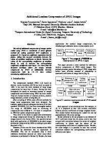
Figure 1. The schema of the proposed characteristic vector based approach Received on: 11.12.2011 Accepted on: 20.02.2012

1400


used for CCITT standard facsimile images [10]. Finally, a lossless compression method which uses chain codes was proposed in [13]. As seen above, most previous works in literature directly compress binary image data without taking care of the characteristic vector information of objects in them. However, analysis of the characteristic vectors of objects can provide efficiency for the compression algorithms. These vectors have very important information about geometrical features of objects. When determining characteristic vector information of binary image data having especially high size, the original image data can be presented in a very smaller size. Therefore, compressing only characteristic vectors instead of whole image data can provide a very high performance aspect of execution time and compression rate for especially artificial images such as technical drawings, icons or comics. In this article, we propose a novel lossless binary image compression scheme. The proposed scheme consists of two major steps: (i) firstly, encoding image data to only characteristic vector information of objects in image by using a new edge tracing method which aims to obtain simultaneously faultless edge points and geometrical shape information of objects by scanning image matrix only once. Therefore, both characteristic vector information of image is obtained and image data which have especially high size and artificial can be encoded to a very small size. (ii) compressing the encoded data using well-known other image compression algorithms such as Huffman, RunLength or Lempel-Ziv-Welch (LZW). In additional, the proposed scheme can reconstruct lossless copy of original image data from compressed data.

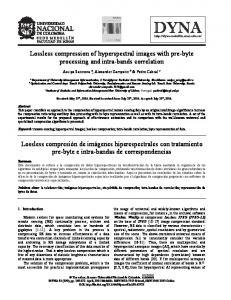
that more time can be given for other processes such as classification, compression or transmission that can be used after the recognition process. It consists of a main procedure and a subfunction. The main procedure determines the starting points of inner and outer edge lines of each independent object in image. The sub-function takes a starting point from the main procedure and it starts to investigate other edge points on edge line. While strolling on any edge line, the sub-function also obtains its geometrical information. In section (2.1.1) and (2.1.2) contains sequentially sufficient information about the modified starting point detection and edge tracing algorithms. 3.2. The detection algorithm of starting points The starting point detection algorithm determines only starting points of inner and outer edge lines of each independent object in binary image. According to the starting point detection algorithm, any independent object has an outer starting point. This point is the starting point of outer edge line of object. In addition, any independent object has inner starting points as its hole number as. These points are starting points of inner edge lines of objects. The flow diagram of the starting point detection algorithm is represented in Figure 2. The algorithm provides to reach all objects and holes in image. The vector variable used in the algorithm is

3. Proposed Method The proposed characteristic vector based approach is showed in Figure 1. All stages related to encoding, compressing, decompressing and reconstructing of binary image data are mentioned widely at following. 3.1. Encoding image data A modified version of the binary object recognition method in [11, 12] is used for encoding of whole image data to characteristic vectors. It can obtain rapidly all of the inner and outer contour lines of all objects in a binary image. The method consists of a new detection algorithm of starting point and an edge detection algorithm. It aims to obtain simultaneously faultless edge points and geometrical shape information of objects by scanning image matrix only once. Therefore, the object recognition process in binary images can be carried out very quickly. It means

Figure 2. Flow diagram of the starting point detection algorithm


1401

necessary for the edge tracing algorithm. 3.3. Edge tracing algorithm The edge tracing algorithm takes a point from the starting point detection algorithm. This point is the starting point of any inner or outer edge line. Starting from this point, the edge tracing algorithm determines other edge points on the edge line. During this tracing process, edge direction changes are saved and encoded by using the direction vectors in Figure 3. Hence, it is hindered to control all points of objects to obtain their edge points and geometrical information. Controlling less point means that the comparison number of the algorithm is decreases. Therefore, the algorithm operates in desired speed and performance. In Figure 4 is showed the flow diagram of the edge tracing algorithm. As is seen in the flow diagram, the edge tracing algorithm takes starting points and the starting vector value from the starting point detection algorithm.

Figure 4. Flow diagram the edge tracing algorithm

are taken into consideration in the controlling process. After the controlling process, the angle between the found point and the current point is expressed in Equation (1). Using this angle in Equation (2), new coordinate values of the found point are computed. Figure 3. Direction vectors used by edge tracing algorithm. Vector number takes 3, 2, 1, 0 in a, b, c, d.

Direction vectors are used to hold edge points of objects that have four main directions (left, right, top and bottom). Direction vectors give information about which direction we control to move to the subsequent edge point from the current edge point. Numbers on these vectors express the priority of the directions we should move. There is an angle of 900 among each vector. The edge tracing algorithm needs new direction number and vector number using former direction number and vector number to move to subsequent edge point from the current edge point. The new direction number is determined by controlling points at 8-neighboor of the current edge point. Direction numbers on the current vector

sa su

45* Direction 2 * Vector 2 * 180 sx round sin sy round cos

(1) (2)

When coming a new point in the edge tracing algorithm, it is also necessary to compute the new vector number for the following controlling process. The new vector number depends on the new direction number found. The new direction vector number is calculated by using the expression in Equation (3). The edge tracing algorithm can go ahead on edge lines on objects by renewing direction and vector values as mentioned above. The algorithm ends when it encounter to the starting point. Therefore, all inner and outer edge lines of objects can be determined by controlling only edge points of objects. (3)

1402

Field


(a) Field Description Width of the original image Height of the original image Characteristic vector information of edge points ( number of edge point ) Starting points of edge lines ( equals the total independent object and hole, it includes and points of each point) Filling Points ( equals the number of filled object, it and coordinate points of each point)

Size 2 Bytes 2 Bytes equals the number of coordinate includes

Variable*3 Bits Variable*3 Bytes

Variable*2 Bytes

(b) Field details Figure 5. (a)Encoded data format (b) Detail information of (a)

After completing the edge tracing algorithm, the encoded data format of original binary image shown in Figure 5 is obtained. The encoded data format consists of the dimensions of the original image (Size_Height and Size_Weight), characteristic vector information ( C ), starting points of edge lines ( D ), and filling points ( E ). The field C includes direction changes of edge points. Direction values in the field C are determined by using the direction vector in Figure 3. The field D includes starting points of inner and outer edge lines of each independent object in image. Each record in the field D includes information about one edge line. The field E includes first point of each filled object. Figure 6 presents an example binary image and result of the edge tracing algorithm for the image. Values x, y in the fields D and E are coordinate values of each point determined. The value pn in the field D shows the length of each edge line. 3.2. Compressing The field C obtained after the encoding process has a dataset with large size and its each

(a)

value is between 0 and 7 as is shown in Figure 8. Therefore, the array is very suitable to compress by using other compression techniques. In this article, we use Huffman and Lempel-Ziv-Welch (LZW) compression techniques which are known as lossless binary image compressing algorithms. The encoded array compressed by using these techniques will have been a quite small size. 3.3. Decompressing The decompressing process provides again obtaining of the encoded data. For this stage, one of the well known decompressing algorithms of Huffman or LZW can be used. 3.4. Decoding of The Encoded Data For the decoding process, first of all, a white image by using the dimensions of the original image which are Size_Height and Size_Weight is first drawn. Each record which consists of x, y and pn in the array D is sequentially read. Edge lines of objects are started to draw at x, y coordinate points of each record read. Length of each independent edge equals pn value of record read. Direction information of each

(b)

Figure 6. (a) Original binary image (b) Data of the original image and the encoded image.


edge line is available in the field C . Edge lines are reconstructed by using this information together with the direction vectors in Figure 3. After obtaining edge points of original image, interior parts of some objects determined prior are filled using the points of the field E . Therefore, obtaining image is exact copy of original image.

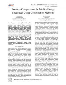
4. Experiments and Discussitions We compare the comparison result produced by Run-Length which is one of lossless binary image algorithms with our method. Run-Length algorithm was especially selected among traditional algorithms. Particularly for images of technical drawings, icons or comics, it is a very efficient algorithm. However, for CCITT standard facsimile images, it is not better than other algorithms such as Huffman and LZW. Comparisons are made aspects of compression ratio and execution time. Figure 8 shows twenty binary images which have different dimensions and objects with concave or convex geometrical shape. Table 1 shows the comparison of compression ratios for the selected images. Images between image1 and image9 have smaller size than images between image10 and image19. Analyzing carefully the obtained results from images between image1 and image9, it is shown clearly that Run-Length obtains better results than proposed methods for images such as image1, image3 and image4 which have flat objects. For other images between image1 and image9, its values of compression ratios

1403

approximate to values of proposed methods, but can not reach. Compression ratios of the proposed method used together with Huffman or LZW for images between image10 and image19 which have high dimensions are very good. Table 2 shows execution times of the proposed method for processes of encoding and comparison processes and Run-Length obtained on a Pentium III 1300 MHz personal computer with 768 MB RAM. It is shown clearly that the proposed method operates very fast because of compressing only edge lines.

5. Conclusions A novel lossless binary image compression scheme based on compressing only characteristic vector information of objects in images is presented. Unlike the existing approaches, our method encodes information of edge lines obtained using the modified edge tracing method in [11] instead of directly encoding whole image data. The encoded data is then compressed by using well-known other lossless image compression algorithms such as Huffman and LZW. We believe that the proposed method will able to provide a different point of view for traditional lossless binary image compression algorithms. Finally, we have shown in the experiments that the proposed method was able to compress at least %10 better than other traditional techniques. In addition to this advantage, execution times of the proposed method are less. Focusing on gray level images without noise, we will investigate to applicable of the proposed

Figure 8. Binary test images having objects with concave and convex geometrical shape.

1404


method. Table 1. Comparison of compression ratios for binary images. Image Name Image1 Image2 Image3 Image4 Image5 Image6 Image7 Image8 Image9 Image10 Image11 Image12 Image13 Image14 Image15 Image16 Image17 Image18 Image19

Black Point Num. Size 6227 100x100 4714 100x100 4348 100x100 4772 100x100 4332 100x100 4427 100x100 15731 256x256 19088 256x256 13725 256x256 49730 512x512 80255 512x512 88062 512x512 161318 512x512 65111 512x512 151599 512x512 74991 512x512 147364 512x512 68483 512x512 87759 512x512

Run-Length 76,733 31,700 42,600 43,867 34,667 23,033 70,744 5,390 14,053 74,473 80,748 69,716 70,439 76,504 82,146 70,928 81,349 63,223 74,569

Proposed Method with LZW 56,300 30,700 24,800 10,167 8,600 13,133 74,609 2,227 5,010 88,266 92,413 87,300 86,483 89,072 92,026 87,012 89,488 77,339 89,137

Proposed Method with Huffman 61,800 63,633 39,300 29,167 38,367 51,333 84,238 16,133 20,410 88,931 92,565 85,500 85,944 86,969 88,013 87,774 87,883 78,905 87,979

Table 2. Execution timings for compression of binary images in seconds. Image Name Image1 Image2 Image3 Image4 Image5 Image6 Image7 Image8 Image9 Image10 Image11 Image12 Image13 Image14 Image15 Image16 Image17 Image18 Image19

Run-Length 0,120 0,231 0,120 0,121 0,180 0,250 2,234 1,011 1,142 5,518 5,377 5,368 3,715 3,685 4,075 5,268 3,104 5,328 4,987

Encoding time 0,080 0,050 0,060 0,050 0,070 0,060 0,070 0,320 0,340 0,841 0,800 0,874 0,781 0,792 0,781 0,801 0,781 0,830 0,791

Proposed Method Comparison time with Comparison time Huffman with LZW 0,050 0,120 0,030 0,140 0,050 0,180 0,050 0,220 0,050 0,231 0,040 0,180 0,091 0,580 0,300 5,448 0,231 4,476 0,191 2,914 0,140 1,593 0,301 3,825 0,270 4,617 0,281 3,385 0,240 2,965 0,210 3,425 0,230 2,564 0,350 7,992 0,240 3,245


1405

6. References [1] Russ, J.C.: ‘The Image Processing Handbook’, North Carolina State University, pp.35-41, 2002. [2] Pitas, I.: ‘Digital Image Processing Algorithms and Applications’, United States of America, pp.242244, 2000. [3] Nelson M, Gailly JL. “Data Compression Book”, Second edition. New York: M&T Books, 1996. [4] Shi, Yun Q., and Sun, H., “Image and video compression for multimedia engineering”, ISBN 08493-3491-8, Chapter 6, pp.20-23, 2000. [5] Abdat, M., and Bellanger, M.G., “Combining Gray coding and JBIG for lossless image compression,” Proc. ICIP-94, vol.3 pp.851-855, 1999. [6] Culik, K. and Valenta, V., “Finite automata based compression of bi-level images,” Proc. Data Compression, pp.280-289, 1996. [7] Phimoltares, S., Chamnongthai, K., and Lursinsap, C., “Hybrid Binary Image Compression”, Fifth International Symposium on Signal Processing and its Applications, ISSPA ’99, Brisbane, Australia, 1999. [8] Tompkins, D., and Kossentini, F., “A Fast Segmentation Algorithm for Bi-Level Image Compression using JBIG2”, 0-7803-5467-2/99, IEEE, 1999. [9] Bogdan J. F., “Lossless binary image compression using logic functions and spectra”, Computers and Electrical Engineering 30, pp.17–43, 2004. [10] CCITT Standard Fax Images at http://www.cs.waikato.ac.nz/~singlis/ccitt.html. [11] Turkoglu, I. and Arslan, A., “An Edge Tracing Method Developed For Object Recognition”, The 7-th International Conference in Central Europe on Computer Graphics, pp. 9-12, Plzen, Slovakia (1999) [12] Talu, M.F., Tatar, Y., “A new edge tracing method developed for object recognition”, TAINN 2003, Çanakkale, Haziran 2003. [13] Akimov, A., Kolesnikov, A. and Franti, P., "Lossless compression of map contours by context tree modeling of chain codes", Pattern Recognition, 40 (3), 944-952, March 2007.

M. Fatih TALU received the B.Sc. degrees in Computer Engineering and M.Sc. and Ph.D. degrees in ElectricalElectronics Engineering of the Firat University, Elazig, Turkey, in 2003, 2005, and 2010. He is currently an Assistant Professor in Computer Engineering Department of Inonu University. His research interests include object tracking, machine learning and feature extraction methods.

Ibrahim TURKOGLU was born in Elazig, Turkey, 1973. He received the B.S., M.S. and Ph.D.degrees in ElectricalElectronics Engineering from Firat University, Turkey in 1994, 1996 and 2002 respectively. He is working as an assistant professor in Electronics and Computer Science at Firat University. His research interests include artificial intelligent, pattern recognition, intelligent modeling, radar systems and biomedical signal processing.