Hybrid Modeling and Simulation of Biomolecular Networks - CiteSeerX

Hybrid Modeling and Simulation of Biomolecular Networks Rajeev Alur, Calin Belta, Franjo Ivancic, Vijay Kumar, Max Mintz, George Pappas, Harvey Rubin, and Jonathan Schug University of Pennsylvania

Abstract. In a biological cell, cellular functions and the genetic regulatory apparatus are implemented and controlled by a network of chemical reactions in which regulatory proteins can control genes that produce other regulators, which in turn control other genes. Further, the feedback pathways appear to incorporate switches that result in changes in the dynamic behavior of the cell. This paper describes a hybrid systems approach to modeling the intra-cellular network using continuous dierential equations to model the feedback mechanisms and mode-switching to describe the changes in the underlying dynamics. We use two case studies to illustrate a modular approach to modeling such networks and describe the architectural and behavioral hierarchy in the underlying models. We describe these models using Charon [2], a language that allows formal description of hybrid systems. We provide preliminary simulation results that demonstrate how our approach can help biologists in their analysis of noisy genetic circuits. Finally we describe our agenda for future work that includes the development of models and simulation for stochastic hybrid systems. We believe that an understanding of the redundant design for robust regulation of noisy biological processes may help engineers in designing, organizing and programming distributed embedded systems.

1 Introduction In order to survive, organisms continuously monitor their surroundings and, if necessary, adjust trac through single or complex combinations of genetic and metabolic networks to respond to alterations in local conditions. Local conditions include both the physical environment, for example, temperature (the heat and cold shock response), nutrient and energy source concentrations (the stringent response), light (circadian rhythms), cell density (quorum sensing response) as well as the molecular environment of individual regulatory components. Examples of the latter include intracellular concentrations of transcription factors and allosteric eectors. The availability of complete genomic information for a wide variety of organisms and the consequent attention on proteomics has dramatically increased the number of systems and components of systems that are involved in these sensing and responding activities [4, 10]. Understanding how these biological systems are integrated and regulated and how the regulation may be in uenced, possibly for therapeutic purposes, remains a signi cant challenge. In this paper we model and simulate examples of genetic and metabolic networks using a hybrid systems approach that combines concepts and tools from control theory and computer science. First we analyze a previously published plasmid-based genetic network that was designed and synthesized using three repressor transcription factors where one repressor negatively regulates the production of a subsequent repressor [7]. Then we model a biologically important genetic network that controls the quorum sensing response, an adaptive response of certain gram negative bacteria to local population density [13, 17]. The quorum sensing response controls the luminescent behavior in certain strains of Vibrio which has been linked to the normal development of the bacterial host [18] as well as to medically important phenomena such as bio lm formation by Pseudomonas aerugenosa, an organism that can cause overwhelming pneumonia and septic shock [11, 20].

2 Modeling The genetic circuits and biomolecular networks considered here and elsewhere are remarkably similar to hybrid systems encountered in engineering, for example embedded systems. In particular, it is worth noting the following three key features:

Concurrency and communication. At the intra-cellular level, proteins and/or mRNAs are agents

communicating with each other and in uencing each other's behavior. At the inter-cellular level, cells can be viewed as networked agents interacting with each other via dierent communication mechanisms. Discrete and continuous behaviors. At the lowest level, the evolution of entities such as proteins can be described by dierential equations. Discreteness arises in two ways. First, a certain activity may be triggered only when the concentration of enabling quantities is above the desired threshold. This leads to discrete switching between active and dormant states. Second, dierent models may be appropriate at dierent levels of concentration. Stochastic behavior. Evolution of entities is not deterministic, and is better captured by stochastic models that allow for uncertainty and noise. These characteristics are typical of high-level models of embedded software such as autonomous communicating mobile robots. For describing such systems, we have developed the language Charon [2] which incorporates ideas from concurrency theory (languages such as CSP [12]), object-oriented software design notations (such as Statecharts [9] and UML [3]), and formal models for hybrid systems (such as hybrid automata [1] and hybrid I/O automata [15]). The key features of Charon are:

Architectural hierarchy. The building block for describing the system architecture is an agent that

communicates with its environment via shared variables. The language supports the operations of composition of agents to model concurrency, hiding of variables to restrict sharing of information, and instantiation of agents to support reuse. Behavior hierarchy. The building block for describing ow of control inside an atomic agent is a mode. A mode is basically a hierarchical state machine, that is, a mode can have submodes and transitions connecting them. Variables can be declared locally inside any mode with standard scoping rules for visibility. Modes can be connected to each other only via well-de ned entry and exit points. We allow sharing of modes so that the same mode de nition can be instantiated in multiple contexts. Finally, to support exceptions , the language allows group transitions from default exit points that are applicable to all enclosing modes. Discrete updates. Discrete updates are speci ed by guarded actions labeling transitions connecting the modes. Actions can have calls to externally de ned Java functions which can be used to write complex data manipulations. It also allows us to mimick stochastic aspects through randomization. Continuous updates. Some of the variables in Charon can be declared analog, and they ow continuously during continuous updates that model passage of time. The evolution of analog variables can be constrained in three ways: dierential constraints (e.g. by equations such as x_ = f (x; u)), algebraic constraints (e.g. by equations such as y = g(x; u)), and invariants (e.g. jx ? yj  ") which limit the allowed durations of ows. Such constraints can be declared at dierent levels of the mode hierarchy. Modular features of Charon allow succinct and structured description of complex systems. Similar features are supported by the languages Shift [6] and Stateflow (see www.mathworks.com). In Charon, modularity is not only apparent in syntax, but we are developing analysis tools (such as simulation) that exploit this modularity. Furthermore, Charon has formal foundations supporting compositional re nement calculus which allows relating dierent models of the system in mathematically precise manner.

3 Modeling Biomolecular Networks in Charon As noted in [5], most biomolecular systems of interest involve many interactions connected through positive and negative feedback loops, so that an intuitive understanding of their dynamics is hard to obtain. In this section we will describe the modeling of a speci c biomolecular network. We will model a repressilator system described in [7]. First we provide some biological background information and describe the protein network used in [7], and then describe the models of the protein network, including examples of Charon models. Due to the lack of correct parameter values, we do not provide simulation results in this section.

3.1 A Protein Repressilator System

In the synthetic oscillatory network described in [7], networks of interacting biomolecules carry out many essential functions in living cells. But the design principles of the functioning of such networks still remain poorly understood { even in relatively simple systems [14]. The authors proposed the design and construction of a synthetic protein network implementing a particular function. Their idea is that such a \rational network design" may lead to the engineering of new cellular behaviors and to improved understanding of naturally occuring networks. The repressilator system described in [7] contains three proteins, namely lacI, tetR, and cI. The protein lacI represses the protein tetR, tetR represses cI, whereas cI represses lacI, thus completing a feedback system called a repressilator system. The dynamics of the network depend on the transcription rates, translation rates, and decay rates of proteins and messenger RNAs. Depending on the values of the dierent parameters in the model, the system might converge to a stable limit cycle or become unstable.

3.2 The Models of the Protein Repressilator System

It is well known in mechanics and thermodynamics that there are two dierent approaches to modeling such systems. At reasonably high molecular concentrations, one can adopt continuum models which lend themselves to deterministic models involving ordinary and partial dierential equations. At lower concentrations, the discrete molecular interactions become important and deterministic models are dicult to obtain [8].

The Deterministic, Continuous Approximation. We will consider the three repressor protein concentrations pi ; i 2 P = flacI; tetR; cIg and their corresponding mRNA concentrations mi ; i 2 P as con-

tinuous dynamic variables. The system kinetics are determined by the following six coupled rst-order dierential equations.

dmi = ?m +  +  0 i 1 + pn dt j dpi = ? (p ? m ) i i dt   i = lacI, tetR, cI j = cI, lacI, tetR

The equations use various constants. The "leakiness of the promoter"  is the number of protein copies per cell produced from a given promoter type during continuous growth in the presence of saturating repressor amounts. During the absence of the repressor, we have  + 0 number of protein copies per cell. The ratio of the protein decay rate to the mRNA decay rate is denoted by , while n stands for the so called Hill coecient.

The Stochastic, Discrete Approximation. The continuous analysis neglects the discrete nature of molecular components and the stochastic character of their interaction [7]. Following [7], we adopt the stochastic approximation as described by Gillespie in [8]. 3.3 Modeling the Repressilator System in Charon

In this section we will present the repressilator system models as described in [7] using the Charon language. We will present many of the advantages that the Charon language has to oer for modeling such biomolecular models. Our model will de ne a general protein model as an agent in Charon. We will instantiate this agent model to obtain the three proteins lacI, tetR, and cI. The approximation models will be implemented inside the modes of the protein agent. To present another feature of our language, we will also describe a combination of the discrete and the continuous model into one modeling system.

The Protein Agent in the Continuous Approximation. In this section we will describe a Charon model of a general protein agent. We have a continuous input variable which represents the repressor protein concentration pR . This means, that the environment of this protein agent supplies the value of this variable, and it cannot be changed by the protein agent. The protein agent has a continuous private variable representing the messenger RNA concentration. Private variables cannot be seen outside the agent and can be updated internally for internal use only. The output of the protein agent is a continuous variable representing the protein concentration. Output variables are updated by the agent, and can be used as input variables in the environment. The general protein agent has parameters 0 ; ; ; n; p0 ; and m0 . By instantiating these parameters with values, we can obtain instantiated protein agents representing a speci c protein. The parameters p0 and m0 will be used for initialization purposes and stand for the initial protein concentration and the initial messenger RNA concentration respectively. The following represents the corresponding Charon code. agent contProtein ( real p0 , m0 , alpha0 , alpha , beta , n ) { write analog real p = p0 ; //protein concentration read analog real pR ; //repressor protein concentration private analog real m = m0 ; //messenger RNA concentration /* Notice the way we initialized the protein concentration p and the messenger RNA concentration m using p0 and m0. */ mode cont = continuous ( alpha0 , alpha , beta , n ) ; }

protein agent local m parameters: p0,m0,alpha0,alpha,beta,n read pR

p=p0 m=m0

continuous mode

write p

d(m)=-m+alpha/(1+pR^n)+alpha0 d(p)=-beta*(p-m)

Fig. 1. A general protein agent for the continuous approximation model We still need to de ne the behavior of the agent. The behavior is described by the modes of the agent. The behavior of the general protein agent is de ned in cont, which is an instaniation of a general continuous mode de nition that is de ned by the following code. A graphical version of the general protein model can be found in Figure 1. mode continuous ( real alpha0 , alpha , beta , n ) { write analog real p ; //protein concentration read analog real pR ; //repressor protein concentration private analog real m ; //messenger RNA concentration diff mRNA { /* Here we define the differential equation that computes

the messenger RNA concentration m. We use the repressor protein concentration pR. */ d(m) = -m + alpha / (1+pR^n) + alpha0 } diff proteinConcentration { /* Here we define the differential equation that computes the protein concentration p. We use the messenger RNA concentration m. */ d(p) = -beta * (p-m) } }

RepressilatorSystem lacI

p1

tetR

p2

cI

p3

Fig. 2. Composed repressilator system using the instantiated general protein agent

Instantiation and Parallelism. We de ned a general protein agent in the previous section. We have to instantiate this general agent model to get the three proteins used in the system. We also want the three proteins lacI, tetR, and cI to run in parallel and to in uence each other. We have to provide values for the parameters of the protein agent, which we do not bother to show in our code here. Notice the use of renaming of variables to couple the three instantiated protein agents to in uence each other. A graphical version of the composed system is illustrated in Figure 2. The following represents the corresponding Charon code using some values for the parameters of the protein agent. agent RepressilatorSystem () { private analog real p1 , p2 , p3 ; agent lacI = contProtein ( ... ) [ p , pR := p1 , p3 ] ; agent tetR = contProtein ( ... ) [ p , pR := p2 , p1 ] ; agent cI = contProtein ( ... ) [ p , pR := p3 , p2 ] ; }

The Protein Agent in the Discrete Approximation. In this section we will present a possible model

for a discrete approximation of a protein agent. As we did it for the continous case, we will again de ne a general protein agent, that can be instantiated to build a system of proteins. Our model will work as follows. We will have an integer variable n that will keep track of the number of protein molecules which will be the output of the agent. The input to the agent will be the number of repressor protein molecules nR . Depending on various parameters, we want to increase or decrease the number of protein molecules by one at a time. The basic idea is to use stochastic simulation as described in [8]. The parameters that in uence the stochastic simulation are binding and unbinding of proteins on two-sided promoters,

the protein and mRNA decay rates, and translation. The corresponding Charon code is shown in the Appendix.

protein agent local m

discrete mode

read pR

write p continuous mode

discreteTiming

Fig. 3. A general protein agent for the combined framework using continuous and discrete approximation model

Combining the two Models into one Framework. The two dierent models for the repressilator system can be combined into one framework. The basic idea is to use the deterministic continuous model whenever the concentration of the protein is high enough, whereas we would switch to the discrete, stochastic model if the concentration would fall below a certain threshold value. Figure 3 gives an intuitive graphical representation of the protein agent with both the continuous and discrete approximation.

4 Hybrid Systems Models for Quorum Sensing A good illustration of multicellular behavior in prokaryotes is cell-density-dependent gene expression. In this process, a single cell is able to sense when a quorum of bacteria, a minimum population unit, is achieved. Under these conditions, certain behavior is eciently performed by the quorum, such as bioluminescence, which is the best known model for understanding the mechanism of cell-density-dependent gene expression. In this section, we will describe a hybrid system model that captured the changes in dynamics of the biochemical reactions observed in the literature [13, 16, 17].

4.1 Description of phenomena Vibrio scheri is a marine bacterium that can be found both as free-living organism and as a symbiont of some marine sh and squid. As a free-living organism, V. sheri exists at low densities (less than 500 cells per ml of seawater) and appears to be non-luminescent. As a symbiont, the bacteria live at high densities and are, usually, luminescent. In a liquid culture, the bacteria's level of luminescence is low until the culture reaches mid to late exponential phase. A dramatic increase in luminescence is observed at that time due to the transcriptional activation of the lux genes. Once the bacteria reach stationary phase, the level of luminescence decreases. The lux regulon [17] contains two operons, OL and OR (see Figure 4). The left operon OL contains the luxR gene encoding the protein LuxR, a transcriptional activator of the system. The right operon OR contains seven genes luxICDABEG. Protein LuxI, the product of the luxI gene is required for endogenous production of autoinducer, a small molecule capable of diusing in and out of the cell membrane. Genes luxA and luxB encode two subunits of luciferase. The trio luxC, luxD, and luxE code for the subunits of a protein complex which provides an aldehyde substrate for luciferase. The function of luxG is unknown. The autoinducer Ai binds to protein LuxR to form a complex Co. The two operons are separated by a regulatory region that contains a binding site for the cyclic AMP receptor protein CRP and a binding site for the complex Co.

CRP

Co binding site

luxICDABEG

luxR CRP binding site

Co

luxA luxR

+

Ai

Substrate

+

luxI

luxB

luciferase

Fig. 4. A portion of DNA emphasizing luxR and luxICDABEG genes and the binding sites for luxR complex and CRP

4.2 Transcription control of operons OL and OR

The transcription of luxR is regulated by both CRP and Co. We can distinguish between the following three dierent cases: { Case OL-1 In the absence of the autoinducer, CRP activates OL expression by initiating two RNA transcripts. { Case OL-2 At low autoinducer concentrations, luxR transcription is stimulated by increasing CRPdependent transcription and by Co-dependent transcription from another transcriptional start site. { Case OL-3 At high autoinducer concentrations, luxR transcription is repressed through a second, weaker Co binding site located in luxD. Likewise, transcription of OR is regulated by both CRP and Co. We distinguish two dierent cases: { Case OR -1 In the absence of autoinducer, CRP represses OR transcription. { Case OR -2 In the presence of autoinducer, Co activates transcription of OR. These cases will be interpreted as modes as seen later in the paper.

4.3 Development of a mathematical model

In this section, we develop a mathematical model for the luminescence phenomenon in one bacterium of V. scheri, describing the concentrations of the relevant mRNA's, proteins, and small molecules. As described in Section 4.2 the mechanism of transcription activation of both operons is highly dependent on the concentration of autoinducer, so the time evolution of the system cannot be described by one set of continuous dierential equations.1 Combining cases for OL and OR given in the previous section, yields three modes, which we call OFF, POS and NEG. The transitions between modes are governed by the level of internal autoinducer which we represent by [Ai]. Mode OFF corresponds to very low or zero concentration of autoinducer ([Ai]  [Ai]? ) within the bacterium and no luminescence is observed. The system is in mode POS when the concentration of internal autoinducer is low ([Ai]?  [Ai]  [Ai]+ ). This mode corresponds to positive growth and increasing concentration of autoinducer. Luminescence is observed, as are higher concentrations of proteins LuxA, LuxB, LuxC, LuxD, and LuxE. The transition to mode NEG (negative growth) occurs at high levels of autoinducer ([Ai] > [Ai]+ ). We use the following rate equation to describe the concentration for any molecular species (mRNA, protein, protein complex, or small molecule) [19]: d[x] = synthesis ? decay  transformation  transport (1) dt 1

In [13], the dierential equations for the low autoinducer concentration are described. The model presented here describes a wider range of operating conditions.

The synthesis term represents transcription for mRNA and translation for proteins. The decay term represents a rst order degradation process. The transformation term describes reactions such as cleavage or ligand-binding that do not destroy the protein, but do remove its ability to participate in speci c reactions. Finally, molecular species may participate in transport processes, like passive diusion or active transport through a membrane. The biomolecular system can be described in a nine dimensional state space. The nine variables, x1 ; x2 ; : : : ; x9 , describe the concentrations of dierent molecules as follows:

x1 = mRNA transcribed from OL , x2 = mRNA transcribed from OR , x3 = protein LuxR, x4 = protein LuxI, x5 = protein LuxA, x6 = protein LuxB, x7 = autoinducer inside the bacterium Ai, x8 = LuxR:Ai complex Co, x9 = autoinducer outside the bacterium Aiex ,

where Ai is the dimensionless version of [Ai].

For simplicity, we have assumed that the concentrations of CRP and of the substrate necessary for endogenous production of Ai are constant. Further, we have neglected the decay rates for chemical compounds. Finally, we assume that the concentrations of LuxC, LuxD, and LuxE are similar to those of LuxA and LuxB. The (continuous) dierential equations for each mode are of the form x_ = f i (x) where x = [x1 ; x2 ; : : : ; x9 ]T 2 9 , f i = [f1i ; f2i ; : : : ; f9i ], and i 2 fOFF; POS; NEGg. The components of the vector elds are explicitly given by:  1 OFF f1 = 1 2 c ? x 1 IR

f1POS f1NEG f2OFF f2POS = f2NEG f3i f4i f5i f6i f7i f8i f9i

  81  x 1 8 = 4 3c + 81 + x81 ? 4x1 = ?1 x1 = ?2 x2

81

82

8



8 = 2 82x+  ? x2 82 x882 = 3 (x1 ? x3 ) ? r37;Ai x3 x7 = 4 (x2 ? x4 ) ? r4 x4 = 5 (x2 ? x5 ) = 6 (x2 ? x6 ) = ?7 x7 + r4 x4 ? rmem (x7 ? x9 ) ? r37;R x3 x7 = ?8 x8 + r37;Ai x3 x7 = ?7 x9 + rmem (x7 ? x9 ) + u where, in the last seven equations fji is independent of the mode. All the quantities in the above model are non-dimensional. i = T0 =Hi where T0 is the characteristic time constant of the system and Hi is the half-life (inverse of the decay rate) of molecule xi . ij is a cooperativity coecient while ij describes the potency of the regulation of the transcription of mRNA j by protein i. r denotes transformation and transfer rates. For example rmem is the transfer rate of autoinducer through the membrane of the cell while r37;R and r37;Ai are transformation rates obtained by non-dimensionalizing the binding rate of the reaction between Ai and LuxR in two dierent ways. c is dependent on the concentration of CRP and its anity to the corresponding binding site, and, as stated earlier, is assumed to be constant. Finally, u emulates an external source of Ai and is used to simulate the sensitivity of the bacterium to changes of autoinducer concentration in the exterior.

We regard u as an input to our system. Since proteins LuxA and LuxB are subunits of luciferase, which produces luminescence, it is reasonable to assume that the level of luminescence is proportional to the product of the concentrations of LuxA and LuxB, which we choose to be the output of the system.

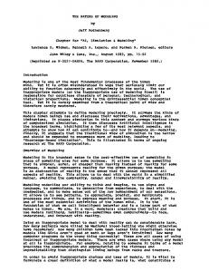
4.4 Charon implementation The behavioral hierarchy in Charon (see Figure 5) is characterized by three dierent behaviors which

are represented by three dierent modes, namely OFF, POS, and NEG. Many of the dierential equations governing the dynamics of the system are shared between the modes. We will introduce the notion of mode hierarchy to extract the shared constraints. Through the notion of submodes and scoping, we can simplify the description of the respective modes OFF, POS, and NEG. agent vibrio_fischeri

x& j = f ji ( x ), i ∈ { OFF , POS ,ON },

j = 3 ,...,9

mode POS-NEG

mode OFF

x&1 ,2 = f 1OFF ,2 ( x )

mode POS

Ai > Ai− Ai < Ai−

x&1 = f 1POS ( x )

x&2 = f 2i ( x ), i ∈ { POS , NEG }

Ai > Ai+ Ai < Ai+

mode NEG

x&1 = f1NEG ( x )

Fig. 5. Charon structure of the system

4.5 Simulation results

Figure 6 illustrates the response (i.e., luminescence) of the bacterium to a perturbation in the concentration of external autoinducer that takes the form of a rectangular pulse. The magnitude of the step has been chosen to make the system go through all three modes. The results con rm the experimental observations [17]: luminescence increases during mode POS and decreases in mode NEG; there is no luminescence in mode OFF. The switch history and the time evolution of the concentrations of the signi cant molecules in the system are also shown. In mode OFF, all molecules decay to zero, except for mRNA OL and the corresponding protein R, as expected. For a short time, in mode POS, all the concentrations increase until the internal autoinducer reaches a high concentration, when the system is switched to mode NEG. In this last mode, everything decays to zero, except for internal autoinducer which can reach a stable non-zero value dependent on the size of the step of external autoinducer.

5 Conclusions In this paper we have shown that biological cellular networks can be naturally modeled as hybrid systems. In particular, the protein repressilator system switches between a continuous deterministic model at high concentrations, and a timed, discrete, stochastic model at low concentrations. Similarly, the luminescence control of Vibrio scheri is naturally modeled as a multi-modal hybrid system, resulting in simulations that are in accordance with experimental observations. The hybrid nature of such protein networks can be very easily expressed and simulated in Charon, which may oer us better and a more global understanding of biological networks. The enormous complexity of large scale biological networks will present us with great challenges that we must face. Exploiting the structure of biological systems will be critical for scaling the applicability

(a)

(b)

1

NEG

0.5

POS

0

0

200

400

OFF

600

mRNA O L 1 O mRNA

(c) 0.08

(d)

R

R I

0.06 0.04

0.5

0.02 0

0

200

400

600

0

0

200

NEG

400

600

400

600

(e)

(b) 1 A B AI CO

POS

0.5

OFF

0

0

200

Fig. 6. Increase in external autoinducer produces luminescence: (a)input - external source of autoinducer; (b) switch hystory; (c) output (luminescence)- product of concentrations of proteins A and B ; (d) and (e) time evolution of concentrations; of the modeling, analysis, and simulation tools. It is therefore extremely encouraging that the two case studies presented in this paper exhibit the architectural paradigms of modern software engineering. We envision the link between hybrid systems technology, and biology to strengthen. The scalable nature of computational tools like Charon will enable the uni ed and improved modeling of biological cellular networks, leading to better understanding, as well as providing us with the opportunity to determine how local biological changes can aect global behavior. Conversely, a good understanding of the robustness of noisy biological networks will lead to new approaches to designing networked embedded systems. The case studies also highlight the need for developing a theory of stochastic hybrid systems, for instance, for modeling rate equations of biochemical reactions. Useful mathematical tools for analysis of such systems are rare, and developing adequate computational tools for understanding such models will be a challenging research area.

References 1. R. Alur, C. Courcoubetis, N. Halbwachs, T.A. Henzinger, P. Ho, X. Nicollin, A. Olivero, J. Sifakis, and S. Yovine. The algorithmic analysis of hybrid systems. Theoretical Computer Science, 138:3{34, 1995. 2. R. Alur, R. Grosu, Y. Hur, V. Kumar, and I. Lee. Modular speci cations of hybrid systems in charon. In Hybrid Systems: Computation and Control, Third International Workshop, volume LNCS 1790, pages 6{19, 2000. 3. G. Booch, I. Jacobson, and J. Rumbaugh. Uni ed Modeling Language User Guide. Addison Wesley, 1997. 4. R. Brent. Genomic biology. Cell, 100(1):169{183, January 2000. 5. H. de Jong, M. Page, C. Hernandez, H. Geiselmann, and S. Maza. Modeling and simulation of genetic regulatory networks. ERCIM News, 43, October 2000. 6. A. Deshpande, A. Gollu, and L. Semenzato. Shift programming language and run-time systems for dynamic networks of hybrid automata. Technical report, University of California at Berkeley, 1997. 7. M. Elowitz and S. Leibler. Asynthetic oscillatory network of transciptional regulators. Nature, 403:335{338, January 2000. 8. D.T. Gillespie. Exact stochastic simulation of coupled chemical reactions. J. Phys. Chem., 81:2340{2361, 1977. 9. D. Harel. Statecharts: A visual formalism for complex systems. Science of Computer Programming, 8:231{274, 1987. 10. L.H. Hartwell, J.J. Hop eld, S. Leibler, and A.W. Murray. From molecular to modular cell biology. Nature, 402((6761 Suppl)):C47{52, December 1999.

11. D.J. Hassett, J.F. Ma, J.G. Elkins, T.R. McDermott, U.A. Ochsner, S.E. West, C.T. Huand, J. Fredericks, S. Burnett, P.S. Stewart, G. McFeters, L. Passador, and B.H. Iglewski. Quorum sensing in pseudomonas aeruginosa controls expression of catalase and superoxide dismutase genes and mediates bio lm susceptibility to hydrogen peroxide. Mol Microbiol, 34(5):1082{1093, December 1999. 12. C.A.R. Hoare. Communicating Sequential Processes. Prentice-Hall, 1985. 13. S. James, P. Nilson, G. James, S. Kjellenberg, and T. Fagerstrom. .luminescence control in the marine bacterium vibrio scheri: An analysis of the dynamics of lux regulation. J Mol Biol, 296(4):1127{1137, March 2000. 14. D.E. Jr Koshland. The era of pathway quanti cation. Science, 280:852{853, 1998. 15. N. Lynch, R. Segala, F. Vaandrager, and H. Weinberg. Hybrid I/O automata. In Hybrid Systems III: Veri cation and Control, LNCS 1066, pages 496{510, 1996. 16. H. H. McAdams and A. Arkin. Simulation of prokaryotic genetic circuits. Annu. Rev. Biophys. Biomol. Struct., 27:199{224, 1998. 17. D.M. Sitnikov, J.B. Schineller, and T.O. Baldwin. Transcriptional regulation of bioluminesence genes from vibrio scheri. Mol Microbiol, 17(5):801{812, September 1995. 18. K.L. Visick, J. Foster, J. Doino, M. McFall-Ngai, and E.G. Ruby. Vibrio scheri lux genes play an important role in colonization and development of the host light organ. Bacteriol, 182(16):4578{4586, August 2000. 19. G. von Dassow, E. Meir, E. M. Munro, and G. M. Odell. The segment polarity network is a robust development module. Nature, 406:188{192, July 2000. 20. H. Yang, M. Matewish, I. Loubens, D.G. Storey, J.S. Lam, and S. Jin. miga, a quorum-responsive gene of pseudomonas aeruginosa, is highly expressed in the cystic brosis lung environment and modi es lowmolecular-mass lipopolysaccharide. Microbiology, 146((Pt 10)):2509{2519, October 2000.

Appendix: Charon Code of the Protein Agent in the Discrete Approximation mode discrete ( ... ) { read discrete int nR ; //number of repressor proteins write discrete int n ; //number of proteins private discrete int m ; //number of messenger RNA private analog real t ; //timer private discrete real tau ; //Gillespies' timing constant private discrete int choice ; //pick a reaction out of {1,2,3,4} mode timing = discreteTiming ( ... ) ; trans initT from default to timing do { t = 0 ; tau = f_1 ( ... ) ; choice = f_2 ( ... ) ; //also, initialize n and m with parameters } trans update when ( t do { n = t = when ( t do { n = t = when ( t do { m = t = when ( t do { m = t =

from timing to timing = tau && choice = 1 ) n + 1 ; 0 ; tau = f_1 ( ... ) = tau && choice = 2 ) n - 1 ; 0 ; tau = f_1 ( ... ) = tau && choice = 3 ) m + 1 ; 0 ; tau = f_1 ( ... ) = tau && choice = 4 ) m - 1 ; 0 ; tau = f_1 ( ... )

} mode discreteTiming ( ... )

; choice = f_2 ( ... ) ; }

; choice = f_2 ( ... ) ; }

; choice = f_2 ( ... ) ; }

; choice = f_2 ( ... ) ; }

{ readwrite analog real r , s , t , u ; readwrite discrete real dr , ds , dt , du ; read discrete int nR ; write discrete int n ; readwrite discrete int m ; diff time { d(r) = 1 ; d(s) = 1 ; d(t) = 1 ; d(u) = 1 ; } inv set { r