Hindawi Publishing Corporation Mathematical Problems in Engineering Volume 2016, Article ID 2030647, 14 pages http://dx.doi.org/10.1155/2016/2030647
Research Article Hybrid Models Based on Singular Values and Autoregressive Methods for Multistep Ahead Forecasting of Traffic Accidents Lida Barba1,2 and Nibaldo Rodríguez1 1
Escuela de Ingenier´ıa Inform´atica, Pontificia Universidad Cat´olica de Valpara´ıso, 2362807 Valpara´ıso, Chile Facultad de Ingenier´ıa, Universidad Nacional de Chimborazo, 060102 Riobamba, Ecuador
2
Correspondence should be addressed to Lida Barba;
[email protected] Received 29 December 2015; Accepted 5 May 2016 Academic Editor: Giovanni Falsone Copyright © 2016 L. Barba and N. Rodr´ıguez. This is an open access article distributed under the Creative Commons Attribution License, which permits unrestricted use, distribution, and reproduction in any medium, provided the original work is properly cited. The traffic accidents occurrence urges the intervention of researchers and society; the human losses and material damage could be abated with scientific studies focused on supporting prevention plans. In this paper prediction strategies based on singular values and autoregressive models are evaluated for multistep ahead traffic accidents forecasting. Three time series of injured people in traffic accidents collected in Santiago de Chile from 2000:1 to 2014:12 were used, which were previously classified by causes related to the behavior of drivers, passengers, or pedestrians and causes not related to the behavior as road deficiencies, mechanical failures, and undetermined causes. A simplified form of Singular Spectrum Analysis (SSA), combined with the autoregressive linear (AR) method, and a conventional Artificial Neural Network (ANN) are proposed. Additionally, equivalent models that combine Hankel Singular Value Decomposition (HSVD), AR, and ANN are evaluated. The comparative analysis shows that the hybrid models SSA-AR and SSA-ANN reach the highest accuracy with an average MAPE of 1.5% and 1.9%, respectively, from 1- to 14-step ahead prediction. However, it was discovered that HSVD-AR shows a higher accuracy in the farthest horizons, from 12- to 14-step ahead prediction, which reaches an average MAPE of 2.2%.
1. Introduction Traffic accidents with fatalities and severely injured people are a socioeconomic problem of focus. According to the WHO [1], the traffic accidents cost between 1% and 3% of the GDP of a country, regardless of invaluable emotional damage for the victims and their families. Several studies have been developed to explain the nature of the problem, most through classification; diverse methods have been used to detect the key factors that influence the incidents severity. Abell´an et al. (2013) used decision trees to extract some key patterns of severe accidents in Granada; the rules were defined in function of the variables related to atmospheric factors, driver characteristics, road conditions, or a factor combination [2]. Chang and Chien applied a method based on nonparametric classification and regression tree to establish the empirical relationship between injury severity and driver/vehicle characteristics in truck-involved accidents [3]. De O˜na et al. (2013) use Latent Class Clustering and Bayesian networks
to identify the variables involved in traffic accidents; the accident type and sight distance were detected in all the traffic accidents on rural highways in Granada [4]. Recently, Shiau et al. (2015) presented Fuzzy Robust Principal Component Analysis (FRPCA) combined with Backpropagation Neural Network (BPNN) to identify the relationships between the variables of road designs, rule-violation items, and accident types; the results showed an 85.89% classification accuracy [5]. Lin et al. (2015) used real time traffic accidents in a highway in Virginia; they found that the best model was based on Frequent Pattern and a Bayesian network; the model predicted 61.1% of accidents while having a false alarm rate of 38.16% [6]. The risk indicating variables of traffic accidents have been identified taking into consideration diverse factors; some factors are related to road design parameters [7, 8], environment conditions [9], traffic signs, or interactions among some factors [10]. The data provided by the Chilean Commission of Traffic Safety (CONASET) [11] shows a high and increasing rate of
2 fatalities and injuries in traffic accidents from 2000 to 2014. Santiago is the most populated Chilean region, whose time series of injured people is used in this analysis. The abundance of information and research about traffic accidents, severities, risks, and occurrence factors, among others, might appear somewhat unapproachable in terms of the prevention plans. In this case study, with categorical causes defined by CONASET and the ranking method, the potential causes of injuries in traffic accidents, which can be counteracted through campaigns directed to the change of attitude in drivers, passengers, and pedestrians toward road safety, have been identified. Two groups have been created based on the primary and secondary causes which are present in around 75% of injured people, and a third group was created with the remaining 25%. At first, nonstationary and nonlinear characteristics were found in the time series, turning the forecasting into a difficult task. Some researches exploit the potentialities of the SSA technique to extract components in a time series; SSA commonly has been used to extract trend, seasonality, and/or noise [12]; the extracted components are used to explain the complex behavior of some time series in diverse ambit, from nature [13, 14] to industrial process [15], or economic indicators [16]. On the other hand, the combination of SSA and autoregressive linear and nonlinear methods is a recent alternative which has demonstrated robustness and universal capacities in terms of short-term forecasting [17–19]. SSA combined with artificial intelligence techniques was used by Xiao et al. (2014) for monthly air transport demand forecasting [20]; a similar combination was made by Abdollahzade et al. (2015) with a nonlinear and chaotic time series [21]. To our knowledge [22], one-step ahead forecasting based on HSVD combined with ARIMA and neural networks reaches high accuracy in traffic accidents prediction. HSVD has similarities with respect to SSA in the steps of embedding, decomposition, and grouping. The main difference is in the last step previous to the component extraction; HSVD avoids diagonal averaging; instead, a particular extraction process is proposed. Although this difference exists, in terms of computational complexity both SSA and HSVD have equal floating point operations, which is due to the Rbidiagonalization (RSVD) [23] implemented in both cases. For that reason, comparisons in terms of implementation and forecasting results are presented. This forecasting approach is described in two stages, preprocessing and prediction. In the first stage Singular Spectrum Analysis and Singular Value Decomposition (SVD) of Hankel are implemented to obtain the components of low and high frequency from the observed time series; an additive component of low frequency is extracted, whereas the component of high frequency is computed by subtraction. The result is a pair of smoothed time series which can be predicted robustly by computing low-order autoregressive methods in the second stage. The direct method is applied in the second stage to develop multistep ahead prediction, with multi-input and single-output. The inputs are the components lagged values, whose optimal number is identified through the Autocorrelation Function.
Mathematical Problems in Engineering Conventional SSA is put into practice in four steps, embedding, decomposition, grouping, and diagonal averaging over all the elementary matrices [24]. In this work, the SSA implementation is simplified in three steps: embedding, decomposition, and diagonal averaging; only one elementary matrix is needed and it is computed with the first SVD eigentriple. The time series of length 𝑝 is embedded in a trajectory matrix of dimension 𝑟 × 𝑞, where 𝑟 is the window length. The general rule used to delimit the windows length is 2 ≤ 𝑟 ≤ 𝑝/2; a large decomposition is given with a high value of 𝑟, while a short decomposition is the opposite. During the literature review, some strategies have been used to select the window length; some instances are 𝑟 = 𝑝/4 [25], weighted correlation [26], and extreme of autocorrelation [27]. The method used in this work to select the optimal window length is based on the Shannon entropy of the singular values. The second step of SSA is Singular Value Decomposition of the matrix obtained in the embedding; with the first eigentriple an elementary matrix is computed. Finally, by diagonal averaging over the elementary matrix, the elements of low frequency component are extracted. The contribution is an accurate multistep ahead forecasting methodology based on singular values decomposition and autoregressive models through the comparison of four hybrid models. The prediction is focused on causes of the traffic accidents with injured people, which is oriented to support prevention plans of the government and police. The paper is organized as follows. Section 2 describes the Methodology. Section 3 shows efficiency criteria to evaluate the prediction accuracy. Section 4 characterizes the Case Study. Section 5 presents the Empirical Research Result. Finally Section 6 concludes the paper.
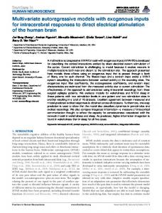
2. Methodology Initially, the ranking technique is applied to find the potential causes of at least 75% of the events registered in the historical time series of injured people in traffic accidents in Santiago de Chile. The causes related to drivers, pedestrians, and passengers behavior were prioritized. The forecasting methodology applied in the analyzed hybrid models is described in two stages, preprocessing and prediction, as Figure 1 illustrates. In the preprocessing stage Singular Spectrum Analysis and Singular Value Decomposition of Hankel are used to extract an additive component of low frequency from the observed time series, and by simple subtraction between the observed time series and the component of low frequency, the component of high frequency is obtained. In the prediction stage, linear and nonlinear models are implemented. 2.1. Singular Spectrum Analysis. Singular Spectrum Analysis extracts the component of low frequency 𝑐𝐿 from the observed time series. The component of high frequency 𝑐𝐻 is obtained by simple subtraction between the observed time series 𝑥 and the component 𝑐𝐿 . Consider 𝑐𝐻 = 𝑥 − 𝑐𝐿 .
(1)
Mathematical Problems in Engineering
3 𝑉𝑖 is the 𝑖th right singular vector of 𝑌. The collection √𝜆 𝑖 𝑈𝑖 𝑉𝑖 is called 𝑖th eigentriple of the SVD. The computation of the optimal window length 𝑟 is based on the eigenvalues differential entropy. The first 𝑡 eigenvalues obtained with 𝑟 = 𝑝/2 contain a high spread of energy; therefore, the window length is evaluated in the range [𝑟 = 2, . . . , 𝑡] by means of the differential entropy as follows:
x, r
Preprocessing HSVD
Preprocessing SSA
Embedding Y
A
Extraction HSVD
𝜆UV
Singular value decomposition
cL cL
A 𝜆UV Diagonal averaging
cH
AR or ANN
cL
cL
Δ𝐻𝑖 = 𝐻𝑖+1 − 𝐻𝑖 , 𝑖 = 1, . . . , 𝑡 − 1,
cH
𝑟
ĉL ĉ H
+
Conventional SSA is implemented in four steps, embedding, decomposition, grouping, and diagonal averaging [24]. In this work, SSA is simplified in three steps: embedding, decomposition, and diagonal averaging. The embedding step maps the time series 𝑥 of length 𝑝 to a sequence of multidimensional lagged vectors; the Hankel matrix structure is used in the embedding:
𝑌=(
⋅ ⋅ ⋅ 𝑥𝑞
𝑥2
𝑥3
⋅ ⋅ ⋅ 𝑥𝑞+1
.. .
.. .
.. .
.. .
),
(2)
(5c)
where Δ𝐻𝑖 is the 𝑖th differential entropy, 𝐻𝑖 is the 𝑖th Shannon entropy, and 𝜆𝑗 is the 𝑗th normalized eigenvalue also known as eigenvalue energy. The embedding step is executed again with this decomposition that reaches a high energy spread and lower differential entropy. With the optimal 𝑟 the embedding and decomposition are computed again. The first eigentriple is used to obtain the elementary matrix 𝐴, which will be used in the extraction of the low frequency component:
(3)
The Singular Value Decomposition of the real matrix 𝑌 has the form 𝑟
(4)
𝑖=1
where each 𝜆 𝑖 is the 𝑖th eigenvalue of the matrix 𝑆 = 𝑌𝑌⊤ arranged in decreasing order of magnitudes. 𝑈1 , . . . , 𝑈𝑟 is the corresponding orthonormal eigenvectors system of the matrix 𝑆. Standard SVD terminology calls √𝜆 𝑖 the 𝑖th singular value of the matrix 𝑌; 𝑈𝑖 is the 𝑖th left singular vector and
The step of diagonal averaging is applied over 𝐴 to extract the elements of the component 𝑐𝐿 ; the process is shown below:
1 𝑘 { { ∑ 𝐴 (𝑚, 𝑘 − 𝑚) , { { 𝑘 − 1 𝑚=1 { { { 𝑟 { {1 = { ∑ 𝐴 (𝑚, 𝑘 − 𝑚) , { 𝑟 𝑚=1 { { { 𝑟 { 1 { { ∑ 𝐴 (𝑚, 𝑘 − 𝑚) , { { 𝑞 + 𝑟 − 𝑘 + 1 𝑚=𝑘−𝑞
2 ≤ 𝑘 ≤ 𝑟, 𝑟 < 𝑘 ≤ 𝑞 + 1,
(7)
𝑞 + 2 ≤ 𝑘 ≤ 𝑞 + 𝑟.
Once 𝑐𝐿 is obtained, the component 𝑐𝐻 is computed with (1). 2.2. Hankel Singular Value Decomposition. The preprocessing based on Singular Value Decomposition of Hankel is implemented in three steps: embedding, decomposition, and extraction. HSVD implements the steps of embedding and decomposition as SSA (presented in Section 2.1). The elementary matrix 𝐴 is also computed with the first eigentriple obtained in the decomposition step (as (6)). In the extraction step, the elements of the low frequency component 𝑐𝐿 are obtained from the first row and the last column of the matrix 𝐴, which has the same structure as matrix 𝑌 (trajectory matrix); therefore, the elements of 𝑐𝐿 are
𝑐𝐿 = [𝐴 (1, 1) 𝐴 (1, 2) ⋅ ⋅ ⋅ 𝐴 (1, 𝑞) 𝐴 (2, 𝑞) 𝐴 (3, 𝑞) ⋅ ⋅ ⋅ 𝐴 (𝑟, 𝑞)] , where 𝐴 is a 𝑟 × 𝑞 matrix.
(6)
𝑐𝐿 (𝑖, 𝑗)
where the elements 𝑌(𝑖, 𝑗) = 𝑥𝑖+𝑗−1 . The window length 𝑟 has an important role in the forecasting model; it has an initial value of 𝑟 = 𝑝/2, and 𝑞 is computed as follows:
𝑌 = ∑√𝜆 𝑖 𝑈𝑖 𝑉𝑖⊤ ,
𝜆𝑗 , 𝑟 ∑𝑘=1 𝜆 𝑗
𝐴 = √𝜆 1 𝑈1 𝑉1⊤ .
(𝑥𝑟 𝑥𝑟+1 ⋅ ⋅ ⋅ 𝑥𝑝 )
𝑞 = 𝑝 − 𝑟 + 1.
(5b)
𝜆𝑗 =
Figure 1: Traffic accidents forecasting methodology.
𝑥2
𝐻𝑖 = − ∑𝜆𝑗 log2 𝜆𝑗 , 𝑗=1
̂ x
Prediction
𝑥1
(5a)
(8)
4
Mathematical Problems in Engineering
2.3. Prediction with the Autoregressive Method. The prediction is the second stage of the traffic accidents forecasting methodology (illustrated in Figure 1). In order to obtain the ̂ , during the preprocessing stage traffic accidents prediction 𝑥 the low frequency component 𝑐𝐿 and the high frequency component 𝑐𝐻 were obtained. The components are estimated through the autoregressive method and the addition of the components is computed to obtain the prediction as follows: 𝑛+ℎ ̂ 𝑛+ℎ = 𝑐̂𝐿 𝑛+ℎ + 𝑐̂ , 𝑥 𝐻
(9)
where 𝑛 represents the time instant and ℎ represents the horizon, with values ℎ = 1, . . . , 𝜏. The component 𝑐𝐿 is used as exogenous variable in the computation of the 𝑐𝐻, due to a high influence of 𝑐𝐿 over 𝑐𝐻. The predicted components via AR model are defined with 𝑐̂𝐿
𝑛+ℎ
=
𝑚−1
∑ 𝛼𝑖 𝑐𝐿𝑛−𝑖 , 𝑖=0
(10a)
𝑚−1
𝑚−1
𝑖=0
𝑖=0
𝑛+ℎ 𝑛−𝑖 = ∑ 𝛽𝑖 𝑐𝐻 + ∑ 𝛽𝑚+𝑖 𝑐𝐿𝑛−𝑖 , 𝑐̂ 𝐻
(10b)
where 𝑚 is the number of lagged values and 𝛼𝑖 and 𝛽𝑖 are the coefficients of 𝑐𝐿 and 𝑐𝐻, respectively. The coefficients estimation is based on linear Least Square Method (LSM); the components 𝑐𝐿 and 𝑐𝐻 are defined with the linear relationship expressed in matrix form: 𝑐𝐿 = 𝛼𝑅,
(11a)
𝑐𝐻 = 𝜃𝑍,
(11b)
where 𝑅 and 𝑍 are the regressor matrices of 𝑐𝐿 and 𝑐𝐻, respectively; 𝛼 and 𝜃 are the coefficients vectors of 𝑅 and 𝑍, respectively. The coefficients are computed with the MoorePenrose pseudoinverse matrices, 𝑅† and 𝑍† , as follows: 𝛼 = 𝑅† 𝑐𝐿 ,
(12a)
𝜃 = 𝑍† 𝑐𝐻.
(12b)
2.4. Prediction with the Autoregressive Neural Network. In this case study, a single hidden layer Autoregressive Neural Network is used to approach each component; the ANN has a standard multilayer perceptron (MLP) structure of three layers [28]. The training subset is iteratively used to adjust the connections weights via learning algorithm; the ANN with the lowest error is selected to implement the solution with the testing subset. The nonlinear inputs are the lagged terms, which are contained in the regressor matrix 𝑅; at hidden layer is applied the sigmoid transfer function, and at output layer is obtained the prediction. The ANN output is ̂ 𝑛+ℎ = V𝑗 ℎ𝑛+ℎ , 𝑥
(13a)
𝑚−1
ℎ𝑛+ℎ = 𝑓 [ ∑ 𝑤𝑗𝑖 𝑅𝑖𝑛+ℎ−𝑖 ] , 𝑖=0
(13b)
̂ is the predicted value, 𝑛 is the time instant, V𝑗 and 𝑤𝑗𝑖 where 𝑥 are the linear and nonlinear weights of the ANN connections, respectively; the sigmoid transfer function is computed with 𝑓 (𝑥) =
1 . 1 + 𝑒−𝑥
(14)
The ANN structure for 𝑐𝐿 prediction is denoted with ANN(𝑚, 𝑗, 1), with 𝑚 inputs, 𝑗 hidden nodes, and 1 output 𝑐̂𝐿 while the ANN structure for 𝑐𝐻 is denoted with ANN(2𝑚, 𝑗, 1), with 2𝑚 inputs, 𝑗 hidden nodes, and 1 output 𝑐̂ 𝐻 . Levenberg-Marquardt is the learning algorithm applied for weight updating in both neural networks [29].
3. Efficiency Criteria The forecasting accuracy is evaluated with conventional metrics and an improved evaluation metric. The conventional metrics are Mean Absolute Percentage Error (MAPE), Root Mean Square Error (RMSE), Determination Coefficient 𝑅2 , and Relative Error (RE). The Modified Nash-Sutcliffe Efficiency (MNSE) metric is computed in order to improve the evaluation criteria, which is sensitive to significant overfitting or underfitting [30]. Consider MAPE =
𝑝 ̂ 𝑖 1 𝑡 𝑥𝑖 − 𝑥 ∑ 100, 𝑝𝑡 𝑖=1 𝑥𝑖
RMSE = √
𝑝
1 𝑡 2 ̂𝑖) , ∑ (𝑥𝑖 − 𝑥 𝑝𝑡 𝑖=1
𝑅2 = [1 −
̂) var (𝑥 − 𝑥 ] 100, var (𝑥)
(15)
̂) (𝑥 − 𝑥 ] 100, 𝑥 𝑝 ̂ 𝑖 ∑ 𝑡 𝑥𝑖 − 𝑥 MNSE = [1 − 𝑖=1 𝑝𝑡 ] 100, ∑𝑖=1 𝑥𝑖 − 𝑥 RE = [
̂ is the predicted signal, 𝑝𝑡 is where 𝑥 is the observed signal, 𝑥 the testing sample size, and var is the variance. Furthermore, two statistical tests are computed to evaluate the differences and superiorities of either model, the Wilcoxon test and Pitman’s correlation test, respectively. The Wilcoxon (𝑊) signed rank test evaluates the pairwise differences in the squares of each multistep ahead residuals; the differences are ranked in ascending order, with no regard to the sign, and the ranks are assigned from one to the number of the forecast errors available for comparison. The sum of the ranks of positive differences is then computed to obtain 𝑊 [31]. The probability 𝑝 of finding a test statistic as or more extreme than the observed value under the null hypothesis is found using the 𝑍-statistics given by 𝑍=
𝑊 − 𝑝𝑡 (𝑝𝑡 + 1) /4 √𝑝𝑡 (𝑝𝑡 + 1) (2𝑝𝑡 + 1) /24
.
(16)
Mathematical Problems in Engineering
5
𝑅=
cov (Υ, Ψ) , var (Υ) var (Ψ)
(17a)
Υ = 𝐸1 (𝑖) + 𝐸2 (𝑖) ,
(17b)
Ψ = 𝐸1 (𝑖) − 𝐸2 (𝑖) ,
(17c)
where cov is the covariance and 𝑖 = 1, . . . , 𝑝𝑡 . 𝐸1 is the residual vector obtained with model 1, and 𝐸2 is the residual vector obtained with model 2. Model 1 would show superiority in front of model 2 at 5% significance level if |𝑅| > 1.96/√𝑝𝑡 .
4. Case Study The Chilean police (Carabineros de Chile) collects the features of the traffic accidents, and CONASET records the data. The regional population is estimated in 6,061,185 inhabitants, equivalent to 40.1% of the national population. Santiago shows a high rate of the events with severe injuries from 2000 to 2014, with 260,074 injured people. The entire series of 783 registers is shown in Figure 2, which have been collected in the mentioned period from January to December, with weekly sampling. The highest number of injured people was observed in weeks 84, 184, 254, and 280, while the lowest number of injured people was observed in weeks 344, 365, 426, 500, and 756. One hundred causes of traffic accidents have been defined by CONASET and grouped into categories. In this case study, three analysis groups have been created. In groups 1 and 2, those causes directly related to behavior of drivers, passengers, or pedestrians have been prioritized. Group 3 involves the rest of the causes. Figures 3(a), 4(a), and 5(a) show the observed time series of the groups, Injured-G1, Injured-G2, and Injured-G3, respectively; the values have been normalized via division by the maximum value in each time series. The categories of groups 1 and 2 are as follows: reckless driving, recklessness in passenger, recklessness in pedestrian, alcohol in driver, alcohol in pedestrian, and disobedience to signal. In Table 1 are shown 20 causes of groups 1 and 2, which cover 75% of the events with injured people. The causes are listed sequentially; the cause with the highest importance has value 1 (with the highest number of injured people), and the cause with minor importance has value 20. From Table 1, the first three causes of injuries in traffic accidents are as follows: unwise distance, inattention to traffic conditions, and disrespect to red light. The cause with the lowest importance for injuries in traffic accidents is drunk pedestrian. The categories with the highest number of causes are as follows: imprudent driving and disobedience to signal. Two groups of analysis were formed from the information presented in Table 1; the first group labeled with InjuredG1 corresponds to the first ten primary causes, and the second group labeled with Injured-G2 corresponds to the ten secondary causes. The first group overspreads around 60%
550 Number of injured people
Pitman’s correlations test is applied to identify the superiority of a model in pairwise comparisons [32]; the test is based on the computation of the correlation 𝑅 between Υ and Ψ as follows:
500 450 400 350 300 250 200 1 54 107 160 213 266 319 372 425 478 531 584 637 690 743 783 Time (weeks)
Figure 2: Injured people in traffic accidents.
of injured people in traffic accidents, whereas the second group overspreads around 15%. The third group, labeled with Injured-G3, corresponds to the categories road deficiencies, mechanical failures, and undetermined/noncategorized causes; this group overspreads around 25% of injured people. Complementary information was observed about traffic accidents conditions with high rate of injured people. With regard to vehicles, automobiles are involved in 54% of events, followed by vans and trucks with 19%, bus and trolley with 16%, motorcycles and bicycles with 8%, and others with 3%. With regard to environmental conditions, 85% of events was observed with cloudless conditions. Additionally, 97% of the traffic accidents with injured people have taken place in urban areas, whereas 3% correspond to rural area. With regard to relative position, 46% of the events have been produced in intersections controlled by traffic signals or police officers with 46%, followed by accidents that happened in straight sections with 37%, and other relative positions with 17%.
5. Empirical Research Result The results of the methodology implementation with linear and nonlinear models are described by stages: components extraction and prediction. 5.1. Components Extraction. The methodology presented in Section 2 describes the preprocessing stage and the prediction stage. The preprocessing stage is based on two types of methods, Singular Spectrum Analysis and Singular Value Decomposition of Hankel. Both preprocessing techniques SSA and HSVD embed the time series in a structure of two dimensions; the initial window length used is 𝑟 = 𝑝/2. Once matrix 𝑌 is obtained, the decomposition is computed. The differential energy of the eigenvalues is obtained with (5a). A high energy content was observed in the first 𝑡 = 20 eigenvalues; the lowest differential energy was observed in decompositions based on values of 15, 17, and 16 of window length, for Injured-G1, Injured-G2, and Injured-G3, respectively, and these values were set as window length. The embedding process is implemented again with the optimal window 𝑟, and the decomposition is recomputed. The first elementary matrix 𝐴 is used by SSA and HSVD to
6
Mathematical Problems in Engineering
0.8 0.6
0.6
cL
Injured-G1
1 0.8
0.4
0.4 0.2
0.2
1 53 105 157 209 261 313 365 417 469 521 573 625 677 729 783 Time (weeks)
1 53 105 157 209 261 313 365 417 469 521 573 625 677 729 783 Time (weeks) SSA HSVD
(a)
(b)
cH
0.5 0 −0.5 1 53 105 157 209 261 313 365 417 469 521 573 625 677 729 783 Time (weeks) SSA HSVD (c)
1 0.8 0.6 0.4 0.2 0
0.8 0.6 cL
Injured-G2
Figure 3: (a) Injured-G1. (b) Low frequency component. (c) High frequency component.
0.4 1 53 105 157 209 261 313 365 417 469 521 573 625 677 729 783
0.2 1 53 105 157 209 261 313 365 417 469 521 573 625 677 729 783
Time (weeks)
Time (weeks) SSA HSVD
(a)
(b)
0.4 cH
0.2 0 −0.2 −0.4
1 53 105 157 209 261 313 365 417 469 521 573 625 677 729 783 Time (weeks) SSA HSVD (c)
Figure 4: (a) Injured-G2. (b) Low frequency component. (c) High frequency component.
obtain the low frequency 𝑐𝐿 component. In SSA, to extract the elements of 𝐴, diagonal averaging is applied, while HSVD uses direct extraction from the first row and last column of 𝐴. Finally with (1) the component of high frequency 𝑐𝐻 was computed. Each data set of low and high frequency has been divided into two subsets, training and testing; the training subset
involves 70% of the samples, and consequently the testing subset involves the remaining 30%. The decomposition results by means of SSA and HSVD. Figures 3(b), 4(b), and 5(b) show the low frequency components, whereas Figures 3(c), 4(c), and 5(c) show the high frequency components of Injured-G1, Injured-G2, and Injured-G3, respectively.
Mathematical Problems in Engineering
7
Table 1: Causes of injuries in traffic accidents (group 1 and group 2). Category
Number 1 2 3 4 5 6 7 8 9 10 11 12 13 14 15 16 17 18 19 20
Imprudent driving
Disobedience to signal
Alcohol in driver
Recklessness in pedestrian
1 0.8 0.6 0.4 0.2
Importance 1 2 8 9 10 11 14 18 19 3 4 6 13 7 15 5 12 17 16 20
0.8 0.6 cL
Injured-G3
Recklessness in passenger Alcohol in pedestrian
Cause Unwise distance Inattention to traffic conditions Disrespect to pedestrian passing Disrespect for giving the right of way Unexpected change of track Improper turns Overtaking without enough time or space Opposite direction Backward driving Disrespect to red light Disrespect to stop sign Disrespect to give way sign Improper speed Drunk driver Driving under the influence of alcohol Pedestrian crossing the road suddenly Reckless pedestrian Pedestrian outside the allowed crossing Get in or get out of a moving vehicle Drunk pedestrian
0.4 0.2
1 53 105 157 209 261 313 365 417 469 521 573 625 677 729 783 Time (weeks)
1 53 105 157 209 261 313 365 417 469 521 573 625 677 729 783 Time (weeks) SSA HSVD
(a)
(b)
cH
0.5 0 −0.5 1 53 105 157 209 261 313 365 417 469 521 573 625 677 729 783 Time (weeks) SSA HSVD (c)
Figure 5: (a) Injured-G3. (b) Low frequency component. (c) High frequency component.
The nonstationary trend in the signals was verified for Injured-G1, Injured-G2, and Injured-G3 through Kwiatkowski, Phillips, Schmidt, and Shin test (KPSS) [33]. The test assesses the null hypothesis that the signals are trend stationary; it was rejected at 5% significance level; consequently, nonstationary unit-root processes are present in the signals.
The time series Injured-G1 is observed in Figure 3(a); similar dynamic is observed with respect to full series, taking into consideration that this group contains the predominant causes. The 𝑐𝐿 components extracted by SSA and HSVD are shown in Figure 3(b); long-memory periodicity features were observed. The 𝑐𝐻 resultant components are presented in
8 Figure 3(c); short-term periodic fluctuations were identified. The components obtained with SSA and HSVD are similar; however, a slight difference is observed in the components of low frequency; SSA extracts smoother components than HSVD. Both techniques SSA and HSVD show that the principal ten causes (in Table 1 with importance 1 to 10) present the highest incidence between years 2002 and 2005 (weeks 106 to 312); it descends from 2006 until half 2012 (around week 710); an increment is observed between weeks 711 and 732 (second semester of 2013 and first semester of 2014). Figure 4 shows the time series Injured-G2, the low frequency component, and the high frequency component. As previous series, the components of low frequency show similar dynamic of slow fluctuations with decreasing trend (𝑐𝐿 ), while the high frequency shows fast fluctuations. In this group is also observed 𝑐𝐿 via SSA smoother than 𝑐𝐿 via HSVD. Both techniques SSA and HSVD show that the secondary ten causes (described in Table 1 with importance 11 to 20) present the highest incidence of injured people in years 2000, 2003, and 2004; it descends from 2005; therefore, forward downtrend is observed in the number of injured people in traffic accidents due to the 10 secondary causes. Figure 5 shows Injured-G3 and its components 𝑐𝐿 and 𝑐𝐻; as in previous analysis the components of low frequency show long-memory periodicity features, whereas the components of high frequency show short-term periodic fluctuations, and 𝑐𝐿 via SSA is smoother than 𝑐𝐿 via HSVD. Both techniques SSA and HSVD show that the causes are related to road deficiencies, mechanical failures, and undetermined/noncategorized causes (with 25% of incidence). The highest incidence is observed in year 2001, from year 2002 it presents strong decay until 2006, and forward uptrend is observed with a temporal decrease in 2009. Prevention plans and punitive laws have been implemented in Chile during the analyzed period, via education, drivers licensing reforms, zero tolerance law, Emilia’s law, and transit law reforms, among others. The effect of a particular preventive or punitive action is not analyzed in this work; however, the proposed short-term prediction methodology based on observed causes and intrinsic components is a contribution to government and society in preventive plans formulation, its implementation, and the consequent evaluation. 5.2. Prediction. The prediction is implemented by means of the autoregressive models, linear (AR) or nonlinear (ANN). The models use the lagged terms of the components 𝑐𝐿 and 𝑐𝐻; the optimal number of the lagged terms was fixed in 𝑚 = 32 weeks, which was found through the computation of the Autocorrelation Function over the observed time series of injured people due to all causes. The models based on Singular Spectrum Analysis (SSAAR and SSA-ANN) receive the components of SSA preprocessing stage, whereas the models based on Singular Value Decomposition of Hankel (HSVD-AR and HSVD-ANN) receive the components of HSVD preprocessing stage. The ANN has single hidden layer structure (32, 1, 1), with 32 inputs, 1 hidden node, and 1 output. The LM algorithm was used iteratively to adjust the linear and nonlinear weights.
Mathematical Problems in Engineering The direct method was used to develop multistep ahead forecasting; in Tables 2 and 3 are presented the average prediction results with hybrid models SSA-AR, SSA-ANN, HSVD-AR, and HSVD-ANN with the three time series. The arithmetic mean of the resultant metrics is presented in Tables 2 and 3; the results shows that the accuracy decreases as the time horizon increases; therefore, the best accuracy was obtained for the nearest weeks, and the lowest accuracy was obtained for the farthest weeks. The best mean accuracy was reached by using SSA-AR model, with MNSE of 92.6%, 𝑅2 of 99.3%, MAPE of 1.5%, and RMSE of 0.7%. The lowest mean accuracy was obtained with HSVD-ANN model, with MNSE of 85.6%, 𝑅2 of 98.2%, MAPE of 2.9%, and RMSE of 1.4%. The second best average accuracy was reached by SSA-ANN, and the third best accuracy was reached by HSVD-AR. The highest gain in average MNSE from 1- to 14-step ahead prediction is 7.6%, while average MAPE is 93.3%. However, it was observed that HSVD-AR shows a higher accuracy in farthest horizons, from 12- to 14-step ahead prediction, which reaches these average results: MNSE of 89.4%, 𝑅2 of 98.9%, MAPE of 2.2%, and of RMSE 1.0%; the gain in average MNSE from 12- to 14-step ahead prediction is 12.1%, and on average MAPE is 83.3%. Prediction horizons higher than 14 weeks provide inaccurate results. From previous tables, similar accuracy was identified in the prediction through SSA-AR, HSVD-AR, and SSA-ANN, for 11-step ahead prediction. The predicted signals are shown in Figures 6, 7, and 8, whereas the metrics residuals are presented in Tables 4, 5, and 6. The results for 11-step ahead prediction of Injured-G1 are shown in Figures 6(a), 6(c), 6(e), and Table 4. From these figures and metrics, a good fit is observed; the highest accuracy was reached via SSA-AR with MNSE of 87.6%, 𝑅2 of 98.6%, MAPE of 2.0%, and RMSE of 1.1%. In Figures 6(b), 6(d), and 6(f), the Relative Error of Injured-G2 prediction is shown. The model SSA-AR shows 94.7% of the predicted points with Relative Error lower than ±5%, HSVD-AR 86.7%, and SSA-ANN 83.1%. The gain was computed by means of residual metrics and the two best models (SSA-AR and HSVD-AR); the highest gain was observed in MAPE with 25%. The results for 11-step ahead prediction of Injured-G2 are shown in Figures 7(a), 7(c), and 7(e) and Table 5; all models achieve a good fit; SSA-AR and HSVD-AR reach the highest and similar accuracy. In Figures 7(b), 7(d), and 7(f), the Relative Error is shown; SSA-AR presents 85.8% of the predicted points with a Relative Error lower than ±5%, HSVD-AR 85.3%, and SSA-ANN 80%. The gain was computed based on residual metrics and the two best models; the highest gain was observed in MAPE with 10.7%. The results for 11-step ahead prediction of Injured-G3 are presented in Figures 8(a), 8(c), and 8(e) and Table 6; all models achieve also a good fit and similar accuracy. In Figures 8(b), 8(d), and 8(f), the Relative Error is illustrated; SSA-AR presents 92.4% of predicted points with a Relative Error lower than ±5%, HSVD-AR 94.2%, and SSA-ANN 91.6%. The gain
Mathematical Problems in Engineering
9
Table 2: Multistep ahead prediction—average results, MNSE, and 𝑅2 . ℎ (week) 1 2 3 4 5 6 7 8 9 10 11 12 13 14 Min Max Mean 1–14 steps Mean 12–14 steps
SSA-AR 99.5 98.8 97.9 96.9 95.8 94.6 93.4 92.2 90.9 89.6 88.4 87.2 86.2 85.3 85.3 99.5 92.6 86.2
MNSE (%) SSA-ANN HSVD-AR 99.4 96.4 98.7 94.6 97.6 93.2 96.7 91.7 95.3 90.6 93.6 89.4 92.6 88.2 91.3 87.5 89.4 87.4 87.9 87.4 86.3 87.6 84.5 88.6 77.3 89.0 73.9 90.5 73.9 87.4 99.4 96.4 90.3 90.1 78.6 89.4
HSVD-ANN 95.7 93.1 90.9 89.2 86.9 85.2 83.5 81.9 80.2 81.7 82.2 86.6 83.4 77.3 77.4 95.7 85.6 82.4
SSA-AR 99.9 99.9 99.9 99.9 99.8 99.7 99.6 99.4 99.2 99.0 98.8 98.5 98.3 98.1 98.1 99.9 99.3 98.3
𝑅2 (%) SSA-ANN HSVD-AR 99.9 99.9 99.9 99.7 99.9 99.6 99.9 99.4 99.8 99.2 99.7 99.0 99.5 98.8 99.3 98.6 99.1 98.5 98.8 98.5 98.5 98.6 98.2 98.7 96.7 98.9 95.9 99.1 95.9 98.5 99.9 99.9 98.9 99.0 96.9 98.9
HSVD-ANN 99.8 99.6 99.3 98.9 98.6 98.3 97.7 97.4 97.5 97.6 97.2 98.5 97.9 96.6 96.6 99.8 98.2 97.7
Table 3: Multistep ahead prediction—average results, MAPE, and RMSE. ℎ (week) 1 2 3 4 5 6 7 8 9 10 11 12 13 14 Min Max Mean 1–14 steps Mean 12–14 steps
SSA-AR 0.1 0.3 0.4 0.6 0.9 1.1 1.3 1.6 1.8 2.1 2.4 2.6 2.9 3.1 0.1 3.1 1.5 2.9
MAPE (%) SSA-ANN HSVD-AR 0.1 0.8 0.3 1.1 0.5 1.4 0.7 1.7 1.0 1.9 1.3 2.2 1.5 2.4 1.8 2.6 2.3 2.6 2.5 2.6 2.9 2.5 3.3 2.3 4.1 2.3 4.7 2.0 0.1 0.8 4.7 2.6 1.9 2.0 4.0 2.2
HSVD-ANN 0.9 1.4 1.8 2.2 2.8 3.1 3.5 3.7 3.8 3.8 3.8 2.9 3.5 4.2 0.9 4.2 2.9 3.5
was computed based on residual metrics and the two best models; the highest gain was observed in RMSE with 7.7%. In the next section the differences and/or superiorities of either linear model SSA-AR or HSVD-AR are identified through the application of the statistical tests. 5.3. Models Statistical Tests. The performance of the linear hybrid models SSA-AR and HSVD-AR is evaluated with
SSA-AR 0.05 0.13 0.21 0.30 0.40 0.52 0.64 0.76 0.88 1.0 1.1 1.2 1.3 1.4 0.05 1.4 0.7 1.3
RMSE (%) SSA-ANN HSVD-AR 0.05 0.36 0.13 0.54 0.22 0.67 0.32 0.79 0.45 0.89 0.6 0.99 0.7 1.11 0.8 1.19 0.9 1.22 1.1 1.22 1.3 1.18 1.4 1.13 2.0 1.06 2.3 0.91 0.06 0.36 2.3 1.22 0.9 1.0 1.9 1.0
HSVD-ANN 0.43 0.67 0.87 1.03 1.23 1.37 1.59 1.70 1.72 2.19 2.18 1.34 1.98 2.07 0.4 2.2 1.4 1.8
the Wilcoxon hypothesis test and with Pitman’s correlations test ((16)–(17a), (17b), and (17c)). The Wilcoxon hypothesis test results are shown in Table 7, and Pitman’s correlation test results are shown in Table 8. From Table 7, in 37 comparisons between residuals of SSA-AR and HSVD-AR, the test rejects the null hypothesis that there is no difference in the prediction at 5% significance level. In the remaining 5 comparisons the null hypothesis that
10
Mathematical Problems in Engineering 1
10 6 Rel. error (±5%)
Injured-G1
0.8 0.6 0.4
2 −2 −6 −10
0.2 1
33
65
97
129
161
193
220
1
33
Testing sample (weeks)
65 97 129 161 Testing sample (weeks)
193
220
Observed SSA-AR (b)
(a)
10
1
6 Rel. error (±5%)
Injured-G1
0.8 0.6 0.4
2 −2 −6 −10
0.2 1
33
65
97
129
161
193
1
220
33
161
193
220
65 97 129 161 Testing sample (weeks)
193
220
65
97
129
Testing sample (weeks)
Testing sample (weeks) Observed HSVD-AR
(d)
(c)
10
1
6 Rel. error (±5%)
Injured-G1
0.8
0.6
0.4
2 −2 −6 −10
0.2 1
33
65
97 129 161 Testing sample (weeks)
193
220
1
33
Observed SSA-ANN (e)
(f)
Figure 6: Injured-G1 11-step ahead prediction. (a) SSA-AR Prediction. (b) SSA-AR Relative Error. (c) HSVD-AR Prediction. (d) HSVD-AR Relative Error. (e) SSA-ANN Prediction. (f) SSA-ANN Relative Error.
there is no difference in the prediction is accepted. In this case, there is no difference in 12-step ahead prediction for time series Injured-G1; the same situation was found in 10and 11-step ahead prediction for time series Injured-G2 and Injured-G3. Pitman’s correlations test is applied with the residual values to identify the superiority of SSA-AR over HSVD-AR
or the opposite. The correlations between Υ and Ψ are shown in Table 8. The null hypothesis of Pitman’s correlation is true at 5% significance level if |𝑅| > 1.96/√𝑝𝑡 , where 𝑝𝑡 = 225 testing samples. The results of the correlations are shown in Table 8. From Table 8, the results present similarities with respect to Wilcoxon test. In 5 predictions there is no superiority of either
11
1
10
0.8
6
Rel. error (±5%)
Injured-G2
Mathematical Problems in Engineering
0.6 0.4 0.2 0 1
33
65
97 129 161 Testing sample (weeks)
193
2 −2 −6 −10
220
1
33
65 97 129 161 Testing sample (weeks)
193
220
193
220
193
220
Observed SSA-AR (b)
10
0.8
6
Rel. error (±5%)
Injured-G2
(a)
1
0.6 0.4 0.2 0
2 −2 −6 −10
1
33
65
97
129
161
193
1
220
33
Testing sample (weeks)
65 97 129 161 Testing sample (weeks)
Observed HSVD-AR (d)
1
10
0.8
6
Rel. error (±5%)
Injured-G2
(c)
0.6 0.4 0.2
2 −2 −6 −10
0 1
33
65
97 129 161 Testing sample (weeks)
193
1
220
33
65 97 129 161 Testing sample (weeks)
Observed SSA-ANN (f)
(e)
Figure 7: Injured-G2 11-step ahead prediction. (a) SSA-AR Prediction. (b) SSA-AR Relative Error. (c) HSVD-AR Prediction. (d) HSVD-AR Relative Error. (e) SSA-ANN Prediction. (f) SSA-ANN Relative Error.
Table 5: 11-step ahead prediction results, Injured-G2.
Table 4: 11-step ahead prediction results, Injured-G1.
MNSE 𝑅2 MAPE RMSE RE ± 5%
SSA-AR 87.6 98.6 2.0 1.1 94.7
HSVD-AR 84.7 98.0 2.5 1.3 86.7
SSA-ANN 82.9 98.0 3.1 1.5 83.1
Gain 3.3% 0.6% 25% 18.2% 8.4%
model (SSA-AR and HSVD-AR). SSA-AR shows superiority with respect to HSVD-AR in 30 predictions (when |𝑅| > 0.123 for nearest horizons), whereas the opposite is observed
MNSE 𝑅2 MAPE RMSE RE ± 5%
SSA-AR 90.3 99.1 2.8 0.9 85.8
HSVD-AR 90.6 99.1 2.5 0.9 85.3
SSA-ANN 88.4 98.7 3.6 1.0 80.0
Gain 0.3% 0% 10.7% 0% 0.6%
in 7 predictions; HSVD-AR shows superiority with respect to SSA-AR (when |𝑅| ≤ 0.123 for farthest horizons).
12
Mathematical Problems in Engineering 1
10 Rel. error (±5%)
Injured-G3
0.9
0.7
0.5
0.3
6 2 −2 −6 −10
1
33
65
97
129
161
193
1
220
33
Testing sample (weeks)
65 97 129 161 Testing sample (weeks)
193
220
193
220
193
220
Observed SSA-AR (b)
(a)
1
10 Rel. error (±5%)
Injured-G3
0.9 0.7 0.5
6 2 −2 −6 −10
0.3 1
33
65
97 129 161 Testing sample (weeks)
193
1
220
33
65 97 129 161 Testing sample (weeks)
Observed HSVD-AR (c)
(d)
1
10 6 Rel. error (±5%)
Injured-G3
0.9
0.7
0.5
2 −2 −6
0.3
−10 1
33
65
97 129 161 Testing sample (weeks)
193
220
1
33
65 97 129 161 Testing sample (weeks)
Observed SSA-ANN (f)
(e)
Figure 8: Injured-G3 11-step ahead prediction. (a) SSA-AR Prediction. (b) SSA-AR Relative Error. (c) HSVD-AR Prediction. (d) HSVD-AR Relative Error. (e) SSA-ANN Prediction. (f) SSA-ANN Relative Error.
6. Conclusions
Table 6: 11-step ahead prediction results, Injured-G3.
MNSE 𝑅2 MAPE RMSE RE ± 5%
SSA-AR 87.2 98.6 2.3 1.4 92.4
HSVD-AR 87.6 98.7 2.3 1.3 94.2
SSA-ANN 87.6 98.7 2.3 1.4 91.6
Gain 0.5% 0.1% 0% 7.7% 1.9%
In this paper has been developed multistep ahead traffic accidents forecasting approach based on singular values and autoregressive models. The nonstationary and nonlinear time series of injured people in traffic accidents of Santiago de Chile was used. Before the models methodology stages, ranking was applied to detect the relevant causes of injuries in traffic
Mathematical Problems in Engineering
13
Table 7: Wilcoxon hypothesis test—pairwise differences between SSA-AR and HSVD-AR. Series 1 2 3
1 1 1 1
2 1 1 1
3 1 1 1
4 1 1 1
5 1 1 1
6 1 1 1
7 1 1 1
Horizon 8 1 1 1
9 1 1 1
10 1 0 0
11 1 0 0
12 0 1 1
13 1 1 1
14 1 1 1
Table 8: Pitman’s correlation test 𝑅—pairwise comparisons between SSA-AR and HSVD-AR. Series 1 2 3
1 −0.9 −0.9 −0.9
2 −0.9 −0.9 −0.9
3 −0.9 −0.9 −0.9
4 −0.8 −0.8 −0.8
5 −0.8 −0.7 −0.7
6 −0.7 −0.6 −0.6
accidents; causes related to behavior of drivers, pedestrians, or passengers are predominant. Unwise distance, inattention to traffic conditions, and disrespect to red light are the first important causes of injuries in traffic accidents in concordance with previous studies that determine disrespect towards the road signs as a principal cause of traffic accidents. Complementary information was observed about traffic accidents conditions with high rate of injured people, automobiles type, environmental conditions, and relative position, among others. This approach was described in two stages, preprocessing and prediction; in the first stage two methods for components extraction were developed, Singular Spectrum Analysis and Singular Value Decomposition of Hankel, whereas in the second stage the linear autoregressive model and an Autoregressive Neural Network with Levenberg-Marquardt algorithm were used. Four hybrid models were implemented: SSA-AR, HSVDAR, SSA-ANN, and HSVD-ANN. The models were evaluated for 14-week ahead forecasting; comparative analysis shows that the proposed models SSA-AR and SSA-ANN achieved the highest accuracy with an average MNSE of 92.6% and 90.3%, respectively; the highest gain in average MNSE achieved by SSA-AR is 7.6%. However, it was observed that HSVD-AR shows a higher accuracy in farthest horizons from 12 to 14 steps, which reaches an average MNSE of 89.4%; in this case the highest gain achieved by HSVD-AR in MNSE is 12%. The statistical tests application through Wilcoxon and Pitman has shown that SSA-AR is superior to HSVD-AR in 30 of 42 comparisons of resultant efficiency criteria (at nearest horizon) at 5% significance level, 5 comparisons show equivalence, and 7 comparisons show the superiority of HSVD-AR over SSA (at farthest horizon). In further works, more strategies of components extraction will be explored; spectral analysis could help to explain the nature of traffic accidents in other geographic zones. Detailed work focused on the causes of traffic accidents will be done to support prevention plans aimed at promoting good habits on roads and highways.
Horizon 7 8 −0.6 −0.6 −0.5 −0.5 −0.5 −0.4
9 −0.5 −0.3 −0.3
10 −0.4 −0.2 −0.1
11 −0.2 0.0 0.0
12 −0.1 0.2 0.2
13 0.1 0.3 0.3
14 0.3 0.5 0.5
Competing Interests The authors declare that they have no competing interests regarding the publication of this paper.
References [1] World Health Organization, 2015, http://www.who.int. [2] J. Abell´an, G. L´opez, and J. de O˜na, “Analysis of traffic accident severity using decision rules via decision trees,” Expert Systems with Applications, vol. 40, no. 15, pp. 6047–6054, 2013. [3] L.-Y. Chang and J.-T. Chien, “Analysis of driver injury severity in truck-involved accidents using a non-parametric classification tree model,” Safety Science, vol. 51, no. 1, pp. 17–22, 2013. [4] J. De O˜na, G. L´opez, R. Mujalli, and F. J. Calvo, “Analysis of traffic accidents on rural highways using Latent Class Clustering and Bayesian Networks,” Accident Analysis and Prevention, vol. 51, pp. 1–10, 2013. [5] Y.-R. Shiau, C.-H. Tsai, Y.-H. Hung, and Y.-T. Kuo, “The application of data mining technology to build a forecasting model for classification of road traffic accidents,” Mathematical Problems in Engineering, vol. 2015, Article ID 170635, 8 pages, 2015. [6] L. Lin, Q. Wang, and A. W. Sadek, “A novel variable selection method based on frequent pattern tree for real-time traffic accident risk prediction,” Transportation Research Part C: Emerging Technologies, vol. 55, pp. 444–459, 2015. [7] M. Deublein, M. Schubert, B. T. Adey, J. K¨ohler, and M. H. Faber, “Prediction of road accidents: a Bayesian hierarchical approach,” Accident Analysis and Prevention, vol. 51, pp. 274– 291, 2013. [8] S. Ognjenovic, R. Donceva, and N. Vatin, “Dynamic homogeneity and functional dependence on the number of traffic accidents, the role in urban planning,” in Proceedings of the International Scientific Conference Urban Civil Engineering and Municipal Facilities (SPbUCEMF ’15), vol. 117, p. 551, 2015. [9] K. Keay and I. Simmonds, “Road accidents and rainfall in a large Australian city,” Accident Analysis and Prevention, vol. 38, no. 3, pp. 445–454, 2006. [10] M. Aron, R. Billot, N. E. Faouzi, and R. Seidowsky, “Traffic indicators, accidents and rain: some relationships calibrated on
14
[11] [12]
[13]
[14]
[15]
[16]
[17]
[18]
[19]
[20]
[21]
[22]
[23] [24] [25] [26]
[27]
[28]
Mathematical Problems in Engineering a French urban motorway network,” Transportation Research Procedia, vol. 10, pp. 31–40, 2015. Comisi´on Nacional de Seguridad de Tr´ansito, 2015, http://www .conaset.cl. H. Viljoen and D. G. Nel, “Common singular spectrum analysis of several time series,” Journal of Statistical Planning and Inference, vol. 140, no. 1, pp. 260–267, 2010. C. A. F. Marques, J. A. Ferreira, A. Rocha et al., “Singular spectrum analysis and forecasting of hydrological time series,” Physics and Chemistry of the Earth, Parts A/B/C, vol. 31, no. 18, pp. 1172–1179, 2006. L. Telesca, M. Lovallo, A. Shaban, T. Darwich, and N. Amacha, “Singular spectrum analysis and Fisher-Shannon analysis of spring flow time series: An application to Anjar Spring, Lebanon,” Physica A, vol. 392, no. 17, pp. 3789–3797, 2013. H. Hassani, S. Heravi, and A. Zhigljavsky, “Forecasting European industrial production with singular spectrum analysis,” International Journal of Forecasting, vol. 25, no. 1, pp. 103–118, 2009. H. Hassani, A. Webster, E. S. Silva, and S. Heravi, “Forecasting U.S. tourist arrivals using optimal singular spectrum analysis,” Tourism Management, vol. 46, pp. 322–335, 2015. J. Wang, S. Jin, S. Qin, and H. Jiang, “Swarm intelligencebased hybrid models for short-term power load prediction,” Mathematical Problems in Engineering, vol. 2014, Article ID 712417, 17 pages, 2014. H. Li, L. Cui, and S. Guo, “A hybrid short-term power load forecasting model based on the singular spectrum analysis and autoregressive model,” Advances in Electrical Engineering, vol. 2014, Article ID 424781, 7 pages, 2014. W. Zhang, Z. Su, H. Zhang, Y. Zhao, and Z. Zhao, “Hybrid wind speed forecasting model study based on SSA and intelligent optimized algorithm,” Abstract and Applied Analysis, vol. 2014, Article ID 693205, 14 pages, 2014. Y. Xiao, J. J. Liu, Y. Hu, Y. Wang, K. K. Lai, and S. Wang, “A neuro-fuzzy combination model based on singular spectrum analysis for air transport demand forecasting,” Journal of Air Transport Management, vol. 39, pp. 1–11, 2014. M. Abdollahzade, A. Miranian, H. Hassani, and H. Iranmanesh, “A new hybrid enhanced local linear neuro-fuzzy model based on the optimized singular spectrum analysis and its application for nonlinear and chaotic time series forecasting,” Information Sciences, vol. 295, pp. 107–125, 2015. L. Barba, N. Rodr´ıguez, and C. Montt, “Smoothing strategies combined with ARIMA and neural networks to improve the forecasting of traffic accidents,” The Scientific World Journal, vol. 2014, Article ID 152375, 12 pages, 2014. G. H. Golub and C. F. V. Loan, Matrix Computations, The Johns Hopkins University Press, 1996. N. Golyandina, V. Nekrutkin, and A. A. Zhigljavsky, Analysis of Time Series Structure, Chapman & Hall/CRC, 2001. J. Elsner and A. Tsonis, Singular Spectrum Analysis: A New Tool in Time Series Analysis, Plenum, 1996. H. Hassani, R. Mahmoudvand, and M. Zokaei, “Separability and window length in singular spectrum analysis,” Comptes Rendus Mathematique, vol. 349, no. 17-18, pp. 987–990, 2011. R. Wang, H.-G. Ma, G.-Q. Liu, and D.-G. Zuo, “Selection of window length for singular spectrum analysis,” Journal of the Franklin Institute, vol. 352, no. 4, pp. 1541–1560, 2015. J. A. Freeman and D. M. Skapura, Neural Networks, Algorithms, Applications, and Programming Techniques, Addison-Wesley, 1991.
[29] M. Hagan, H. Demuth, and M. Bealetitle, Neural Network Design, Hagan Publishing, 2002. [30] P. Krause, D. P. Boyle, and F. B¨ase, “Comparison of different efficiency criteria for hydrological model assessment,” Advances in Geosciences, vol. 5, pp. 89–97, 2005. [31] R. L. Ott and M. Longnecker, An Introduction to Statistical Methods and Data Analysis, Cengage Learning, Boston, Mass, USA, 6th edition, 2001. [32] K. Hipel and A. McLeod, Time Series Modelling of Water Resources and Environmental Systems, Elsevier, 1994. [33] D. Kwiatkowski, P. C. B. Phillips, P. Schmidt, and Y. Shin, “Testing the null hypothesis of stationarity against the alternative of a unit root: how sure are we that economic time series have a unit root?” Journal of Econometrics, vol. 54, no. 1–3, pp. 159–178, 1992.
Advances in
Operations Research Hindawi Publishing Corporation http://www.hindawi.com
Volume 2014
Advances in
Decision Sciences Hindawi Publishing Corporation http://www.hindawi.com
Volume 2014
Journal of
Applied Mathematics
Algebra
Hindawi Publishing Corporation http://www.hindawi.com
Hindawi Publishing Corporation http://www.hindawi.com
Volume 2014
Journal of
Probability and Statistics Volume 2014
The Scientific World Journal Hindawi Publishing Corporation http://www.hindawi.com
Hindawi Publishing Corporation http://www.hindawi.com
Volume 2014
International Journal of
Differential Equations Hindawi Publishing Corporation http://www.hindawi.com
Volume 2014
Volume 2014
Submit your manuscripts at http://www.hindawi.com International Journal of
Advances in
Combinatorics Hindawi Publishing Corporation http://www.hindawi.com
Mathematical Physics Hindawi Publishing Corporation http://www.hindawi.com
Volume 2014
Journal of
Complex Analysis Hindawi Publishing Corporation http://www.hindawi.com
Volume 2014
International Journal of Mathematics and Mathematical Sciences
Mathematical Problems in Engineering
Journal of
Mathematics Hindawi Publishing Corporation http://www.hindawi.com
Volume 2014
Hindawi Publishing Corporation http://www.hindawi.com
Volume 2014
Volume 2014
Hindawi Publishing Corporation http://www.hindawi.com
Volume 2014
Discrete Mathematics
Journal of
Volume 2014
Hindawi Publishing Corporation http://www.hindawi.com
Discrete Dynamics in Nature and Society
Journal of
Function Spaces Hindawi Publishing Corporation http://www.hindawi.com
Abstract and Applied Analysis
Volume 2014
Hindawi Publishing Corporation http://www.hindawi.com
Volume 2014
Hindawi Publishing Corporation http://www.hindawi.com
Volume 2014
International Journal of
Journal of
Stochastic Analysis
Optimization
Hindawi Publishing Corporation http://www.hindawi.com
Hindawi Publishing Corporation http://www.hindawi.com
Volume 2014
Volume 2014