Hybrid Stochastic Framework for Freeway Traffic Flow Modelling Lyudmila Mihaylova SYSTeMS, Universiteit Gent B-9052 Zwijnaarde, Belgium
[email protected]
Ren´e Boel SYSTeMS, Universiteit Gent B-9052 Zwijnaarde, Belgium
[email protected]
Abstract Traffic flow is an interesting many-particle phenomenon, with nonlinear interactions between the vehicles. This paper studies highway traffic and presents a general framework for traffic modelling as a stochastic hybrid system (with continuous and discrete dynamics and some interactions between its components). The freeway is considered as a network of components, each component modelling a different section of the traffic network. A model is developed in order to design stochastic predictors of the flows. The different traffic modes and transitions between them are detected and analyzed in real data, collected by induction loop detectors from Belgian and Dutch freeways.
1
Motivation
A freeway network consists of many interacting components. Traffic flow on each component is a complex system, with highly variable demand patterns, traffic jams, stop-and-go waves and hysteresis phenomena. Experimental studies [6, 7, 9, 10] based on traffic data have shown that traffic flow in different sections of a freeway possesses distinct dynamic modes (phases), such as: free flow traffic that is similar to the laminar flow in fluid systems: cars do not interact much with each other and each car approaches its own desired speed; synchronized traffic flow, a mode in which drivers move with nearly the same speed on the different lanes of the highway; congested mode in which the speed is quite low and can fluctuate very much while flow does not vary significantly; and jammed mode, where vehicles almost do not move and the flow is very low. Some changes in the section mode, for example from “free flow” to “congested”, are induced by the traffic dynamics themselves, while others are due to external events such as accidents, road works or weather conditions. We model the freeway traffic as a network of dynamic components, each component representing a different section of the network. The traffic is a stochastic hybrid system, i.e. each section is presented as a system with continuous and discrete states, interactions with variables of neighboring sections, and some unexpected abrupt changes in its modes. The continuous variables in a section are the flow through the boundary of the section,
Copyright held by the author
372
the average speed and the average density. Discrete state variables in a section are the number of lanes, traffic modes (free flow, synchronized, congested, jammed) and external conditions like weather. The traffic dynamics is described in this model by macroscopic variables, i.e. in terms of the collective vehicle dynamics, by aggregated variables and treating the traffic as a fluid flow. Various macroscopic models have been developed over the last 60 years for the deterministic or stochastic evolution of the three main variables of aggregated traffic: flow, speed, and density (for a recent survey, see [2, 3, 5, 8, 7]). The majority of the proposed in the literature macroscopic models are deterministic. Until now macroscopic models are predominantly used to simulate the traffic dynamics, less for traffic states estimation and control. Compared to the other types of models with higher level of details, such as microscopic (particle-based) and mesoscopic (gas-kinetic) [3], the macroscopic (fluid-dynamic) models are more suitable for the on-line description of traffic states in order to make predictions with real data. These predictions are then useful for model based feedback control, which is the ultimate motivation of our work. The remainder of the paper is organized as follows. Section 2 presents the framework for modelling of the traffic flow as a stochastic hybrid system. The freeway network is divided into components. Each component is described by its dynamic mode and by aggregated traffic variables. Section 3 is focussed on analysis of the transitions between different traffic modes and their on-line detection, based on real data from freeways. Finally, conclusions are given in Section 4.
2
Traffic Flow Considered as a Hybrid System
The network of freeways under study is divided into many sections, as indicated in Fig. 1. Each section corresponds to a stretch of a freeway where the behavior is fairly homogeneous. The traffic vehicular flow on the freeways is described as a stochastic hybrid system xi,k+1 = fi (xdi,k , xi−1,k , xi,k , xi+1,k , di,k , ηi,k ),
(1)
where the state vector xi,k = (ρi,k , vi,k )T contains the average traffic density (the number of vehicles per length unit, [veh/km]) and the average speed, [km/h]. The state vector xi,k+1 of the i-th section at time k + 1 is a function of state vectors at time k, from the i-th, and neighbor sections, i − 1 and i + 1. xi,k contains the continuously evolving variables at several equidistant points along the stretch of the freeway; x di,k = m is the vector of discrete variables (e.g. the number of lanes, the traffic mode, the weather) that describes a particular traffic mode; di,k is the vector of demands (on-ramp and offramp flows); ηi,k is a disturbance vector, with a known probability distribution pηi,k (ηi ). ηi,k reflects the fluctuations in the speed selected by different drivers under the same conditions. The traffic mode makes sudden transitions, jumps to a different mode with a rate that depends on xi,k , xi+1,k . Using traffic modes as discrete state variables allows for much simpler form of fi (e.g. affine function). In the first and the last zone of a section, di,k acts as a part of boundary conditions. These first and last zones are special because they describe boundary conditions, including the interaction with upstream and downstream sections, on- and off-ramps, etc.
373
Section i
ρi −1
qi −1 vi −1
qi
ρi
vi
ρi +1
Figure 1: Freeway divided per sections. The flow qi and the speed vi are at the outflow boundary, ρi is within the section. The measurement equation is of the form zi,k = hi (xi,k , ξi,k ),
(2)
where the measurement vector zi,k = (qi,k , vi,k )T comprises the average flow (the number of vehicles: cars and trucks, passing a specific location in a time unit, [veh/h]) and the average speed, measured by induction loop detectors at the boundary between some sections. The data are averaged over an interval of fixed length, e.g. one minute. They are corrupted by noise due to sensor calibration errors, communication link errors, sensor failures. The measurement noise ξi,k is assumed uncorrelated with di,k and ηi,k , with a known probability distribution pξi,k (ξi ). Functions fi and hi are nonlinear in general. We are building up efficient hybrid traffic models (with continuous and discrete components and some interaction between them) in order to solve the problems of: i ) estimation of the traffic variables, i.e. in finding of E(xk /Z k ) by using all available information, Z k = {zj,l , ∀ j = 1, 2, . . . , i, . . . , N, l = 1, 2, . . . , k} from N sections, and ii ) prediction of a future state, i.e. E(xk+1 /Z k ), where xk stacks all vectors xi,k , E(.) denotes the mathematical expectation operator. The posterior probability density function of the state P (xk /Z k ) is recursively updated from the sensor information, using the state update and the measurement update steps, aiming respectively the computation of the probability density functions P (xk+1 /xk ) and P (Z k /xk ). The recursive Bayesian approach is a suitable framework (e.g. particle filtering [1]). One of the challenges in these tasks is the need for on-line solutions, quickly after a new observations come in.
3
Traffic Analysis and Classification of its Modes
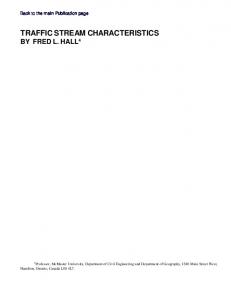
We investigate the transitions between the traffic modes empirically and theoretically. The traffic phenomenon is analyzed taking into account various upstream and downstream conditions and after splitting up the data according to the different phases. The data are collected from Belgian and Dutch freeways, respectively in June 2001 and August 2002. The transitions between the different modes may happen in a very irregular way: for instance the transition between free flow and synchronized traffic is of hysteretic nature, which means that the inverse transition from congested to free flow traffic occurs at a lower density and at a higher speed [4, 7]. On the basis of our analysis of the traffic data, and in agreement with the results of [7], we distinguish the following major modes: free flow (Fig. 2a), synchronized (Fig. 2b),
374
100 90 80 70 60
0
10
20
120
2000
110
1500 1000 500 0
30
10
100
80
6.5
7
7.5
20
90 80
1
8
140
2000
120
1500 1000 500
10
20
6.5
Time, [h]
7
7.5
1
1000
3
30
5
8
8.5
10
15
20
25
30
Density, [veh/km] 3000
3
2
100 80 60
1
2
1
2500 2000 1500 1000 500
3
40 6
1500
Density, [veh/km]
2500
0 5.5
8.5
2000
500
60
30
Speed, [km/h]
Flow, [veh/h]
Speed, [km/h]
120
6
100
Density, [veh/km]
140
2 2
70 0
Density, [veh/km]
60 5.5
2500
3
Flow, [veh/h]
110
2500
Flow, [veh/h]
Flow, [veh/h]
Speed, [km/h]
120
Speed, [km/h]
130
14
14.2
14.4
Time, [h]
14.6
14.8
0 14
15
14.2
14.4
Time, [h]
14.6
14.8
15
Time, [h]
a) Free-flow traffic: middle lane, 2 b) Synchronized mode : 1 - the rightmost lane, 2 - the middle one, and 3 - the fastest lane
Figure 2: Traffic on a freeway in Belgium near Antwerpen (Kennedy tunnel) congested (Fig. 3, Fig. 4a), and jammed (Fig. 4b). In this section we present results based on the fundamental diagram (flow-density plot, qi,k (ρi,k )), the flow-speed diagram qi,k (vi,k ), as well as the evolution of the speed vi,k and flow qi,k as a function of time. In a free-flow mode a clearly expressed tendency of linear dependence between the density and flow is present, except few outliers (Fig. 2a). In (Fig. 2b) the synchronization of the speed between the middle and the fastest lanes is obvious. Hysteresis cycles can be seen in the plots of Figs. 3a and 5a both in the speed-density and in the flow-density diagram. In the congested mode a large scattering effect is observed in the flow-density diagram Fig. 3b. In the jammed mode (Fig. 4 b) the vehicles are moving with a speed vi,k < 15 [km/h] and the flow is qi,k < 800 [veh/h].
1600
60
1400
40
1200
20
30
40
1000 10
50
Density, [veh/km]
Flow, [veh/h]
150
Speed, [km/h]
20
30
40
100
50
10.5
10.6
10.7
Time, [h]
60 40 20
50
0
10.8
20
40
60
2000
1500
1000
500
80
120
2500
2000
100
2000
1800 1600 1400
10.5
10.6
10.7
80 60 40 20 15
10.8
Time, [h]
16
17
Time, [h]
a) Transition from a synchronized to a congested mode : middle lane
20
40
60
80
Density, [veh/km]
2200
1000 10.4
0
Density, [veh/km]
1200 0 10.4
80
Density, [veh/km]
Speed, [km/h]
20 10
Flow, [veh/h]
80
1800
2500
Start
100
Flow, [veh/h]
100
120 2000
Speed, [km/h]
Start
120
Speed, [km/h]
Flow, [veh/h]
140
18
1500 1000 500 0 15
16
17
18
Time, [h]
b) Transition from a free-flow to a congested mode: middle lane
Figure 3: Traffic on a freeway in Belgium near Antwerpen (Kennedy tunnel) The transitions between the traffic modes can be detected on-line by normalized
375
change detection ratios: Iv = (vi,k + vi,k−1 )/2vmax , Iq = (qi,k + qi,k−1 )/2qmax , where vmax and qmax are the maximum values of the speed and flow, respectively. As seen from Fig. 5 b, this indicator reflects the transitions of the speed and the flow exactly. Both flow and speed have to be observed, because in some modes only the speed changes abruptly, whereas the flow remains relatively constant, nevertheless the mode is completely different. 2500
12 700
80 60 40
Start
2000 Start
1500
1000
10 8 6 4
20 0
Flow, [veh/h]
100
Speed, [km/h]
120
Flow, [veh/h]
Speed, [km/h]
140
600 500 400 300 200 100
0
20
40
60
500
80
0
20
40
60
2
80
0
150
100
150
0
200
0
50
Density, [veh/km]
Density, [veh/km]
Density, [veh/km]
50
2500
100
150
200
Density, [veh/km]
12
1500
1000
10
Flow, [veh/h]
50
Speed, [km/h]
Flow, [veh/h]
Speed, [km/h]
700
100
2000
8 6 4
600 500 400 300 200 100
0
18.5
19
19.5
500
20
18.5
19
Time, [h]
19.5
2 15
20
15.1
15.2
15.3
15.4
0 15
15.5
15.1
Time, [h]
Time, [h]
a) Transition between free-flow and two congested regions : middle lane
15.2
15.3
15.4
15.5
Time, [h]
b) Jam : middle lane
Figure 4: Freeway in Belgium near Antwerpen (Kennedy tunnel)
150
20 10
2000 Start 1500 1000
60
80
100
120
140
160
60
Density, [veh/km]
80
100
120
140
100
50
0
160
45
25 20 15
5
2000
1500
1000
10 9
9.05
9.1
9.15
Time, [h]
9.2
9.25
9
9.05
9.1
9.15
9.2
1000 500
1
1
0.8
0.8
0.6
0.6
0.4
0.4
0.2
0.2
0
9.25
10
15
Time, [h]
Time, [h]
10
15
20
Time, [h]
v
30
20
I
Flow, [veh/h]
Speed, [km/h]
2500
35
15
1500
Time, [h]
Density, [veh/km]
40
10
2000
Iq
0
2500
Flow, [veh/h]
30 Start
Speed, [km/h]
2500
Flow, [veh/h]
Speed, [km/h]
40
20
0
10
15
20
Time, [h]
Figure 5: a) Transition from a congested to a jammed mode (data from a freeway A1 in the Netherlands: aggregated data from two lanes) b) Detection of the changes in traffic modes (data from Belgium, Kennedy tunnel): data from the middle lane Probabilistic mode detection is investigated, as well as the formulation of other criteria for on-line detection of the different traffic modes and the transitions between them. Simulation studies are currently conducted with hybrid macroscopic models of the traffic modes.
376
4
Conclusions
Experimental investigations of traffic modes and the transitions between them are presented. This paper develops a modelling approach of freeway traffic flow, in order to describe the traffic states with on-line data for the goals of prediction of future traffic states and application to traffic control systems. The freeway traffic is modelled as a hybrid stochastic system with different components.
References [1] Doucet, A., N. Freitas, and N. Gordon, Eds., Sequential Monte Carlo Methods in Practice, New York: Springer-Verlag, 2001. [2] Gartner, N., C. Messer, and A. Rathi, Eds., Revised Monograph on Traffic Flow Theory, USA, 2002, http://www.tongji.edu.cn/∼ yangdy/its/tft/. [3] Helbing, D., Traffic and Related Self-Driven Many-Particle Systems, Review of Modern Physics, Vol. 73, pp. 1067-1141, 2001. [4] Helbing, D., and M. Treiber, Critical Discussion of “Synchronized Flow”, Cooper@tive Tr@nsport@tion Dyn@mics, XX, 2002. [5] Hoogendoorn, S., and P. Bovy, State-of-the-art of Vehicular Traffic Flow Modelling, Special Issue on Road Traffic Modelling and Control of the Journal of Systems and Control Eng. Proc. of the IME I, 2001. [6] Kerner, B. S., Theory of Congested Traffic Flow: Self-Organization Without Bottlenecks, Proc. of the 14th Int. Symp. on Transportation and Traffic Theory, Israel, pp. 141-171. [7] Kim, Y., Online Traffic Flow Model Applying Dynamic Flow-Density Relations, PhD dissertation, Technische Universit¨at M¨ unchen, 2002. [8] Kotsialos, A., M. Papageorgiou, C. Diakaki, Y. Pavis and F. Middelham, Traffic Flow Modeling of Large-Scale Motorway Using the Macroscopic Modeling Tool METANET, IEEE Transactions on Intelligent Transportation Systems, Vol. 3, No. 4, pp. 282-292, 2002 [9] Lee, H. Y., H.-W. Lee, and D. Kim, Origin of Synchronized Traffic Flow on Highways and Its Dynamic Phase Transitions, Phys. Rev. Letters, Vol. 81, No. 5, pp. 1130-1133, 1998. [10] Neubert, L., L. Santen, A. Schadschneider and M. Schrechenberg, Single-Vehicle Data of Highway Traffic: A Statistical Analysis, Phys. Review A, Vol. 60, No. 6, pp. 6480-6490, 1999. Acknowledgments. Financial support by the project DWTC-CP/40 “Sustainability effects of traffic management”, Belgium is gratefully acknowledged, as well as the Belgian Programme on Inter-University Poles of Attraction initiated by the Belgian State, Prime Minister’s Office for Science, Technology and Culture. We also thank the Antwerpen Traffic Centre, Belgium, and Mr. Frans Middleham from the Transport Research Centre of the Ministry of the Transport, the Netherlands for providing the data used in this study.
377