HYBRID STOCHASTIC PETRI NETS: FIRING SPEED COMPUTATION AND FMS MODELLING Fabio Balduzzi1 Alessandro Giua2 Giuseppe Menga1
1
Dip. di Automatica ed Informatica, Politecnico di Torino, Corso Duca degli Abruzzi 24, 10129 Torino, Italy. Phone: +39-011-564.7025; Fax: +39-011-564.7099; Email: (menga, balduzzi)@polito.it. 2 DIEE, Universit`a di Cagliari, Piazza d’Armi, 09123 Cagliari, Italy. Phone: +39-070-675.5892; Fax: +39-070-675.5900; Email:
[email protected]. Keywords Hybrid Petri nets, flexible manufacturing systems, linear programming. Abstract In this paper we adopt the fluid approximation theory to describe the dynamic behavior of Flexible Manufacturing Systems that we model with Hybrid Stochastic Petri Nets, a class of nets in which some places may hold fluid rather than discrete tokens. The continuous transitions of the net are fired with speeds that are piecewise constants over the entire time horizon and their instantaneous values can be obtained by solving a sequence of linear programming problems. Conflicts among continuous transitions correspond to scheduling decisions, and we discuss several optimization schemes that can be used to resolve them.
1
Introduction
We consider Flexible Manufacturing Systems (FMS) consisting of a set of a stations with unreliable machines and buffers of finite capacity, among which several parts of a certain class are circulated and processed. To describe the dynamic behavior of such systems we adopt the Petri Net (PN) formalism. Since in practical problems the number of reachable states may explode, we develop a hybrid (discrete–event and continuous–flow) model. Fluid Stochastic Petri Nets have been introduced by Kulkarni and Trivedi in [8] in order to extend the stochastic Petri nets framework of [1]. They proposed a model with places holding continuous tokens and arcs representing fluid flows, defining rules for transitions enabling and firing. In this paper we define a hybrid model of the net in which places and transitions may be either continuous or discrete, following the hybrid framework introduced by Alla and David in [2], and we allow fluids to move smoothly through the net. Hybrid Petri nets whose continuous places may contain negative real tokens have also been defined in the literature (e.g., [7]) but will not be considered here. In the Hybrid Stochastic Petri Net framework (HSPN), a net consists of continuous places holding fluid, discrete places containing a non–negative integer number of tokens and transitions, either discrete or continuous. Enabled continuous and discrete transitions may then fire according to their firing speeds or time delays, respectively. We describe the dynamics of an HSPN by setting up a linear discrete–time state variable model. Thus c 1998 IEE, WODES98 – Proc. of the Fourth Workshop on ° Discrete Event Systems (Cagliari, Italy), pp. 432–438.
hybrid Petri nets allows us to model manufacturing systems by means of first–order fluid approximations, where the marking of continuous places are piecewise linear and continuous functions of time. The main motivation of this paper is to put modelling issues encountered when dealing with manufacturing systems in the context of hybrid stochastic Petri nets. Precisely we propose a neat formulation of the fluid model which describes the evolution in time of an FMS that is driven by the occurrence of a limited number of events, that we call macro–events. Then the system evolves through a sequence of macro–states characterized by the functional status of each service. Conflict resolution is an important issue in the study of (discrete) timed nets. We have a conflict when a limited number of tokens enables more than one transition but it is only sufficient to fire a subset of them. Several schemes have been devised to tackle this problem, including token reservations [2], re-sampling rules and priorities [1]. In the present work, we use hybrid nets to model FMSs, and conflicts arise at continuous places, where production flows must be routed in the system. The conflict resolution policy represents the decision that a plant operator must take in order to optimize the process. This decision may be based on local or global information and requires computing the instantaneous firing speeds of continuous transitions. We will provide a formal description for the calculation of the instantaneous firing speeds of the continuous transitions, obtained by solving a linear programming problem. The different objective functions of this optimization problem correspond to different policies. Briefly, the rest of the paper is structured as follows. In section 2 we introduce the Petri net formalism used in the following sections and we develop the hybrid model of stochastic Petri nets. In Section 3 we show how HSPNs can be used to derive a first–order fluid model of an FMS. Section 4 introduces the concepts of macro–states and macro–events. Section 5 is concerned with the computation of the instantaneous firing speed of continuous transitions and with different conflict resolution schemes.
2
Background
We recall the Petri net formalism used in this paper. For a more comprehensive introduction to place/transition Petri nets see [10], while the common notation and semantics for GSPNs can be found in [1]. The first approach towards continuous Petri nets was carried out by Alla and David and then extended to hybrid nets in [2]. The HSPN
model we use follows [2, 1]. Another class of hybrid stochastic Petri nets was also defined in [8]. An HSPN is a structure N = (P, T, P re, P ost, F). The set of places P = Pd ∪ Pc is partitioned into a set of discrete places Pd (represented as circles) and a set of continuous places Pc (represented as double circles). The set of transitions T = Td ∪ Tc is partitioned into a set of discrete transitions Td and a set of continuous transitions Tc (represented as double boxes). The set Td = TI ∪ TD ∪ TE is further partitioned into a set of immediate transitions TI (represented as bars), a set of deterministic timed transitions TD (represented as black boxes), and a set of exponentially distributed timed transitions TE (represented as white boxes). ½ Pd × T → N P re : Pc × T → R+ ∪ {0} ½
and P ost :
Pd × T → N Pc × T → R+ ∪ {0}
are the pre- and post-incidence functions that specify the arcs. We require (well-formed nets) that for all t ∈ Tc and for all p ∈ Pd , P re(p, t) = P ost(p, t). The function F is defined for continuous and discrete timed transitions so that F : T \ TI → R+ . We associate to a continuous transition ti ∈ Tc its maximum firing speed (MFS) Vi = F(ti ). We associate to a deterministic timed transition ti ∈ TD its (constant) firing delay δi = F(ti ). We associate to an exponentially distributed timed transition ti ∈ TE its average firing rate λi = F(ti ), i.e. the average firing delay is λ1i , where λi is the parameter of the corresponding exponential distribution. We denote the preset (postset) of transition t as • t (t• ) and its restriction to continuous or discrete places as (d) t = • t ∩ Pd or (c) t = • t ∩ Pc . Similar notation may be used for presets and postsets of places. The incidence matrix of the net is defined as C(p, t) = P ost(p, t) − P re(p, t). The restriction of C to PX and TY (X, Y ∈ {c, d}) is denoted CXY . Note that by the well-formedness hypothesis Cdc = 0. A marking ½ Pd → N m: Pc → R+ ∪ {0} is a function that assigns to each discrete place a nonnegative number of tokens, represented by black dots and assigns to each continuous place a fluid volume; mp denotes the marking of place p. The value of a marking at time τ is denoted m(τ ). The restriction of m to Pd and Pc are denoted with md and mc , respectively. An HSPN system hN, m(0)i is a HSPN N with an initial marking m(0). A discrete transition t is enabled at m if for all p ∈ • t, mp ≥ P re(p, t). An enabled discrete transition t fires (after the associated delay) yielding the marking m0 = m + C(·, t). A continuous transition t is enabled at m if for all p ∈ (d) t, mp ≥ P re(p, t). Note that the enabling of a continuous transition does not depend on the marking of its continuous input places. We distinguish strongly enabled and weakly enabled continuous transitions. A
Figure 1: Firing of a continuous transition. transition ti ∈ Tc is strongly enabled at m(τ ) if for all places p ∈ (c) t, mp (τ ) > 0. Then it may fire with an instantaneous firing speed (IFS) vi (τ ) = Vi . A transition ti ∈ Tc is weakly enabled at m(τ ) if for some p¯ ∈ (c) t, mp¯(τ ) = 0. Thus its IFS may result vi (τ ) < Vi because it cannot remove more fluid from place p¯ than the quantity entered in p¯ by other transitions. Moreover if ti ∈ Tc is not enabled at mp (τ ) then vi (τ ) = 0. We can now define the macro–behavior of a net. A macro–event occurs when: (a) either a discrete transition fires, thus changing the discrete marking and enabling/disabling a continuous transition; (b) or a continuous place becomes empty, thus changing the enabling state of a continuous transition from strong to weak. Let τk and τk+1 be the occurrence in time of consecutive macro–events; the interval of time ∆k = [τk , τk+1 ) is called a macro–period. We will assume that the IFS of continuous transitions are piecewise constant during a macro–period. Thus the discrete marking and the IFS vector during a macro–period define a macro–state that correspond to the invariant behavior states of [2]. These settings are illustrated in the example below. Example 1. Transitions t1 and t2 in Figure 1 have associated MFSs V1 and V2 . We assume V1 · a < V2 · b and mp (0) = lp > 0. As long as p is not empty transitions t1 and t2 fire at their maximum speed, that is v1 (τ ) = V1 and v2 (τ ) = V2 . The marking of p is given by: ½ mp (0) = lp dmp dτ = v1 · b − v2 · a l
p At time τe = v2 ·b−v , t2 cannot fire at its maximum 1 ·a speed because p is empty. Hence for τ > τe transition t2 is weakly enabled with IFS v2 (τ ) = V1 · ab . The event “place p becomes empty” at time τe has modified the evolution of the system changing the IFS of the continuous transitions. ¥ Let vi (τ ) be the IFS of each transition ti ∈ Tc . We can write the equation which governs the evolution in time of the marking of a place p ∈ Pc as
X dmp (τ ) = C(p, ti ) · vi (τ ) dτ
(1)
ti ∈Tc
Indeed Equation 1 holds assuming that at time τ no discrete transition is fired and that all speeds vi (τ ) are continuous in τ . The evolution in time of the marking of a place p ∈ Pd is governed by the common enabling and firing rules defined in [1].
We now describe the dynamics of an HSPN by setting up a linear discrete–time state variable model. Let τ0 be the initial time, τk (k > 0) be the instants in which macro–events occur, v(τk ) be the IFS vector during the macro–period ∆k and σ(τk ) the firing count vector at time τk . Then the continuous behavior of an HSPN can be described during a macro–period ∆k by ½ c m (τ ) = mc (τk ) + Ccc · v(τk ) · (τ − τk ) (2) md (τ ) = md (τk ) where τ ∈ [τk , τk+1 ), while its discrete behavior at the occurrence of macro–events is described by ½ c m (τk ) = mc (τk− ) + Ccd · σ(τk ) (3) md (τk ) = md (τk− ) + Cdd · σ(τk )
3
Figure 2: Time–Dependent failures model.
Description of the FMS Model
Hybrid Petri nets allows us to model manufacturing systems with first–order fluid approximations. Indeed fluid models are well studied and documented in the literature, and the readers are referred to Chen and Mandelbaum [9] for references on the fluid approximation theory. Specifically we consider an FMS consisting of a set of n single– server stations among which a certain class of continuous flows (fluid) is circulated and processed. A more general FMS configuration with different classes of products flowing through has been deeply studied by Balduzzi and Menga in [3] by using first and second order fluid approximations. Stations are denoted by Mi , for i = 1, . . . , n, and are represented in the HSPN as continuous transitions tMi ∈ Tc which firing corresponds to a continuous production at rate vMi (τ ) when the input buffer Bi is not empty. Working stations (generically called services) are represented within the FMS configuration by unreliable machines coupled with input buffers of finite capacity. Each machine has its own input buffer to accommodate the inflow of parts. Since machines are unreliable we may consider randomly occurring failures as operation–dependent or time–dependent (readers are referred to Buzacott [5]). An operation–dependent failure can occur only when the machine is working at a given production rate and as suggested in [5] this model is more appropriate than the equivalent time–dependent model when dealing with manufacturing systems. However if we are interested in evaluating performance measures assuming time–dependent failures, each service can be appropriately modelled as an HSPN. The considered control scheme is shown in Figure 2. This is the same model presented in [2] for a an unreliable machine producing at a constant rate VMi . Transition tMi models the production of machine Mi at a rate given by its IFS vMi . The maximum machine production rate is defined by its MFS VMi . Continuous firing of transition tMi corresponds to a continuous production at rate vMi ≤ VMi when the input buffer pB,i is not empty. Obviously the machine will keep on producing only if it is operational, that is the place pup,i (Machine Up) is marked. When the machine breaks down, independently on the production volume currently processed, pup,i is not marked and pdown,i is marked, hence tMi is not enabled, then not fired.
Figure 3: Operation–Dependent failures model. On the other hand assuming operation–dependent failures we model each service as shown in Figure 3. Continuous places pR,i and pF,i hold fluids represented by the production volume wi that will be processed by the machine Mi before breaking. This value can be either deterministic or obtained as a sample drown from an i.i.d random variable. Machine Mi breaks down after processing the fluid quantity wi at a production rate defined by the IFS of transition tMi . At that time the continuous place pF,i will be filled up by the fluid volume wi , thus enabling the immediate transition tdown,i . Firing of transition tdown,i consists in taking out the volume wi from pF,i and adding 1 token to the discrete place pdown,i , which is representing the condition of Machine Down for this service. Hence the failure event occurred at machine Mi has made a change on the state of this service and, as a consequence, the IFS of transition tMi will be vMi = 0. Then the machine will be under repairing as long as the repair event does occur. That is, after the 1 interval of time λR,i , representing the delay after which the discrete transition tR,i will be fired, the service gets repaired and place pup,i will be marked, thus representing the condition of Machine Up for this service. At the same time the immediate transition tup,i is enabled and it can get fired providing an impulsive signal to the continuous place pR,i which will then filled up by the fluid volume wi . An impulsive signal is here informally employed to provide continuous places with initial conditions, thus representing the loading of reservoirs of fluid, i.e. place pR,i , at the production volume that will be processed by the machine before the next failure. This model highlights the transformation of fluids into discrete tokens and
Figure 4: The output model of a machine.
FMS evolves through a sequence of macro–states, characterized by the functional status of the physical components of all services: the machines, operational or down, and the buffers, full, not full-not empty, empty. In this paper we consider linear fluid models assuming that input and output processes corresponding to the inflow and outflow of parts at each machine are linear functions of time. Let τk , for k = 1, 2, . . ., be points in time corresponding to the occurrence of the macro– events, and vi (τk ) the IFS of transition ti ∈ Tc during the macro–period ∆k . For each place pBi ∈ Pc the total inflow and outflow rate of fluids is P φi,in (τk ) = h vMP (τk ) h ,Bi φi,out (τk ) = vMi = h vMi ,Bh (τk ) with the notation of Figures 4 and 5. The macro–state of the system does change whenever discrete transitions fire and(or) continuous transitions have been modified their enabling conditions as a consequence of certain macro–events occurred at their input places. We denote the set of macro–events by E = {Fi , Ri , BEi , BFi } which elements are defined as follows:
Figure 5: The model of a finite buffer. vice versa through discrete transitions. In Figure 4 we have depicted the output model of a machine. Parts move generically from station Mi to the input buffer Bj of machine Mj according to their production cycle. Continuous place pdisp acts as a dispatcher of capacity equal to 0 for the flow of parts at the output of each machine. Let vMi ,Bj (τ ) by the outflow rate of parts moving from machine Mi to Bj . Then this structure allows us to model the routing of parts within the net enP suring that tM ,B ∈Tc vMi ,Bj (τ ) ≤ vMi (τ ), for τ > 0. i j Note that we do not need to bound the IFS of the outflow continuous transitions tMi ,Bj . Along their route, parts are queued in buffers, one for each machine, which are represented in the HSPN by continuous places pBi ∈ Pc with bounded capacity ci . This condition is represented by the co-buffer pB¯i such that mB¯i (0) = ci , as shown in Figure 5. We denote with c = [c1 , . . . , cn ]T the buffer capacity vector and, assuming operation–dependent failures (readers are referred to Figure 3), we define for each machine the Production Volume Before Breaking, denoted by wi , 1 , both and the Repairing Time, denoted by di = λR,i assumed as independent identically distributed random variables. Machine service times are indicated with ηi and are also assumed independent random variables with identical distribution. Hence the MFS of the continuous 1 transitions are defined as VMi = F(tMi ) = E[η . i]
4
Macro–behavior of the FMS
The evolution in time of the first–order fluid approximation of an FMS modelled with hybrid stochastic Petri nets is driven by the occurrence of a limited number of events (machine starvation, blockage, breakdown and repair) that in our framework are called macro–events. Then the
• Fi (Failure of machine Mi ). After a machine is repaired, failures will occur after the production volume w ˜i . • Ri (Repair of machine Mi ). When a machine fails, it will be repaired after d˜i time units. • BFi (Buffer Full at machine Mi ). The buffer level reaches its capacity ci while φi,in (τ ) ≥ φi,out (τ ). • BEi (Buffer Empty at machine Mi ). The buffer level reaches 0 while φi,in (τ ) ≤ φi,out (τ ). The macro–event set E has been defined with regard to the physical events which usually do occur in an FMS. In the HSPN framework those macro–events correspond to the firing of immediate transitions and to the adjustments made on the speeds of continuous transitions. Following the above notation, we can characterize the admissible macro–states as follow: • Machine Operational. Machine Mi reaches this macro–state at the occurrence of macro–events Ri and then leaves at the occurrence of macro–events Fi . • Machine Broken. Machine Mi reaches this macro–state at the occurrence of macro–events Fi and then leaves it at the occurrence of macro–events Ri . The IFS vi (τ ) goes to 0 because transition tMi is disabled. • Buffer Full. Macro–state reached at the occurrence of macro–events BFi . Services leave it at the occurrence of any macro–event which will result in the condition φi,in (τ ) ≤ φi,out (τ ). • Buffer Empty. Macro–state reached at the occurrence of macro–events BEi . Services leave it at the occurrence of any macro–event which will result in the condition φi,in (τ ) ≥ φi,out (τ ).
• Buffer not-Full not-Empty. In any other macro–state reached at the occurrence of exogenous macro–events services will be considered operating under the heavy traffic conditions.
5
Firing speed and dynamics of an HSPN
The computation of an admissible IFS vector of continuous and hybrid nets is not trivial. In [6] an iterative algorithm was given to determine one admissible vector; the algorithm aims at maximizing speeds while respecting priority rules. We propose a different approach, in which we use linear inequalities to define the set of all admissible firing speed vectors S. Each vector v ∈ S represents a particular mode of operation of the system described by the net, and among all possible modes of operation, the system operator may choose the best according to a given objective. There are several advantages in our approach.
Figure 6: A hybrid Petri net model of a re-entrant line.
• We can explicitly define the set of all admissible IFS vectors in a given macro-state and not just compute a particular vector. • We consider more general scheduling rules than priorities. In general in an FMS we may want to: maximize machines utilization, maximize the throughput of the system, balance the load, etc. Each of these problems corresponds to a particular objective function. Note that each set S corresponds to a particular system macro-state. Thus, our optimization scheme can only be myopic [3], in the sense that it generates a piecewise optimal solution, i.e., a solution that is optimal only in a macro–period . • We compute a particular (optimal) IFS vector solving a linear programming problem (LPP), rather than by means of an iterative algorithm, whose convergence properties may not be good. • Linear programming leads to sensitivity analysis, which plays an essential role in performance evaluation and optimization. In fact, we may be able to compute analytically the objective function improvement due to a parameter variation. 5.1
Admissible IFS vectors and conflicts
Definition 2 (admissible IFS vectors). Let N be an HSPN, with nc continuous transitions, incidence matrix C, and current marking m. Let TE (m) ⊂ Tc (TN (m) ⊂ Tc ) be the subset of continuous transitions enabled (not enabled) at m, while PE = {p ∈ Pc | mp = 0} is the subset of continuous places that are empty. Any admissible IFS vector v = [v1 , · · · vnc ]T at m is a feasible solution of the following linear set: ∀tj ∈ TE (m) (a) Vj − vj ≥ 0 (b) vj ≥ 0 ∀tj ∈ TE (m) (c) v = 0 ∀tj ∈ TN (m) j P (d) C(p, t ) · v ≥ 0 ∀p ∈ PE (m) j j tj ∈TE (4) Thus the total number of constraints that define this set is 2card {TE (m)} + card {TN (m)} + card {PE (m)}. The set of all feasible solutions is denoted S(N, m). ¥
Figure 7: A continuous place with a conflict. Constraints of the form (4.a), (4.b), and (4.c) follow from the enabling rules. Constraints of the form (4.d) follow from (1), because if a place is empty its fluid content cannot decrease. Example 3. Let N be the continuous net in Figure 6, with α ∈ (0, 1), where place p is initially empty. Such a net is representative of a re-entrant production line. According to the previous definition, the set S(N, m) is defined by the following inequalities: V − v1 1 V2 − v 2 v1 , v2 v1 − (1 − α)v2
≥0 ≥0 ≥0 ≥0
(5)
¥ We now want to use the above formalism to define the concept of conflict in a net. We will only consider conflicts at continuous places, an example of which is shown in Figure 7. When place pi is not empty, both tout,1 and tout,2 can fire at their MFS. When place pi is empty, however, the output flow vout,1 + vout,2 is bounded by the input flow vin , thus in the constraint set S(N, m) there will be a constraint of the form (4.d) relative to place pi that writes vin ≥ vout,1 + vout,2 . This constraint expresses the fact that we have a limited amount of resource (the input flow) that must be shared between different processes (the output transitions). There is no conflict, instead, if each empty place p ∈ Pc has at most one enabled output transition t ∈ Tc . This motivates next definition. Definition 4 (continuous conflict free). Let N be an HSPN whose present macro-state is characterized by a marking m and let S(N, m) be the linear set defined by
(4). Any constraints of the form (4.d) can be written as X X αj vj ≥ αk vk (6) j∈J
k∈K
with J ∩ K = ∅ and αj , αk ∈ R+ ∪ {0}. We say that N is continuous conflict free (CCF) at m if for all constraints of the form (4.d) rewritten as (6) holds card {K} ≤ 1. ¥ In the rest of this section, we discuss the relationship between conflict resolution (i.e., the computation of transition IFS) and performance optimization. 5.2
Conflict free firing speed computation
If we set our goal to maximize the transition firing speeds, it is possible to show that in a continuous conflict free HSPN each IFS may be maximized independently. Theorem 5. Let N be a HSPN and m be its present marking. If N is CCF at m, the optimal solution v∗ of the following LPP max 1T · v s.t. v ∈ S(N, m) is such that ∀v ∈ S(N, m), v ≤ v∗ (componentwise). Proof. Let ⊕ be the (componentwise) max operator, i.e., w ⊕ y ≡ (wi ⊕ yi )i ≡ (max{wi , yi })i . It is sufficient to prove that if the net is CCF, then w, y ∈ S(N, m) =⇒ w ⊕ y ∈ S(N, m). Clearly, if w and y satisfy (4), then w ⊕ y will satisfy all constraints of the form (4.a), (4.b), and (4.c). Under the hypothesis of conflict freeness, we can write any constraint of the form (4.d) associated to a place p as: P 1. j∈J αj vj ≥ 0 if no enabled transition outputs from place p; P 2. j∈J αj vj ≥ αout vout if tout is the only enabled transition outputting from place p. with αj , αout , vj , vout ∈ R+ ∪ {0}. In the first case we have that: ´ ³P ´ ³P P j∈J αj wj ⊕ j∈J αj yj j∈J αj (wj ⊕ yj ) ≥ ≥0⊕0=0 while in the second case we have ³P ´ ³P ´ P j∈J αj (wj ⊕ yj ) ≥ j∈J αj wj ⊕ j∈J αj yj ≥ (αout wout ) ⊕ (αout yout ) = αout (wout ⊕ yout ) i.e., the vector w ⊕ y satisfies all constraints of the form (4.d) as well. In the case of CCF nets, the optimal solution v∗ in the previous theorem coincides with the solution computed with the priority algorithm in [6]. It may be interesting, however, to compare the two algorithms via an example. Example 6. Let us consider again the net in Figure 6 whose set of admissible IFS vectors is given by (5). If we compute the vector v∗ solution of (5) that maximizes J = v1 + v2 we clearly obtain v1∗ = V1 and 1 v2∗ = min{ 1−α V1 , V2 }. This example is so simple that
we can write the solution in closed form; in more complex cases, the solution can still be easily found solving the associated LPP. If we apply the procedure proposed in [6], we obtain at the first iteration step v1 = V1 , while to compute the IFS of transition t2 we need to solve the following iterative problem ½ 0 v2 =0 v2r+1 = min(V1 + α · v2r , V2 ) and for V1 ≤ (1 − α)V2 the algorithm requires an infinite number of steps to converge to the correct value v2 = 1 ¥ 1−α V1 . 5.3 Global optimization When the net is not conflict free, not all firing speed may be maximized independently. We can always solve the conflicts, however, by solving an LPP aimed at a global optimization of the system resources. We may consider different performance indices as the objective function in the LP formulation of the problem. We consider some examples taken from the manufacturing domain. 1) In an FMS, the goal may be to maximize machines utilization. Thus, in a HSPN model we can consider as optimal the solution v∗ of (4) that maximizes the performance index J = 1T · v which is of course intended to maximize the sum over all flow rates. 2) In an FMS, the goal may be to maximize throughput. Thus, in a HSPN model we may want to maximize the performance index J = aT · v where ½ 1 if tj is an exogenous transition, aj = 0 if tj is an endogenous transition. 3) In an FMS, the problem of the dynamic load balancing consists in reducing the difference between maximum and minimum utilization of machines in a given set. In a HSPN model, the utilization of a transition tj can be given as the ratio between vj /Vj . Then we may want to minimize the performance index J = maxj∈K {vj /Vj } − minj∈K {vj /Vj } for a suitable index set K. A different optimization procedure is based on global priorities (GP). We assume that the nc continuous transitions of the net are ordered in a priority sequence t1 Â t2 Â · · · Â tnc . The GP-optimal solution v∗ = [v1∗ , · · · vn∗ c ]T is such that v1∗ v2∗ v3∗
= max{v1 | v ∈ S(N, m)}; = max{v2 | v ∈ S(N, m), v1 = v1∗ }; = max{v2 | v ∈ S(N, m), v1 = v1∗ , v2 = v2∗ }; ···
This solution can be found by solving nc LPPs. First we solve (4) with J = v1 computing v1∗ ; then we add to (4) the constraint v1 = v1∗ and solve with J = v2 ; etc. Example 7. Consider the net in Figure 8 with V1 = V5 = 10, V2 = V3 = V4 = 7. We apply the method discussed above to obtain v∗ = [10, 7, 3, 3, 10]T . Note that applying the algorithm proposed in [6] we obtain v = [10, 3, 7, 7, 10]T , that is an admissible IFS vector even though it does not have the same properties of the GP-optimal solution. ¥
t1
V1
t5
p2
p1
t3
t4
t2 V3
V5
V2
V4
Figure 8: An HSPN with a non free-choice conflict.
the instantaneous firing speeds of continuous transitions are piecewise constant, we have shown that the set of all possible behaviors of the net during a macro–state can be represented by the convex set defined by a system of linear inequalities. The computation of the instantaneous firing speed — and the associated problem of conflict resolution — can be seen as the net counterpart of a performance optimization with global or local objective functions. Future work will explore the use of linear programming sensitivity analysis for parameter optimization of systems described by hybrid stochastic Petri nets.
References Note that there exist other techniques based on lexicographic ordering [4] that may well be meaningfully used to compute the GP-optimal solution solving a single LPP with a suitably modified objective function. This will be explored in future works. 5.4
Local Optimization
The use of a performance index to be maximized (or minimized) over the space of all admissible IFS vectors, corresponds to a global optimization procedure. It is often the case, however, that local rules are used to determine the operating mode of a system described by a hybrid net. These rules correspond to decisions that can be taken in a decentralized way. We consider the case of nets where all conflicts are free-choice, i.e., if a continuous place p has more than one output continuous transition (e.g., p(c) = {t1 , t2 , · · · tk } with k > 1), then it is the only continuous input place for all those transitions (i.e., (c) tj = {p}, j = 1, . . . , k). The conflict in Figure 7 is free-choice, while the two conflicts in Figure 8 are not. When the conflicts are not free-choice, the local optimization rules described below may not be well founded. One particular simple rule that may be used to locally solve free-choice conflicts, is that of assigning a fixed ratio of fluid volume to all enabled continuous transitions outputting from an empty continuous place. As an example, in Figure 7 we may assign a ratio vout,1 = s · vout,2 . This new constraint can be added to the set S or even better, by substitution we can reduce by one the number of variables in (4). We can also consider the case of local priority rules by suitable modification of the linear set (4). Assume that in Figure 7 a legal solution is such that tout,1 has priority over tout,2 , i.e., all fluid entering the place should be consumed by tout,1 and only if vout,1 = Vout,1 the remaining fluid should be consumed by tout,2 . This can be done adding the following constraints: ½ M · x ≥ Vout,1 − vout,1 vout,2 ≤ M · (1 − x) where x ∈ {0, 1}, M ∈ R with M >> 0. Thus if vout,1 < Vout,1 it follows vout,2 = 0. The problem with this technique is that a simple LPP is transformed into a more complex mixed integer-linear problem.
6
Conclusions
We have used hybrid stochastic Petri nets as fluid models for flexible manufacturing systems. Assuming that
[1] M. Ajmone Marsan, G. Balbo, G. Conte, S. Donatelli, G. Franceschinis, Modelling with Generalized Stochastic Petri Nets, Wiley Series in Parallel Computing, John Wiley and sons, 1995. [2] H. Alla, R. David, J. Le Bail, “Hybrid Petri Nets,” ECC’91 European Control Conference (Grenoble, France), pp. 1472–1477, July 1991. [3] F. Balduzzi, G. Menga, “A State Variable Model for the Fluid Approximation of Flexible Manufacturing Systems,” Proc. 1998 IEEE Int. Conf. on Robotics and Automation (Leuven, Belgium), pp. 1172–1178, May 1998. [4] R.E. Burkard, F. Rendl, “Lexicographic bottleneck problems,” Operations Research Letters, Vol. 10, pp. 303–308, 1991. [5] J.A. Buzacott, L.E. Hanifin, “Models of automatic transfer lines with inventory banks: A review and comparison,” AIIE Trans., Vol. 10, No. 2, pp. 197– 207, 1978. [6] E. Dubois, H. Alla, R. David, “Continuous Petri Nets with Maximal Speeds Depending on Time,” 4th RPI Int. Conf. on Computer Integrated Manufacturing and Automation Technology (Troy, New York, USA), pp. 32–39, October 1994. [7] A. Giua, E. Usai “High-Level Hybrid Petri Nets: a Definition,” Proc. 35th Conf. on Decision and Control (Kobe, Japan), pp. 148–150, December, 1996. [8] V.G. Kulkarni, K.S. Trivedi, “FSPNs: Fluid Stochastic Petri Nets,” Lecture Notes in Computer Science, Vol. 691, M. Ajmone Marsan (ed.), Proc. 14th Int. Conf. on Applications and Theory of Petri Nets, Springer-Verlag, Heidelberg, pp. 24–31, 1993. [9] A. Mandelbaum, H. Chen, “Discrete Flow Networks: Bottleneck Analysis and Fluid Approximations,” Math. Opns. Res., Vol. 16, pp. 408–446, 1991. [10] T. Murata, “Petri Nets: Properties, Analysis and Applications,” Proceedings IEEE, Vol. 77, No. 4, pp. 541–580, 1989.