IEEE TRANSACTIONS ON EVOLUTIONARY COMPUTATION, VOL. 8, NO. 4, AUGUST 2004
365
Hybrid Taguchi-Genetic Algorithm for Global Numerical Optimization Jinn-Tsong Tsai, Tung-Kuan Liu, and Jyh-Horng Chou, Senior Member, IEEE
Abstract—In this paper, a hybrid Taguchi-genetic algorithm (HTGA) is proposed to solve global numerical optimization problems with continuous variables. The HTGA combines the traditional genetic algorithm (TGA), which has a powerful global exploration capability, with the Taguchi method, which can exploit the optimum offspring. The Taguchi method is inserted between crossover and mutation operations of a TGA. Then, the systematic reasoning ability of the Taguchi method is incorporated in the crossover operations to select the better genes to achieve crossover, and consequently, enhance the genetic algorithm. Therefore, the HTGA can be more robust, statistically sound, and quickly convergent. The proposed HTGA is effectively applied to solve 15 benchmark problems of global optimization with 30 or 100 dimensions and very large numbers of local minima. The computational experiments show that the proposed HTGA not only can find optimal or close-to-optimal solutions but also can obtain both better and more robust results than the existing algorithm reported recently in the literature. Index Terms—Genetic algorithm (GA), numerical optimization, Taguchi method.
I. INTRODUCTION
T
HE ALGORITHMS for global optimization problems are of increasing importance in modern engineering design and systems operation in various areas. In global optimization problems, the particular challenge is that an algorithm may be trapped in the local optima of the objective function when the dimension is high and there are numerous local optima [12]. On the other hand, among the existing optimization algorithms, the genetic algorithm (GA) has received considerable attention regarding its potential as a novel optimization technique for complex problems and has been successfully applied in various areas [7], [8]. The main specific feature of the GA as an optimization method is its implicit parallelism, which is a result of the evolution and the hereditary-like process. Initially, improvements in the GA have been sought in the optimal proportion and adaptation of the main parameters, namely probability of mutation, probability of crossover, population size, and crossover operator [6], [9]. More recently, attention has shifted to breeding [1]. Therefore, in recent years, some researchers [1], [3], [5], [7], [12], [14], [17], [20], [22] have proposed various improved-GAs
Manuscript received December 1, 2002; revised July 4, 2003 and November 18, 2003. This work was supported in part by the National Science Council, Taiwan, R.O.C., under Grant NSC93-2218-E327-001. The authors are with the Institute of Engineering Science and Technology, Department of Mechanical and Automation Engineering, National Kaohsiung First University of Science and Technology, Yenchao, Kaohsiung 824, Taiwan, R.O.C. (e-mail:
[email protected];
[email protected];
[email protected]). Digital Object Identifier 10.1109/TEVC.2004.826895
to solve global optimization problems with 30 or more dimensions, where the improvements in the GA are to seek the optimal breeding conditions (process of forming new trial chromosomes at each epoch). Here, it should be noted that, among these proposed improved-GAs, it can be seen that, for 15 benchmark problems of global optimization with 30 or 100 dimensions and very large numbers of local minima, the algorithm presented by Leung and Wang [12], which is named the orthogonal genetic algorithm with quantization (OGA/Q), not only can find optimal or close-to-optimal solutions but also can give more robust and significantly better results than those other improved-GAs presented by Renders and Bersini [17], Michalewicz [14], Gen and Cheng [7], Yen and Lee [22], Chellapilla [3], Wang [20], Angelov [1], and Dai et al. [5]. The more robust results mean that the function values, which are obtained by using the OGA/Q [12], have smaller standard deviations than those obtained by using both the traditional GA (TGA) [7] and the improved-GAs presented by Renders and Bersini [17], Michalewicz [14], Gen and Cheng [7], Yen and Lee [22], Chellapilla [3], Wang [20], Angelov [1] and Dai et al. [5]. The Taguchi method, a robust design approach, uses many ideas from statistical experimental design for evaluating and implementing improvements in products, processes, and equipment. The fundamental principle is to improve the quality of a product by minimizing the effect of the causes of variation without eliminating the causes. The two major tools used in the Taguchi method are: 1) signal-to-noise ratio (SNR) which measures quality and 2) orthogonal arrays which are used to study many design parameters simultaneously [13], [15], [16], [18], [19], [21]. Chou (the third author of this paper) and his associates have applied the Taguchi method to improve the performance of GA [4], [10], [11]. Chou and his associates used the Taguchi method to find the optimal operating parameters (e.g., population size, crossover rate, mutation rate, and crossover operator) in the GA such that the efficiency of the GA can be promoted. In order to seek the optimal breeding (process of forming new trial chromosomes at each epoch) in the GA such that the efficiency of the GA can be further promoted, the purpose of this paper is to propose another new robust approach, which is motivated by the work of the third author [4]. It is named the hybrid Taguchi-genetic algorithm (HTGA) and can be used to solve global numerical optimization problems with continuous variables. The HTGA combines the TGA [7] with the Taguchi method [13], [15], [16], [18], [19], [21]. In the HTGA, the Taguchi method is inserted between crossover and mutation operations. Then, the systematic reasoning ability of the Taguchi method is incorporated in the crossover operations to select better genes to tailor the crossover operations in order to
1089-778X/04$20.00 © 2004 IEEE
366
IEEE TRANSACTIONS ON EVOLUTIONARY COMPUTATION, VOL. 8, NO. 4, AUGUST 2004
generate the representative chromosomes to be the new potential offspring. Therefore, the Taguchi experimental design method can enhance genetic algorithms, so that the HTGA can be more robust, statistically sound, and quickly convergent. Here, “more robust” means that the proposed HTGA can give smaller standard deviations of function values than the OGA/Q proposed by Leung and Wang [12]. In particular, we propose the following four enhancements in the HTGA for global optimization with continuous variables. 1) A real coding technique is applied to solve optimization problems with continuous variables. 2) The crossover operators integrate the one-cut-point crossover with an arithmetical operator derived from convex set theory. The integrated method is performed to generate high diversity of chromosomes to avoid early convergence. 3) The two tools of the Taguchi method, two-level orthogonal array and SNR, are employed in this study. The major purpose is to decide one optimal (representative) chromosome in an orthogonal array experiment, which consists of a set of experiments. 4) The mutation operator is also derived from convex set theory. Two genes in a single chromosome are randomly chosen to execute the mutation of convex combination. The method is designed for enhancing fine-tuning capabilities. The paper is organized as follows. Section II describes the problem definition and the Taguchi method. The hybrid Taguchi-genetic algorithm for the global numerical optimization is described in Section III. In Section IV, we evaluate the efficiency of the proposed HTGA and compare our results with those given by Leung and Wang [12] for 15 benchmark problems with 30 or 100 dimensions and very large numbers of local minima. Finally, Section V offers some conclusions.
L
TABLE I (2 ) ORTHOGONAL ARRAY
costs. Two major tools used in the Taguchi method are the orthogonal array and the SNR. Two-level orthogonal arrays are used in this paper. In this section, we briefly introduce the basic concept of the structure and use of two-level orthogonal arrays. Additional details and the detailed description of other-level orthogonal arrays can be found in the books presented by Phadke [16], Ross [18], Montgomery [13], Park [15], Taguchi et al. [19], and Wu [21]. Many designed experiments use matrices called orthogonal arrays for determining which combinations of factor levels to use for each experimental run and for analyzing the data. An orthogonal array is a fractional factorial matrix, which assures a balanced comparison of levels of any factor or interaction of factors. It is a matrix of numbers arranged in rows and columns where each row represents the level of the factors in each run, and each column represents a specific factor that can be changed from each run. The array is called orthogonal because all columns can be evaluated independently of one another. The general symbol for two-level standard orthogonal arrays is (2.2)
II. PROBLEM DEFINITION AND TAGUCHI METHOD In this section, we define the problem and describe the Taguchi method. A. Problem Definition The following global optimization problem is considered [12]: minimize subject
(2.1)
where is a variable vector in , is the objective function, and and define the feasible solution , and the feasible space. We denote the domain of by . solution space by B. Taguchi Method Taguchi’s parameter design method is an important tool for robust design. Robust design is an engineering methodology for optimizing the product and process conditions which are minimally sensitive to the causes of variation, and which produce high-quality products with low development and manufacturing
where number of experimental runs; a positive integer which is greater than 1; 2 number of levels for each factor; number of columns in the orthogonal array. The letter “ ” comes from “Latin,” the idea of using orthogonal arrays for experimental design having been associated with Latin square designs from the outset. The two-level standard , orthogonal arrays most often used in practice are , , and . Table I shows an orthogonal . The number to the left of each row is called the array run number or experiment number and runs from 1 to 8. In the field of communication engineering, a quantity called has been used as the quality characteristic of the SNR choice. Taguchi, whose background is communication and electronic engineering, introduced this same concept into the design of experiments. Two of the applications in which the concept of SNR is useful are the improvement of quality via variability reduction and the improvement of measurement. The control factors that may contribute to reduced variation and improved quality can be identified by the amount of variation present and by the shift of mean response when there are
TSAI et al.: HYBRID TAGUCHI-GENETIC ALGORITHM FOR GLOBAL NUMERICAL OPTIMIZATION
repetitive data. The SNR transforms several repetitions into one value, which reflects the amount of variation present and the mean response. There are several SNRs available depending on the type of characteristic: continuous or discrete; nominal-is-best, smaller-the-better, or larger-the-better. Here, we will only discuss the continuous case when the characteristic is smaller-the-better or larger-the-better. Further details can be found in the books presented by Phadke [16], Ross [18], Montgomery [13], Park [15], Taguchi et al. [19], and Wu [21]. In the case of smaller-the-better characteristic, suppose that we have a set of characteristics . Then, the natural estimate is
367
(b) Larger-the-better case. From (2.6), we have that for the first set of data
(2.8a) and for the second set of data
(2.3) where denotes the mean squared deviation from the target value of the quality characteristic. Taguchi recommends using the common logarithm of this SNR multiplied by 10, which expresses the ratio in decibels (dB); this has been used in communications for many years. To be consistent with its application is intended to be large in engineering, the value of the SNR for favorable situations, and we use the following transformation for the smaller-the-better characteristic: (2.4) In the case of larger-the-better characteristic, similar to the smaller-the-better characteristic, the natural estimate is (2.5) The corresponding SNR becomes (2.6) which is also measured in decibels. Example 1: Suppose we have two sets of data {32, 36, 37, 38, 40} and {30, 34, 38, 39, 42}. Find the SNRs for each of two types of quality characteristic. Solution: (a) Smaller-the-better case. From (2.4), we get that for the first set of data
(2.7a) and for the second set of data
(2.7b)
(2.8b) The larger the numerical value of (2.7) or (2.8) is, the more favorable the situation is. III. HYBRID TAGUCHI-GENETIC ALGORITHM FOR GLOBAL NUMERICAL OPTIMIZATION Here, we describe how to solve global numerical optimization problems with continuous variables by using the HTGA. The details are as follows. A. Generation of Initial Population In the real coding representation, each chromosome is encoded as a vector of floating-point numbers, with the same length as the vector of decision variables. The real coding representation is accurate and efficient because it is closest to the real design space, and, moreover, the string length is the number of design variables. However, binary substrings representing each variable with the desired precision are concatenated to represent an individual, the resulting string encoding a large number of design variables would wind up a huge string length. For example, for 100 variables with a precision of six digits, the string length is about 2000. The genetic algorithm would perform poorly for such design problems. as a chromosome We use a vector to represent a solution to the optimization problem. Initializachromosomes, where denotes tion procedure produces the population size, by the following algorithm. Algorithm Step 1) Generate a random value , where . , where and Step 2) Let, are the domain of . Repeat times and produce a vector . times Step 3) Repeat the above steps initial feasible and produce solutions. Remark 1: A random value is selected based on the precision requirement of a solution. If a solution is a low-precision
368
IEEE TRANSACTIONS ON EVOLUTIONARY COMPUTATION, VOL. 8, NO. 4, AUGUST 2004
value, a random value is selected from discrete values. A lot of low-precision solutions are generated via using the discrete random values in the initialization process. However, if a solution is a high-precision value, a random value is selected from either discrete values or the uniform distribution. For a high-precision problem using discrete random values, the details can be found in Remark 2 given below. In this study, the solutions of the test functions consist of both low and high precision, so a random value is selected from {0, 0.1, 0.2, , or 1}. B. Generation of Diverse Offspring by Crossover Operation The crossover operators used here are the one-cut-point crossover integrated with an arithmetical operator derived from convex set theory [2], [7], which randomly selects one cut-point, exchanges the right parts of two parents after the cut-point, and calculates the linear combinations at the cut-point genes to generate new offspring. For example, let two parents and . If they are be crossed after the th position, the resulting offspring are
(3.1) where are the domain of
, , and , and is a random value, in which . Remark 2: The new value is generated by the discrete random value with and , which may have different values in different generations. If the th gene of the vector is often chosen to execute the convex combination [2], [7], the precision of the value of the th gene can be extended in the exploration process. Therefore, the above process to generate the value of a gene is similar to the process of using a random value of the uniform distribution with the fixed domain. Moreover, the method of dynamically extended precision mentioned above can search a solution from a low-precision solution space to a high-precision solution space. For the low-precision problem, the method can quickly find the solution in the low-precision solution space and then change to high precision, thus enhancing the efficiency of the algorithm. C. Generation of Better Offspring by Taguchi Method The orthogonal arrays of the Taguchi method are used to study a large number of decision variables with a small number of experiments. The better combinations of decision variables are decided by the orthogonal arrays and the SNRs. The Taguchi concept is based on maximizing performance measures called SNRs by running a partial set of experiments using orthogonal arrays. In this study, a two-level orthogonal array is used. There are factors, where is the number of design factors (variables) and each factor has two levels. To establish an orthogrepresent onal array of factors with two levels, let columns and individual experiments corresponding to , , the rows, where . If , only the first columns are and
columns are ignored. For exused, while the other ample, there are six factors with two levels for each factor. We is only need six columns to allocate these factors, and enough for this purpose because it has seven columns. refers to the mean-square-deviation of the obThe SNR jective function. Here, we modify (2.4) and (2.6) of the SNRs for or if the objective function this research. Let is to be maximized (larger-the-better) or minimized (smallerthe-better), respectively. Let denote the function evaluation , where is the number value of experiment and of experiments. The effects of the various factors (variables) can be defined as following: sum of
for factor
at level
(3.2)
where is the experiment number, is the factor name, and is the level number. After a crossover operation in the TGA, the two chromosomes from each run are randomly chosen to execute the matrix experiments of the orthogonal array. The primary goal in conducting this matrix experiment is to determine the best or the optimal level for each factor. The optimal level for a factor is the in the experimental relevel that gives the highest value of , the optimal level gion. For a two-level problem, if is level 1 for factor . Otherwise, level 2 is the optimum one. After the optimal levels for each factor are selected, one also obtains the optimal chromosomes. Therefore, this new generation of offspring has the best or nearly the best function value combinations of factor level, where is among those of the total number of experiments needed for all combinations of factor levels. Example 2: Here, we adopt the test function to illustrate the rationale of using the Taguchi method in the crossover operator. The purpose to use the Taguchi method is to generate a better chromosome from two randomly would be generated chromosomes. The test function minimized. and , each comprising seven First, two chromosomes of , are ranfactors which correspond to domly chosen to execute various matrix experiments of an orthogonal array. Regarded as level 1, the values of seven factors in chromosome are 1.0, 1.0, 1.0, 1.0, 0.0, 0.0, and 0.0; those in chromosome are 0.0, 0.0, 0.0, 0.0, 1.0, 1.0, and 1.0, which are regarded as level 2. Therefore, and . of Table I has been chosen, beThe orthogonal array cause seven factors happen to equal the seven columns of the . Then, the seven factors in chromosomes and correspond to the factors A, B, C, D, E, F, and G, respectively, defined in Table I. The results are described as follows. Factors Level chrom. Level chrom. Next, Table II is developed by assigning the values of level 1 and level 2 to the level cells in Table I. The function values of are then calculated. The for each experiment number is also calculated. Then, (3.2) is applied in Table II to determine
TSAI et al.: HYBRID TAGUCHI-GENETIC ALGORITHM FOR GLOBAL NUMERICAL OPTIMIZATION
369
TABLE II GENERATING A BETTER CHROMOSOME FROM TWO CHROMOSOMES BY USING THE TAGUCHI METHOD
the optimum level for each factor. Take factor A and factor B as examples
that the convex combination (3.3) given below is calculated to make the value of two genes closer stepwise. For a given , if the elements and are randomly selected for mutation, the resulting offspring . The two new genes is and are (3.3)
and
The optimal level of each factor is decided by the larger value or , where or . For example, the of either optimal level is level 2, whose value is 0.0, for factor A, owing to ; the optimal level is also level 2, whose value is 0.0, for factor B, owing to . The optimal chromosomes are thus generated, as given in Table II. Obviously, the function value of an optimal chromosome as generated by Taguchi method is 0.0. That is much better than the original values for and , chromosomes and , in which respectively. It is obvious that, instead of executing all combinations of factor levels, the Taguchi method can offer an efficient approach toward finding the optimal chromosome by only executing eight experiments. D. Mutation Operation The basic concept of mutation operation is also derived from convex set theory [2], [7]. Two genes in a single chromosome are randomly chosen to execute the mutation of convex combination. The method is designed to enhance fine-tuning capabilities. When the designed variables converge at the same objective value, the level of mutation can be increased. The reason why the same value can be obtained is
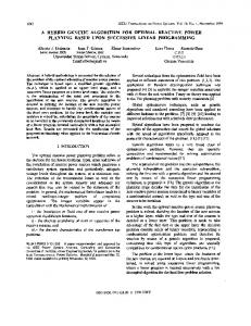
E. Hybrid Taguchi-Genetic Algorithm (HTGA) The HTGA combines the TGA with the Taguchi method. The Taguchi method is inserted between crossover and mutation operations of a TGA. Then, the systematic reasoning ability of the Taguchi method is incorporated in the crossover operations to select the better genes to achieve crossover, and consequently enhance the GA. The steps of the HTGA approach are depicted in Fig. 1 and are described as follows. Step 0) Parameter setting. • Input: population size , crossover rate , mutation rate , and number of generations. • Output: the number of function evaluations and function value. Step 1) Initial population is generated by the Algorithm given above. The function values of the population are then calculated via the test function. The times. number of function calls is calculated Step 2) Selection operation using the roulette wheel approach. Step 3) Crossover operation. The probability of crossover is determined by crossover rate . Step 4) Select a suitable two-level orthogonal array for matrix experiments. The orthogonal arrays and are used for 30 and 100 dimensions, respectively.
370
IEEE TRANSACTIONS ON EVOLUTIONARY COMPUTATION, VOL. 8, NO. 4, AUGUST 2004
Fig. 1. (Continued) HTGA for global numerical optimization problem.
Fig. 1. HTGA for global numerical optimization problem.
Choose randomly two chromosomes at a time to execute matrix experiments. Step 6) Calculate the function values and SNRs of ex. periments in the orthogonal array Step 7) Calculate the effects of the various factors ( and ). Step 8) One optimal chromosome is generated based on the results from Step 7. Step 9) Repeat Steps 5 through 8 until the expected has been met. number Step 10) The population via the Taguchi method is generated. The number of function calls is calculated
times, where comes experimental runs of an orthogonal array plus one run for the optimum chromosome generated by SNRs. Mutation operation. The probability of mutation . The expected is determined by mutation rate number of function calls is calculated times. Offspring population is generated. Sort the fitness values in increasing order among parents and offspring populations. Select the better chromosomes as parents of the next generation. Has the stopping criterion been met? If yes, the expected number of function calls is calculated from
Step 5)
Step 11)
Step 12) Step 13) Step 14) Step 15)
TSAI et al.: HYBRID TAGUCHI-GENETIC ALGORITHM FOR GLOBAL NUMERICAL OPTIMIZATION
times, where is the number of execution generation, then go to Step 16. Otherwise, return to Step 2 and continue through Step 15. Step 16) Display the number of function calls, the optimal chromosome, and the optimal fitness value. Example 3: Here, we provide an illustrative example to show how the HTGA works. The test function is chosen and would be minimized. Suppose that there are seven . dimensions (factors) and the feasible solution space is The steps of the HTGA approach are shown as follows. Step 0) Parameter setting: population size , crossover . rate , and mutation rate Step 1) Initial population is randomly generated as follows. For example
as shown in Table I The orthogonal array is chosen, because seven dimensions (factors) are . equal to seven columns of Step 5) Choose randomly two chromosomes at a time to execute matrix experiments. Suppose two chromosomes and are chosen at this experiment. Steps 6-8) The steps are similar to those of Example 2. Step 9) Repeat Steps 5 through 8 until the expected has been met. number Step 10) The population via the Taguchi method is generated. For example
Step 4)
Step 11)
Step 2)
Step 3)
371
Mutation operation. The probability of mutation is determined by mutation rate . For example, is selected for mutation, and the chromosome the two points are randomly selected at the third and fifth genes as follows:
Based on (3.3) and a random value , the resulting offspring by calculating the linear combinations at the third and fifth genes would be
Selection operation. For example
Step 12)
Offspring population is generated. For example
Crossover operation. are For example, two chromosomes and selected for crossover, and the cut-point is randomly selected at the third gene as following:
Step 13)
Sort the fitness values in increasing order among parents and offspring populations. For example
Based on (3.1) and a random value , the resulting offspring by exchanging the right parts of their parents after the third gene and calculating the linear combinations at the cut-point genes would be
Step 14)
Select the better chromosomes as parents of the next generation. Has the stopping criterion been met? If yes, then go to Step 16. Otherwise, return to Step 2 and continue through Step 15. The optimal chromosome and fitness value are
Step 15) The probability of crossover is set as , so of chromosomes we expect that, on average, undergo crossover.
Step 16)
and
372
IEEE TRANSACTIONS ON EVOLUTIONARY COMPUTATION, VOL. 8, NO. 4, AUGUST 2004
TABLE III TEST FUNCTIONS
IV. COMPUTATIONAL RESULTS AND COMPARISONS Most researchers of global numerical optimization have used the well-known test functions in Table III to test the perfor-
mances of their improved GAs [1], [3], [5], [7], [12], [14], [17], [20], [22]. From the obtained results of numerical experiments, we can see that the OGA/Q proposed by Leung and Wang [12]
TSAI et al.: HYBRID TAGUCHI-GENETIC ALGORITHM FOR GLOBAL NUMERICAL OPTIMIZATION
373
TABLE IV COMPARISONS BETWEEN HTGA AND OGA/Q UNDER THE SAME EVOLUTIONARY ENVIRONMENTS
not only can find optimal or close-to-optimal solutions but also can give more robust and significantly better results than those other improved GAs proposed by Renders and Bersini [17], Michalewicz [14], Gen and Cheng [7], Yen and Lee [22], Chellapilla [3], Wang [20], Angelov [1], and Dai et al. [5]. Therefore, in this section, we adopt the well-known test functions in Table III to test our proposed HTGA, and to compare the performances of our proposed HTGA with the performances of OGA/Q presented by Leung and Wang [12]. In this paper, we execute our proposed HTGA to solve these test functions in Table III with the following dimensions: 1) the problem dimension for and is 30 and 2) the problem dimension for is 100. In this manner, these test functions have so many local minima that they are challenging enough for performance evaluation, and the existing results reported by Leung and Wang [12] can be used for a direct comparison.
In the work of Leung and Wang [12], the following evolutionary environments are used: the population size is 200, the crossover rate is 0.1, and the mutation rate is 0.02. In addition, the execution of the OGA/Q is stopped when the smallest cost of the chromosomes cannot be further reduced in the successive 50 generations after 1000 generations. Each test function was performed in 50 independent runs and the following results were recorded: 1) the mean number of function evaluations; 2) the mean function value (i.e., the mean of the function values was found in the 50 runs); and 3) the standard deviation of the function values. In the computational experiments of our proposed HGTA, the evolutionary parameters are designed in two contrasting cases for the sake of the comparison with the OGA/Q. In the first case, the HTGA uses the same evolutionary parameters as those adopted by the OGA/Q, whereas in the second case the different sets of evolutionary parameters are used in the HTGA. Note,
374
Fig. 2.
IEEE TRANSACTIONS ON EVOLUTIONARY COMPUTATION, VOL. 8, NO. 4, AUGUST 2004
Some of convergence results of the test functions.
however, that the stopping criterion adopted in the OGA/Q is not applicable to the HTGA, because the number of generations is no more than 1000 in the HTGA, at which time the fitness member of the population of the HTGA has already reached a fitness value equal to the mean of the OGA/Q population. Therefore, we set up another stopping criterion under which the execution of the algorithm of the proposed HTGA would be stopped as soon as the smallest function value of the fitness member of
the population is less than or equal to the mean function value given by the OGA/Q. As in the work of Leung and Wang [12], each test function was performed with 50 independent runs. The mean number of function evaluations, the mean function value, and the standard deviation of the function values are all recorded for each test function. Table IV shows the performance comparisons between the proposed HTGA and the OGA/Q given by Leung and Wang
TSAI et al.: HYBRID TAGUCHI-GENETIC ALGORITHM FOR GLOBAL NUMERICAL OPTIMIZATION
375
TABLE V COMPARISONS BETWEEN HTGA AND OGA/Q UNDER DIFFERENT EVOLUTIONARY ENVIRONMENTS
[12] under the same evolutionary environments, except for the stopping criterion. For each test function, as the stopping criterion is met, the number of generations is much less than 1000. Some of the convergence results of the test functions are shown in Fig. 2. The reason why the stopping criterion is redefined can be clearly seen from Fig. 2. From Table IV, the following can be observed. • The proposed HTGA can find optimal or close-to-optimal solutions. and , the proposed HTGA • For , , , , , can give better and closer-to-optimal solutions than the and , both HTGA OGA/Q, and for , , , and OGA/Q can give the same optimal or close-to-optimal solutions. • Except for the test function , the proposed HTGA gives smaller standard deviations of function values than the OGA/Q and, hence, the proposed HTGA has a more stable solution quality.
• The proposed HTGA requires fewer mean numbers of function evaluations than the OGA/Q and, hence, the proposed HTGA has a lower computational time requirement. Furthermore, the execution of the proposed HTGA can be stopped for each run under the stopping criterion defined above, so that the standard deviation of function values for each function except is 0. For the test function , the HTGA can find a close-to-optimal solution, which is already very close to the global minimum 0, but the OGA/Q can find closer-to-optimal solution by using more function evaluations. In other words, these results in Table IV indicate that the proposed HTGA can, in general, give better mean solution quality and more stable solution quality than the OGA/Q. Now, we turn to study the second case that the different sets of evolutionary parameters are used in the HTGA. Optimizing the main parameters of the GA, namely, the population size, probability of crossover, and probability of mutation, continues to be a topic of active research even up to this day. The adaptation of the main parameters can help improve the performance of a
376
IEEE TRANSACTIONS ON EVOLUTIONARY COMPUTATION, VOL. 8, NO. 4, AUGUST 2004
GA [6], [9]. The Taguchi method can be also applied to find the optimal evolutionary parameters in the GA such that the performance of the GA can be improved [4]. Here, we divide the evolutionary parameters in the second case into two separate groups in order to achieve better performance and get smaller numbers of function calls. In the first group, the population size is 200, the crossover rate is 0.1, and the mutation rate is 0.2 for , , , , , and , whereas in the second group they are 200, 0.1, and 0.0, respectively, i.e., without using the mutation , and . The computational results and operator, for , , comparisons are shown in Table V. We can see that, by using the HTGA approach under the suitable combination of the evolutionary parameters, the mean numbers of function evaluations for all test functions in Table V are smaller than those shown in Table IV, suggesting that the optimal results can be found under the suitable combination of the evolutionary parameters and that the HTGA gives, again, better and more robust results as a whole. Here, we discuss one specific issue how and why the convergence dynamics of the HTGA are different to those of the OGA/Q. Leung and Wang [12] did not provide any graphs of convergence dynamics of the OGA/Q in their paper, so we cannot compare graphically the convergence dynamics of the HTGA with those of the OGA/Q. But, we still could provide some helpful evidences from the results in Tables IV and V to explain the convergence differences between the HTGA and the OGA/Q as follows. 1) From Tables IV and V, we can see that, as the stopping criterion is met, the HTGA requires much less mean numbers of function evaluations than the OGA/Q, that is the HTGA has faster convergence speed than the OGA/Q. 2) From Tables IV and V, we can see that the execution of the HTGA can be stopped for every run under that the stopping criterion is met, so that, except for , the standard deviation of the function values for each test function is 0. However, by using the OGA/Q method, only six test functions have the results mentioned above. Therefore, The HTGA gives better stability of convergence than the OGA/Q. 3) It can be seen from Fig. 2 that, for the most test functions, the number of convergence generations is no more than 200 by using the HTGA. However, the stopping criterion defined in the OGA/Q is that the execution is stopped when the smallest cost of the chromosomes cannot be further reduced in the successive 50 generations after 1000 generations. From the mean number of function evaluations and the standard deviation of function values as shown in Table IV by using the OGA/Q, we can infer that the number of convergence generations is more than 1000 for each test function by using the OGA/Q. Therefore, we could conclude that the HTGA gives smaller convergence generations than the OGA/Q. Besides, we here also discuss the other specific issue as follows. The OGA/Q evenly scans the feasible solution space once to locate the good points for further exploration in subsequent iterations. As the algorithm iterates itself and improves
the population of points, some points may move closer to the global optimum than the others. Those points are then used as the initial population of points for further exploration [12]. In contrast, our HTGA randomly generates an initial population instead of evenly scanning the feasible solution space to find good points as initial population. But, in this way, the proposed HTGA still can find the optimal or close-to-optimal solutions, and give better mean solution quality and more stable solution quality than the OGA/Q, so that it can be more robust and statistically sounder than the OGA/Q. V. CONCLUSION In this paper, the HTGA has been presented to solve global numerical optimization problems with continuous variables. The HTGA combines the TGA, which has the merit of powerful global exploration capability, with the Taguchi method, which can exploit the optimum offspring. The two-level orthogonal array and the SNR of the Taguchi method are used for exploitation. The optimum chromosome can be easily found by using both experimental runs and SNRs instead of executing combinations of factor levels, which are all combinations of factor levels. Moreover, the Taguchi method is also a robust design approach, which draws on many ideas from statistical experimental design to plan experiments for obtaining dependable information about variables, so it can achieve the population distribution closest to the target and make the results robust. In the proposed HTGA, the Taguchi method is inserted between crossover and mutation operations of a TGA. Then, the systematic reasoning ability of the Taguchi method is incorporated in the crossover operations to select the better genes to achieve crossover, and consequently enhance the genetic algorithm. Therefore, the proposed HTGA possesses the merits of global exploration, fast convergence, robustness, and statistical soundness. We executed the proposed HTGA to solve 15 benchmark problems with 30 or 100 dimensions, where some of these problems have numerous local minima. The computational experiments show that the proposed HTGA can find optimal or close-to-optimal solutions, and it is more efficient than the OGA/Q presented by Leung and Wang [12] on the problems studied. ACKNOWLEDGMENT The authors would like to thank the referees and Prof. X. Yao for their constructive and helpful comments and suggestions. REFERENCES [1] P. Angelov, “Supplementary crossover operator for genetic algorithms based on the center-of-gravity paradigm,” Control Cybern., vol. 30, pp. 159–176, 2001. [2] M. Bazaraa, J. Jarvis, and H. Sherali, Linear Programming and Network Flows. New York: Wiley, 1990. [3] K. Chellapilla, “Combining mutation operators in evolutionary programming,” IEEE Trans. Evol. Comput., vol. 2, pp. 91–96, Sept. 1998. [4] J. H. Chou, W. H. Liao, and J. J. Li, “Application of Taguchi-genetic method to design optimal grey-fuzzy controller of a constant turning force system,” in Proc. 15th CSME Annu. Conf., Tainan, Taiwan, 1998, pp. 31–38. [5] X. M. Dai, Z. G. Chen, R. Feng, X. F. Mao, and H. H. Shao, “Improved algorithm of pattern extraction based mutation approach to genetic algorithm,” J. Shanghai Jiaotong Univ., vol. 36, pp. 1158–1160, 2002.
TSAI et al.: HYBRID TAGUCHI-GENETIC ALGORITHM FOR GLOBAL NUMERICAL OPTIMIZATION
[6] L. Davis, “Adapting operator probabilities in genetic algorithms,” in Proc. Int. Conf. Genetic Algorithms ICGA 89, San Mateo, CA, 1989, pp. 61–69. [7] M. Gen and R. Cheng, Genetic Algorithms and Engineering Design. New York: Wiley, 1997. [8] D. E. Goldberg, Genetic Algorithms in Search, Optimization and Machine Learning. reading: Addison-Wesley, 1989, ch. MA. [9] J. J. Grefenstette, “Optimization of control parameters for genetic algorithms,” IEEE Trans. Syst. Man Cybern., vol. SMC–16, pp. 122–128, 1986. [10] C. H. Hsieh, J. H. Chou, and Y. J. Wu, “Taguchi-MHGA method for optimizing Takagi-Sugeno fuzzy gain-scheduler,” in Proc. 2000 Automatic Control Conf., Taipei, Taiwan, 2000a, pp. 523–528. , “Taguchi-MHGA method for optimizing grey-fuzzy gain-sched[11] uler,” in Proc. 6th Int. Conf. Automation Technology, Taipei, Taiwan, 2000b, pp. 575–582. [12] Y. W. Leung and Y. Wang, “An orthogonal genetic algorithm with quantization for global numerical optimization,” IEEE Trans. Evol. Comput., vol. 5, pp. 41–53, Feb. 2001. [13] D. C. Montgomery, Design and Analysis of Experiments. New York: Wiley, 1991. [14] Z. Michalewicz, Genetic Algorithms + Data Structures = Evolution Programs. Berlin, Germany: Springer-Verlag, 1996. [15] S. H. Park, Robust Design and Analysis for Quality Engineering. London, U.K.: Chapman & Hall, 1996. [16] M. S. Phadke, Quality Engineering Using Robust Design. Englewood Cliffs, NJ: Prentice-Hall, 1989. [17] J. Renders and H. Bersini, “Hybridizing genetic algorithms with hill-climbing methods for global optimization: two possible ways,” in Proc. 1st IEEE Conf. Evolutionary Computation, Orlando, FL, 1994, pp. 312–317. [18] P. J. Ross, Taguchi Techniques for Quality Engineering. New York: McGraw-Hill, 1989. [19] G. Taguchi, S. Chowdhury, and S. Taguchi, Robust Engineering. New York: McGraw-Hill, 2000. [20] L. Wang, Intelligent Optimization Algorithms With Applications. Beijing, China: Tsinghua Univ. Press, 2001. [21] Y. Wu, Taguchi Methods for Robust Design. New York: ASME, 2000. [22] J. Yen and B. Lee, “A simplex genetic algorithm hybrid,” in Proc. IEEE Int. Conf. Evolutionary Computation, Indianapolis, IN, 1997, pp. 175–180.
Jinn-Tsong Tsai received the B.S. and M.S. degrees in mechanical engineering from the National Sun Yat-Sen University, Kaohsiung, Taiwan, R.O.C., in 1986 and 1988, respectively. He is currently working toward the Ph.D. degree in engineering science and technology at the National Kaohsiung First University of Science and Technology, Kaohsiung, Taiwan, R.O.C. From July 1988 to May 1990, he was a Lecturer with the Vehicle Engineering Department, Chung Cheng Institute of Technology, Taiwan. Since July 1990, he has been a Researcher and the Chief of the Automation Control Section with the Metal Industries Research and Development Center, Taiwan. His research interests include evolutionary computation, intelligent control and systems, neural networks, and quality engineering.
377
Tung-Kuan Liu received the B.S. degree in mechanical engineering from the National Akita University, Akita, Japan, in 1992 and the M.S. and Ph.D. degrees in mechanical engineering and information science from the National Tohoku University, Sendai, Japan, in 1994 and 1997, respectively. He is currently an Assistant Professor with the Mechanical and Automation Engineering Department, National Kaohsiung First University of Science and Technology, Kaohsiung, Taiwan, R.O.C. From October 1997 to July 1999, he was a Senior Manager with the Institute of Information Industry, Taipei, Taiwan. From August 1999 to July 2002, he was also an Assistant Professor with the Department of Marketing and Distribution Management, National Kaohsiung First University of Science and Technology. His research and teaching interests include artificial intelligence, applications of multiobjective optimization genetic algorithms, and integrated manufacturing and business systems.
Jyh-Horng Chou (M’04–SM’04) received the B.S. and M.S. degrees in engineering science from the National Cheng-Kung University, Tainan, Taiwan, in 1981 and 1983, respectively, and the Ph.D. degree in mechatronic engineering from the National Sun Yat-Sen University, Kaohsiung, Taiwan, R.O.C., in 1988. He is currently a Professor and the Chairman of the Mechanical and Automation Engineering Department, National Kaohsiung First University of Science and Technology, Kaohsiung, Taiwan, R.O.C. From August 1983 to July 1986, he was a Lecturer with the Mechanical Engineering Department, National Sun Yat-Sen University. From August 1986 to July 1991, he was an Associate Professor with the Mechanical Engineering Department and the Director of the Center for Automation Technology, National Kaohsiung University of Applied Sciences, Kaohsiung, Taiwan, R.O.C. From August 1991 to July 1999, he was a Professor and the Chairman of the Mechanical Engineering Department, National Yunlin University of Science and Technology, Taiwan. He has coauthored three books and published more than 135 refereed journal papers. His research and teaching interests include intelligent systems and control, computational intelligence and methods, robust control, and quality engineering.