hydrus: model use, calibration, and validation - PC-PROGRESS

HYDRUS: MODEL USE, CALIBRATION, AND VALIDATION J. Šimůnek, M. Th. van Genuchten, M. Šejna

ABSTRACT. The HYDRUS numerical models are widely used for simulating water flow and solute transport in variably saturated soils and groundwater. Applications involve a broad range of steady-state or transient water flow, solute transport, and/or heat transfer problems. They include both short-term, one-dimensional laboratory column flow or transport simulations, as well as more complex, long-duration, multi-dimensional field studies. The HYDRUS models can be used for both direct problems when the initial and boundary conditions for all involved processes and corresponding model parameters are known, as well as inverse problems when some of the parameters need to be calibrated or estimated from observed data. The approach to model calibration and validation may vary widely depending upon the complexity of the application. Model calibration and inverse parameter estimation can be carried out using a relatively simple, gradient-based, local optimization approach based on the Marquardt-Levenberg method, which is directly implemented into the HYDRUS codes, or more complex global optimization methods, including genetic algorithms, which need to be run separately from HYDRUS. In this article, we provide a brief overview of the HYDRUS codes, discuss which HYDRUS parameters can be estimated using internally built optimization routines and which type of experimental data can be used for this, and review various calibration approaches that have been used in the literature in combination with the HYDRUS codes. Keywords. Calibration, HYDRUS-1D, HYDRUS (2D/3D), Numerical model, Optimization methods, Parameter estimation, Solute transport, Unsaturated soils, Validation, Water flow.

N

umerical models are increasingly used for predicting or analyzing water flow and contaminant transport processes in the subsurface, including the vadose zone. The objective of this article is to briefly review the history of development of the HYDRUS-1D and HYDRUS (2D/3D) software packages (Šimůnek et al., 2008b) that may be used for this purpose. We provide key citations, briefly summarize the theory behind the models, describe key parameters needed to run the codes, and discuss how these parameters can be obtained by model calibration. Note that many terms often encountered in the literature related to model calibration, verification, and validation, such as parameter uniqueness, identifiability, stability, and ill-posedness, are described in detail elsewhere (Carrera and Neuman, 1986; Šimůnek and de Vos, 1999; Šimůnek and Hopmans, 2002, among others) and will not be further discussed here. Over the years, various software packages from the broad family of HYDRUS codes (e.g., SWMS-2D, CHAIN_2D, HYDRUS-1D, HYDRUS-2D, HYDRUS

Submitted for review in September 2011 as manuscript number SW 9401; approved for publication by the Soil & Water Division of ASABE in April 2012. The authors are Jiří Šimůnek, Professor and Hydrologist, Department of Environmental Sciences, University of California, Riverside, California; Martinus Th. van Genuchten, Professor, Department of Mechanical Engineering, Federal University of Rio de Janeiro, Brazil; and Miroslav Šejna, Director, PC-Progress s.r.o., Prague, Czech Republic. Corresponding author: Jiří Šimůnek, Department of Environmental Sciences, University of California-Riverside, Riverside, CA 92521; phone: 951-8277854; e-mail: [email protected].

(2D/3D), UNSATCHEM, HP1, and CW2D) have become widely used tools for evaluating water flow and solute transport in soils and groundwater. For example, HYDRUS-1D was downloaded more than five thousand times in 2010 alone by users from around the world. The HYDRUS website lists almost one thousand peer-reviewed journal references in which the HYDRUS programs have been used. The codes themselves have been reviewed favorably several times in the literature, the latest one being a recent review by Yu and Zheng (2010). The number of HYDRUS-1D users is significantly larger than those of HYDRUS (2D/3D) since HYDRUS-1D remains in the public domain and as such can be downloaded freely from the HYDRUS website (www.hydrus2d.com), while HYDRUS (2D/3D) is distributed commercially for a nominal fee. The HYDRUS-1D software package may be used to simulate water flow and solute transport (as well as heat and carbon dioxide transport) in variably saturated media, assuming either a vertical, horizontal, or generally inclined direction. HYDRUS (2D/3D) similarly simulates water flow and solute/heat transport in two-dimensional vertical or horizontal planes, in axisymmetrical three-dimensional domains, or in fully three-dimensional variably saturated domains. Because the history of development of the HYDRUS (2D/3D) software package is documented in detail elsewhere (Šimůnek et al., 2008b), we will discuss here primarily the historical development of HYDRUS-1D (Šimůnek et al., 1998a, 2005, 2008a). HYDRUS-1D traces its roots to the early work of van Genuchten (1978, 1987) and his SUMATRA and WORM models, as well as later work by Vogel (1987) and Kool

Transactions of the ASABE Vol. 55(4): 1261-1274

© 2012 American Society of Agricultural and Biological Engineers ISSN 2151-0032

1261

and van Genuchten (1989) and their SWMI and HYDRUS models, respectively (fig. 1). While Hermitian cubic finite element numerical schemes were used in SUMATRA and linear finite elements were used in WORM and the older HYDRUS code for solution of both the water flow and solute transport equations, SWMI used finite differences to solve the flow equation. Various features of these four early models were combined first in the DOS-based SWMI_ST model (Šimůnek, 1993) and later in the Windows-based HYDRUS-1D simulator (Šimůnek et al., 1998a). Version 1 of HYDRUS-1D (Šimůnek et al., 1998a) was the first version that included both physical-nonequilibrium (dualporosity mobile-immobile water) and chemicalnonequilibrium (two-site sorption model) solute transport. After releasing versions 1 (for 16-bit Windows 3.1) and 2 (for 32-bit Windows 95), the next two major updates (versions 3 and 4) were released in 2005 and 2008. While version 3 of HYDRUS-1D included an option to consider dual-porosity water flow and solute transport, version 4 additionally included dual-permeability water flow and solute transport (Šimůnek and van Genuchten, 2008). The last two versions included additional modules applicable to more complex biogeochemical reactions than the standard HYDRUS modules. While the standard modules of HYDRUS-1D can simulate the transport of solutes that are either fully independent or involved in the sequential firstorder degradation chains, the two new modules can consider mutual interactions between multiple solutes, such as cation exchange and precipitation/dissolution. Version 3 included the UNSATCHEM module (Šimůnek et al., 1996; Suarez and Šimůnek, 1997) for simulating carbon dioxide transport as well as the multi-component transport of major ions. The UNSATCHEM major ion module was recently included also in version 2 of HYDRUS (2D/3D) (Šimůnek et al., 2011). Version 4 of HYDRUS-1D now includes not only the UNSATCHEM module but also the HP1 program (Jacques and Šimůnek, 2005), which resulted from coupling HYDRUS-1D with the biogeochemical program PHREEQC (Parkhurst and Appelo, 1999).

HYDRUS DESCRIPTION SIMULATED PROCESSES The standard modules of HYDRUS may be used to sim-

Figure 1. History of development of HYDRUS-1D and related software packages. All of the software packages released after 1996 are supported by graphical user interfaces.

1262

ulate the one-dimensional (in HYDRUS-1D) and two- or three-dimensional (in HYDRUS (2D/3D)) movement of water, heat, and multiple solutes in variably saturated media. The codes may be applied to unsaturated, partially saturated, or fully saturated homogeneous or layered media. The programs use mass-lumped linear finite element schemes to numerically solve the Richards equation for saturated-unsaturated flow. The unsaturated soil hydraulic properties can be described using van Genuchten (1980), Brooks and Corey (1964), modified van Genuchten (Vogel and Císlerová, 1988), Durner (1994), and Kosugi (1996) type analytical functions. The codes further incorporate hysteresis by assuming that drying scanning curves are scaled from the main drying curve and wetting scanning curves are scaled from the main wetting curve. The codes allow consideration of both equilibrium and nonequilibrium flow. The governing equations for nonequilibrium flow pertain to dual-porosity or dual-permeability flow regimes, in which a fraction of the liquid phase is assumed to be mobile (moving relatively rapidly) and another fraction is assumed to be immobile (moving relatively slowly or not at all) (Šimůnek et al., 2003; Šimůnek and van Genuchten, 2008). Both HYDRUS programs can be used to simulate such processes as precipitation, irrigation, infiltration, evaporation, root water uptake (transpiration), soil water storage, capillary rise, deep drainage, groundwater recharge, and lateral flow (the latter not in 1D). Both models can also evaluate surface runoff when the applied flux becomes larger than the infiltration capacity of the soil, as well as reduce evaporation and transpiration from their potential to actual values based on the prevailing conditions in the soil profile and specific properties of the vegetation. The flow equations additionally include sink terms to account for water uptake by plant roots as a function of both water and salinity stress. The codes can simulate both compensated and uncompensated root water uptake, as well as both active and passive nutrient root uptake (Jarvis, 1989; Šimůnek and Hopmans, 2009). Heat and contaminant transport processes in the HYDRUS-1D and HYDRUS (2D/3D) programs are described using Fickian-based advection-dispersion type equations, which are solved numerically using linear finite element schemes. The solute transport equations assume advective-dispersive transport in the liquid phase and diffusion in the gaseous phase. The transport equations further include provisions for nonlinear and/or nonequilibrium reactions between the solid and liquid phases, linear equilibrium reactions between the liquid and gaseous phases, zeroorder production, and two first-order degradation reactions, one that is independent of other solutes, and one that provides the coupling between solutes involved in sequential first-order decay reactions (Šimůnek et al., 2008b). In addition, physical nonequilibrium transport can be accounted for by assuming several two-region, dual-porosity type formulations that partition the liquid phase into mobile and immobile regions. Chemical nonequilibrium transport can be accounted for by dividing the sorption sites of the solid phase into sites subject to instantaneous sorption and sites with kinetic sorption (Selim et al., 1976; van Genuchten,

TRANSACTIONS OF THE ASABE

1981; van Genuchten and Wagenet, 1989; Šimůnek and van Genuchten, 2008). Because of the relatively general formulation of the transport and reaction terms, the HYDRUS codes can be used to simulate the fate and transport of many different solutes, including non-adsorbing tracers, radionuclides (e.g., Mallants et al., 2003; Pontedeiro et al., 2010), mineral nitrogen species (Hanson et al., 2006), pesticides (Pot et al., 2005; Dousset et al., 2007), chlorinated aliphatic hydrocarbons (Schaerlaekens et al., 1999; Casey and Šimůnek, 2001), hormones (Casey et al., 2003), antibiotics (Wehrhan et al., 2007), and explosives/propellants (Dontsova et al., 2006, 2009). The governing transport equations were additionally modified to allow consideration of kinetic attachment/detachment processes of solutes to the solid phase, and hence of solutes having a finite size. The attachment/detachment features have been used recently in several studies to simulate the transport of viruses (e.g., Schijven and Šimůnek, 2002) colloids (Bradford et al., 2002, 2003, 2004), bacteria (Gargiulo et al., 2007a, 2007b), and nanoparticles (Torkzaban et al., 2010). The HYDRUS codes further include modules for simulating carbon dioxide transport (only in 1D) and major ion chemistry as adopted from the UNSATCHEM programs of Šimůnek and Suarez (1994) and Šimůnek et al. (1996), respectively. Gonçalves et al. (2006) and Ramos et al. (2011) recently demonstrated the applicability of these modules to simulating multicomponent major ion transport in soil lysimeters irrigated with waters of different quality. HYDRUS-1D was used in these applications to describe field measurements of the water content, overall salinity, the concentration of individual soluble cations, as well as of the sodium adsorption ratio (SAR), electric conductivity (EC), and the exchangeable sodium percentage (ESP). To make the HYDRUS codes as attractive as possible for use by inexperienced numerical modelers, students, consulting engineers, and practitioners, much effort went into the development of flexible graphics-based user interfaces. For this purpose, the HYDRUS packages use Microsoft Windows-based graphical user interfaces (GUIs) to manage the input data required to run the programs, as well as for nodal discretization and editing, parameter allocation, problem execution, and visualization of the results. All spatially distributed parameters, such as those for delineating various soil horizons, root water uptake distributions, and the initial and boundary conditions for water, heat, and solute movement, are specified in graphical environments. The programs further include a small catalog of unsaturated soil hydraulic properties (Carsel and Parrish, 1988), as well as pedotransfer functions based on neural network analyses (Schaap et al., 2001). The HYDRUS models as such are not limited to any particular spatial or temporal scale, providing that the governing equations are formulated properly and can be used at that scale. There have been many successful applications of HYDRUS-1D at scales ranging from small laboratory soil columns to agricultural applications for soil profiles one or several meters deep (e.g., Gärdenäs et al., 2005; Hanson et al., 2006), up to soil profiles several hundred meters deep (e.g., Scanlon et al., 2003). HYDRUS (2D/3D) has been

55(4): 1261-1274

applied similarly to transport domains ranging from less than 1 m wide to transects of several tens or hundreds of meters wide, and involving both laboratory (e.g., Silliman et al., 2002) and field-scale applications (Siyal et al., 2009; Yakirevitch et al., 2010). However, we generally do not recommend HYDRUS to be used for large threedimensional (i.e., catchment size) applications. The highly nonlinear Richards equation requires relatively fine spatial discretization, especially at locations where large hydraulic gradients are expected, such as close to the soil surface where variable meteorological conditions can cause very rapid changes in the soil water contents and corresponding pressure heads. Spatial discretization of even a relatively small catchment can lead to hundreds of thousands, or even millions, of finite element nodes, which may significantly strain available computational resources. On the other hand, there are no limitations on the temporal scale, which can range from a few minutes for small-scale laboratory studies to hundreds of thousands of years for studies evaluating the effects of the past and current climate (e.g., Scanlon et al., 2003), the effects of the future climate change (Leterme and Mallants, 2011), or long-term environmental risk analyses of radioactive contaminants entering the subsurface (Pontedeiro et al., 2010). MODEL CALIBRATION AND INVERSE PARAMETER ESTIMATION Model calibration is generally defined as the process of tuning a model for a particular problem by manipulating the input parameters (e.g., soil hydraulic parameters) and initial or boundary conditions within reasonable ranges until the simulated model results closely match the observed variables (e.g., pressure heads, water contents, concentrations, various fluxes) (Šimůnek and Hopmans, 2002). The general approach in model calibration is to select an objective function to serve as a measure of the agreement between measured and modeled data, and which directly or indirectly is related to the adjustable parameters. The bestfit parameters are then obtained by minimizing this objective function. Model calibration can be achieved by trial and error or by using automated minimization or parameter estimation techniques. A model is considered successfully calibrated when it reproduces data within some subjectively acceptable level of precision (Konikow and Bredehoeft, 1992). Model calibration is often referred to also as history matching. When the ultimate goal of model calibration is not merely to calibrate a model but rather to optimize unknown parameters in that model, the process is often called parameter optimization or parameter estimation (Šimůnek and de Vos, 1999). Both HYDRUS software packages implement a Marquardt-Levenberg type parameter estimation technique (Marquardt, 1963; Šimůnek and Hopmans, 2002) for inverse estimation of soil hydraulic, solute transport, and/or heat transport parameters from measured transient or steady-state flow and/or transport data. For this purpose, the HYDRUS programs are written in such a way that almost any application that can be run in a direct mode (i.e., when all parameters and initial and boundary conditions are specified and predictions are made) can be run

1263

equally well in an inverse mode, and thus are effective for model calibration and parameter estimation applications. Because of its generality, the inverse option in HYDRUS has proven to be very popular with many users, leading to a large number of applications ranging from relatively simple laboratory experiments, such as one- and multi-step outflow experiments (e.g., Wildenschild et al., 2001) or evaporation experiments (Šimůnek et al., 1998b), to more elaborate field problems involving multiple soil horizons and chemicals (Vrugt et al., 2008; Wöhling et al., 2008). Refer to the HYDRUS website (www.pc-progress.com/en/ Default.aspx?hydrus-3d) for many specific examples. The objective function to be minimized during the parameter estimation process using one of the HYDRUS codes is written in a relatively general manner to allow simultaneous consideration of a large number of different types of measurements and information. The objective function, Φ, is defined as (Šimůnek et al., 1998a): Φ (b, q, p) =

mq

nqj

j =1

i =1

 v j  wi, j q*j (x, ti ) − q j (x, ti , b) mp

+

  wi, j  p*j (x,θi ) − p j (x,θi , b)  vj

j =1

+

n pj

2

nb

2

(1)

i =1

vˆ j b*j (x) − b j (x) 

2

j =1

where the first term on the right side represents deviations between measured and calculated space-time variables. In this first term, mq is the number of different sets of measurements, nqj is the number of measurements within a particular measurement set, qj*(x,ti) represents specific measurements at time ti for the jth measurement set at location x, qj(x,ti,b) represents the corresponding model predictions for the vector of optimized parameters b (e.g., soil hydraulic, heat transport, and/or solute transport and reaction parameters), and vj and wi,j are weights associated with a particular measurement set or point, respectively. The first term can include, for example, observed pressure heads, water contents, temperatures, and/or concentrations at different locations and/or times in the flow domain, or actual or cumulative fluxes versus time across a boundary of specified type. Resident or flux concentrations, liquid phase or total concentrations, and concentrations at a linear or logarithmic scale can all be used in the optimization depending on the application and data availability. The second term on the right side of equation 1 represents differences between independently measured and predicted soil hydraulic properties (e.g., retention, θ(h), and/or hydraulic conductivity, K(θ) or K(h), data) for different soil horizons (x), while the terms mp, npj, pj*(x,θi), pj(x,θi, b), vˆ j and wi,j have similar meanings as for the first term but are now used for the soil hydraulic properties. The last term of equation 1 represents a penalty function for deviations between prior knowledge of the soil hydraulic parameters, bj*(x), and their final estimates, bj(x), with nb being the number of parameters with prior knowledge and vj repre-

1264

senting pre-assigned weights. The Marquardt-Levenberg parameter estimation approach implemented in the HYDRUS codes assumes that the covariance (weighting) matrices, which provide information about the measurement accuracy as well as possible correlation between measurement errors and/or the parameters, are diagonal (Šimůnek and Hopmans, 2002). The weighting coefficients, vj, may be used to minimize differences in weighting between different data types because of different absolute values and numbers of data involved. They can either be specified as an input parameter or weighted proportionally to the means or variances of individual data sets. In addition, the inverse option as currently implemented in HYDRUS can be used to estimate a range of soil hydraulic parameters, heat transport parameters, and/or solute transport and reaction parameters. However, the inverse option cannot be used to estimate other variables or parameters, such as initial and boundary conditions or root water uptake parameters. In that case, other (external) optimization tools need to be used. Finally, we note that the Marquardt-Levenberg method in the HYDRUS programs is a local optimization gradient method that requires initial estimates of the unknown parameters to be optimized. The behavior of the objective function, Φ, in the neighborhood of this initial estimate is used to select a direction vector, from which updated values of the unknown parameter vector b in equation 1 are determined. Depending on the problem being considered (i.e., the magnitude of the measurement errors, the number of optimized parameters, and the type of measurements), the objective function may be topographically very complex without having a well-defined global minimum, or having several local minima in the parameter space (Šimůnek and Hopmans, 2002). The minimization can then be very sensitive to the initial values of the optimized parameters. Depending on the initial estimate, the final solution of the calibration may then not be the global minimum, but instead a local minimum. Consequently, it is generally recommended to repeat the minimization problem with different initial estimates of the optimized parameters and then select those parameter values that minimized the objective function. Alternatively, more robust global minimization techniques could be used, as will be discussed later.

ESTIMATION OF PARAMETERS USING HYDRUS SOIL HYDRAULIC PARAMETERS Variably saturated flow models, such as the HYDRUS codes, need as input the unsaturated soil hydraulic properties comprising the water retention curve (or soil moisture characteristic) and the hydraulic conductivity function. While these properties can be measured both in the laboratory and in the field, standard protocols using classical steady-state methods are generally very elaborate, timeconsuming, and hence expensive. Alternative and much faster transient methods, usually combined with numerical inversion of the flow process, have been studied extensively throughout the 1980s, 1990s, and up to the present (van

TRANSACTIONS OF THE ASABE

Genuchten et al., 1999; Hopmans et al., 2002b). Because of their inverse options, the HYDRUS codes have been used in many of these studies. HYDRUS-1D example applications include one-step and multi-step outflow experiments (Wildenschild et al., 2001; Bitterlich et al., 2004; Laloy et al., 2010; Schelle et al., 2010), evaporation experiments (Šimůnek et al., 1998b; Schindler et al., 2010), horizontal infiltration (Šimůnek et al., 2000; Jacques et al., 2012), upward infiltration (Šimůnek et al., 2001; Young et al., 2002), and centrifuge experiments (Šimůnek and Nimmo, 2005; Nakajima and Stadler, 2006; van den Berg et al., 2009), among others. HYDRUS (2D/3D) examples include experiments with tension disc permeameters (Šimůnek and van Genuchten, 1996, 1997), a modified cone penetrometer (Gribb et al., 1998; Kodešová et al., 1998; Šimůnek et al., 1999a), and a multistep soil-water extraction method (Inoue et al., 1998). The physical principles of most of these methods are discussed at length in several sections of the SSSA Methods monograph by Dane and Topp (2002). Later, we briefly discuss a case study in which the inverse option of HYDRUS is used to estimate the unsaturated soil hydraulic properties from an evaporation experiment carried out on a small laboratory soil core. All of the above studies assume equilibrium flow processes in combination with relatively standard functions for the unsaturated soil hydraulic properties. A large number of studies also exist in which parameters of various nonequilibrium flow and transport models, including especially selected dual-porosity or dual-permeability flow formulations, have been estimated using the HYDRUS codes (e.g., Pot et al., 2005; Dousset et al., 2007). Refer to Köhne et al. (2009a, 2009b) for a detailed review of these applications. We note that the HYDRUS models implement only one single overall approach to modeling preferential and nonequilibrium water flow (i.e., the flow is consistently described using the Richards equation or various modifications thereof), while many other approaches have been developed in the literature and implemented in other models (for a review of these approaches, see Šimůnek et al., 2003, including those discussed in this special collection. It is still an open question which approach is more suitable to different conditions (e.g., Köhne et al., 2009a, 2009b). SOLUTE TRANSPORT AND REACTION PARAMETERS When, in addition to water flow, solute transport is also simulated, the models need various solute transport (e.g., dispersivities, diffusion coefficients in the liquid and gaseous phases) and reaction (sorption and degradation) parameters as input. These transport and reaction parameters are often obtained using laboratory column studies that are carried out under steady-state water flow conditions. One standard laboratory procedure for obtaining some of these parameters is to carry out miscible displacement experiments in short columns and analyze the observed effluent curves using analytical solutions of the advectiondispersion equation (e.g., Skaggs et al., 2002). A large number of such analytical solutions for different initial and boundary conditions, as well as for one- and multidimensional applications, have been assembled in the STANMOD software package (Šimůnek et al., 1999b;

55(4): 1261-1274

Šimůnek et al., 2008b), which is widely used for these types of transport studies (see van Genuchten et al., 2012). Unfortunately, analytical solutions generally do not exist for nonlinear transport problems, such as for nonlinear sorption, colloid attachment with surface blocking, or when complex reaction pathways are present, in which case numerical solutions need to be employed. A large number of examples again exist in which the HYDRUS models have been used to identify solute transport and reaction parameters. A detailed review of various HYDRUS-1D applications to the analysis of nonlinear solute transport experiments, including transient flow conditions, is given by Šimůnek et al. (2002). Additional examples include the transport of interacting nitrogen species (Bolado-Rodríguez et al., 2010), pesticides (Pot et al., 2005; De Wilde et al., 2009, 2010; Cheyns et al., 2010), chlorinated aliphatic hydrocarbons (Casey and Šimůnek, 2001), hormones (Casey et al., 2003, 2004, 2005; Sangsupan et al., 2006; Fan et al., 2007), and explosives/propellants (Dontsova et al., 2006, 2009; Alavi et al., 2011). Refer to the HYDRUS website (www.pc-progress.com/en/Default.aspx?hydrus-3d) for additional examples. HEAT TRANSPORT PARAMETERS The governing equation describing heat transport in soils and other porous media contains several parameters representing the thermal properties of the medium involved. These properties include thermal volumetric capacities of individual soil constituents (e.g., solid mineral phase, organic matter), the thermal dispersivity, and the thermal conductivity function (dependent on water content). All of these parameters can be estimated from measured soil temperatures using one of the HYDRUS codes. Examples in which soil thermal parameters have been estimated using HYDRUS include studies by Hopmans et al. (2002a), Mortensen et al. (2006), Saito et al. (2007), and Sakai et al. (2009). OTHER PARAMETERS Several other model parameters, such as those describing root water uptake and root distributions (e.g., Vrugt et al., 2001a, 2001b), have also been estimated using the HYDRUS codes. However, since in general this cannot be done directly using the standard HYDRUS inverse option, either the HYDRUS source code needs to be modified or some external optimization tool must be employed. We will not here further discuss particular applications of the modified HYDRUS codes. However, in the next section, we briefly discuss external tools that have been used in combination with HYDRUS to optimize various HYDRUS model parameters and to calibrate the HYDRUS codes.

ESTIMATION OF PARAMETERS USING EXTERNAL OPTIMIZATION TOOLS MODEL-INDEPENDENT OPTIMIZATION TOOLS Two general, model-independent, parameter optimization packages that have been popularly used in subsurface hydrology are PEST (Doherty, 2005) and UCODE (Poeter

1265

et al., 2005). While initially developed for the groundwater flow model MODFLOW, both codes have since been used with other models, including HYDRUS. PEST and UCODE provide users with great flexibility in choosing which parameters to optimize and which variables to use in the objective function. As such, they can also be used with HYDRUS to optimize parameters and to use variables and information that would not have been possible with the standard HYDRUS inversion option. Still, we note that both PEST and UCODE use a gradient-type minimization method similar to the one used by the HYDRUS models and thus are equally prone to finding local rather than global minima. Example applications of the PEST program with HYDRUS are studies by Singh et al. (2010) and Singh and Wallender (2011), who evaluated soil hydraulic parameters from field data sets at different levels of soil water salinity, and by Huang et al. (2011), who analyzed infiltration and drainage processes in multi-layered coarse soils. The UCODE software was used in combination with HYDRUS-1D by Dahiya et al. (2007) to simultaneously optimize the soil hydraulic parameters of several soil layers, as well as the potential evaporation rate. Recently, Jacques et al. (2012) documented the use of UCODE to optimize soil hydraulic and solute transport parameters, as well as cation exchange capacity (CEC) and the Gapon exchange constants from observed water content, Cl concentration, and total aqueous and sorbed concentration profiles of three major cations (Ca, Mg, and K) during water absorption into a horizontal column. While the standard HYDRUS-1D inverse option was used to estimate soil hydraulic and solute transport parameters, HP1 was used to estimate CEC and the Gapon exchange constants. GENETIC ALGORITHMS Local gradient-based optimization algorithms, such as the Levenberg-Marquardt scheme (Marquardt, 1963), generally work best when only a limited number of parameters need to be identified. An alternative is needed when a larger set of parameters is involved, such as when optimizing soil hydraulic parameters for multiple horizons (Vrugt et al., 2001b). While many different global optimization algorithms, such as simulated annealing, stochastic approximation methods, evolution algorithms, multiple-level singlelinkage methods, interval arithmetic techniques, taboo search schemes, subenergy tunneling, and non-Lopschitzian terminal repellers, have been developed in the past (e.g., see references in Oreskes et al., 1994; Barhen et al., 1997), only a few of these have been used in combination with the HYDRUS models. Genetic algorithms provide a powerful tool for parameter identification when the number of fitting parameters is large (Bäck, 1996). Genetic algorithms were developed in evolution theory based on the concepts of natural selection and genetics. Vrugt et al. (2001a, 2001b) used a genetic algorithm to simultaneously identify soil hydraulic, root water uptake, and root distribution parameters, which would be very difficult, if not impossible, with the standard parameter approaches implemented in HYDRUS. Although

1266

genetic algorithms are effective in determining the general region with the global minimum (if it exists), they are not necessarily the most efficient in finding the exact optimum location. For this reason, Vrugt et al. (2001a) only used a genetic algorithm to identify the region where the global minimum of the objective function existed, and then used the results of the genetic algorithm as initial values in a simplex optimization to determine the local minimum within the global minimum region. Zhang et al. (2010) similarly used genetic algorithms to infer the effective soil hydraulic properties from field evaporation experiments. SCEM-UA, AMALGAM, AND OTHER GLOBAL OPTIMIZATION TOOLS The SCEM-UA (Shuffled Complex Evolution MetropolisUniversity of Amsterdam/Arizona) algorithm (Vrugt et al., 2003b), which is based on the Markov chain Monte Carlo (MCMC) method, is likely the most commonly used external global optimization method employed with HYDRUS. This method was successfully used to identify soil hydraulic parameters using HYDRUS by Vrugt et al. (2003a, 2004), Schoups et al. (2005), and Mertens et al. (2006), among many others. The number of global optimization tools that are being developed is still increasing rapidly. For example, Wöhling et al. (2008) used HYDRUS to estimate the soil hydraulic parameters of multiple soil horizons using three global optimization algorithms: the Nondominated Sorting Genetic Algorithm (NSGA-II), the Multi-objective Shuffled Complex Evolution Metropolis algorithm (MOSCEM-UA), and AMALGAM, the latter being A Multi-ALgorithm Genetically Adaptive search Method for multi-objective estimation of soil hydraulic parameters. A recent review of many new developments, including the use of methods suitable for massively parallel computing, is given by Vrugt et al. (2008).

DISCUSSION MODEL PARAMETERS AND CALIBRATION The HYDRUS codes are physically based models and as such require little or no calibration when all required input parameters (i.e., soil hydraulic parameters for water flow, solute transport and reaction parameters for solute transport, and thermal parameters for heat transport) are experimentally determined. Several examples can be found in the literature where the HYDRUS models have been successfully applied to laboratory and field experiments using parameters that were all determined independently of the modeling itself and hence were not calibrated. Very comprehensive studies, in which all required input parameters were determined independently, were carried out by Gonçalves et al. (2006) and Ramos et al. (2011). They determined soil hydraulic and solute transport parameters on laboratory columns and reaction parameters (Gapon selectivity coefficients) from chemical analysis, and then used HYDRUS to successfully simulate water contents, solute concentrations of individual cations, and various integral variables (such as SAR, EC, and ESP) in multiple lysime-

TRANSACTIONS OF THE ASABE

ters irrigated with waters of different qualities. However, these were relatively unique studies where much effort went into accurate measurement of all parameters. In most applications, one or more parameters required by the model may be missing. HYDRUS offers several options for determining the missing parameters for such conditions, with calibration being only one option. For example, when users do not have estimates of the soil hydraulic parameters, they can either use a catalog of average parameters for 12 textural classes of the USDA textural triangle (Carsel and Parrish, 1988) or pedotransfer functions as derived by Schaap et al. (2001) using their Rosetta program. Rosetta is a widely used computer program for estimating soil hydraulic parameters from soil textural properties using hierarchical pedotransfer functions. HYDRUS additionally includes a small database with parameters of the water stress response functions that reduce the potential root water uptake rate as a result of water and salinity stress. When transient laboratory or field data exist, these can be used in combination with Rosetta-type pedotransfer functions or other information, including independently determined flow and transport parameters, to calibrate the HYDRUS models. The pedotransfer-derived or independently determined parameters can be then used as initial estimates in the model calibration, or as prior information in the Bayesian sense such that the model can penalize for any deviations from this prior information (e.g., Šimůnek and Hopmans, 2002). In addition to the final values of the optimized parameters, the parameter estimation modules in HYDRUS also report estimates of the 95% confidence intervals, as well as mutual correlations between the parameters (see Šimůnek and Hopmans, 2002). Any type of uncertainty, such as in the measured data, the specified initial and boundary conditions, or the overall conceptual model, has an adverse effect and will be reflected in these two statistical measures. Both the confidence intervals for optimized parameters and their mutual correlations increase with input uncertainties. However, because of the nonlinearity of the overall flow problem, it is impossible to make exact predictions about how uncertainty in the input would propagate into modeling output or uncertainty in the calibrated parameters without a detailed analysis of the particular problem being investigated. Both statistical measures can be obtained from analyses of the objective function in the vicinity of the final optimized values. Both indicate how well the optimized parameters are estimated, or if they can be optimized at all. Strong correlations between the optimized parameters indicate that the parameters cannot be simultaneously optimized and that one of the parameters should be independently determined and fixed during the optimization process. Alternatively, perhaps additional data could be included in the objective function to diminish correlation. Hence, the correlation matrix may be used to identify nonadjustable parameters because of their high correlation with other fitting parameters. Interdependence of the optimized parameters often also causes slow convergence and non-uniqueness during the inversion process and increased parameter uncertainty.

55(4): 1261-1274

For highly nonlinear problems, such as many variably saturated flow studies, it is sometimes difficult to estimate a priori what information to collect and which parameters to optimize in order to obtain a well-posed parameter estimation solution. It is not always immediately obvious whether or not a given type of experiment, or a given data set, will result in a well-posed inverse problem, or how many parameters can be uniquely estimated. Since it is not always clear what may cause a non-unique or unstable solution, inverse problems always require an in-depth analysis to determine whether or not the problem is well-posed and, if not, what causes the ill-posedness (Šimůnek and van Genuchten, 1996; Šimůnek and Hopmans, 2002). While the HYDRUS codes have been used in several studies to identify soil hydraulic parameters for multiple soil horizons (e.g., Jacques et al., 2002; Dahiya et al., 2007; Wöhling et al., 2008; Huang et al., 2011), an important question remains: whether the models can also be used to estimate effective soil hydraulic properties for the entire soil profile, assuming its homogeneity (e.g., Jacques et al., 2002; Durner et al., 2008; Schelle et al., 2012). For example, in attempts to estimate effective soil hydraulic properties of lysimeters with layered soils, Durner et al. (2008) found that although boundary fluxes of the lysimeters could be matched closely using effective properties, internal states could not be described correctly. Furthermore, the effective properties depended on the boundary conditions and the sequence of soil layers, and hence no unique effective properties could be found. Similar conclusions about the non-uniqueness of effective soil hydraulic properties and their dependence on boundary conditions were obtained in studies by Zhu and Mohanty (2002), Mohanty and Zhu (2007), Vereecken et al. (2006), and Zhu et al. (2007), among others. HISTORICAL VALIDATION If one accepts the notion that models can be formally validated (e.g., see the discussions by Konikow and Bredehoeft, 1992, and Oreskes et al., 1994, among others), the optimized model parameters are often validated using a two-step calibration scheme or split sampling. The existing data set is then divided into two parts, with the first (calibration) part being used to calibrate the model and to estimate all necessary parameters, while the second (validation or verification) part of the data set serves to compare predicted and measured data using the parameters found during the calibration (Šimůnek and de Vos, 1999). Although successful performance of the model during the second part does not constitute a rigorous validation of the model, it is often accepted that the model is validated if it predicts the system response during this second phase within acceptable limits (Anderson and Woessner, 1991). A two-step calibration process of this type is sometimes called historical validation. Many examples exist of historical validation of the HYDRUS codes with parameters estimated using model calibration. An early example is given by Šimůnek and de Vos (1999), while more recent applications are provided by Luo and Sophocleous (2010), Wang et al. (2010), and Zhao et al. (2010), among others.

1267

CASE STUDY: INVERSE ANALYSIS OF AN EVAPORATION EXPERIMENT A large number of references are given in this article of selected HYDRUS applications to a range of laboratory and field-scale studies. Hundreds of additional examples can be found on the HYDRUS website (www.pc-progress.com/en/ Default.aspx?h1d-references). In particular, we would like to direct readers to a recent study by Wöhling et al. (2008) showing a detailed analysis of flow data from a complex multilayered soil system using HYDRUS-1D in combination with three different multi-objective optimization algorithms. Here we briefly summarize a more modest application, in which the parameter estimation option of HYDRUS-1D was used to analyze data involving a laboratory evaporation experiment carried out by Wendroth et al. (1993). The example is actually one of the test cases directly distributed with the HYDRUS-1D installation files. This example shows how the parameter estimation method can be used to extract the most information from an evaporation experiment. The method, also known as Wind’s method (Wind, 1968; Arya, 2002), involves evaporation from the top of an initially saturated soil core, which is closed at the bottom, while water loss from the column is being monitored as a function of time by repeatedly weighing the core. Measurements are simultaneously made of the pressure head using tensiometers inserted at two or more depths in the column. At the end of the experiments, the sample is over-dried and average transient water contents of the core during the experiment are back-calculated by adding incremental evaporative losses between successive measurements to the final mean water content. The evaporation rate, mean water content, and tensiometer data provide the necessary information to obtain estimates of the water retention and hydraulic conductivity functions using the standard Wind method or various modifications and extensions thereof (Wendroth et al., 1993; Arya, 2002). The data for our example were obtained using an undisturbed soil core having a height of 10 cm and inside diameter of 10 cm (Wendroth et al., 1993; Šimůnek et al., 1998b). The soil had a bulk density of 1.59 g cm-3 and sand, silt, and clay fractions of 7.4%, 79.3%, and 13.3%, respectively. Five tensiometers with ceramic cups having a length of 6 cm and outside diameter of 0.6 cm were inserted horizontally through drill holes into the soil core at locations 1, 3, 5, 7, and 9 cm below the surface. An initial pressure head of -15.4 cm was measured in the middle of the soil sample. Before starting the evaporation experiment, several tension infiltrometer experiments were also carried out on the core to estimate the hydraulic conductivity at pressure heads of -1, -5, and -10 cm. Evaporation losses versus time during the experiments were obtained by weighing the core immediately after taking the tensiometer readings. The evaporation rate at the beginning of the experiments was artificially increased to approximately 1.2 cm d-1 by using a fan to blow air away from the soil surface at room temperature (Wendroth et al., 1993). Once the gradient between the tensiometers reached a value between 1.5 and 2.5 m m-1, the top of the soil sample was covered to prevent further evaporation. After re-

1268

establishing hydraulic equilibrium in the samples, evaporation was allowed to proceed without the fan at a rate of approximately 0.2 cm d-1. Measurements were taken every 30 min during the initial high-evaporation rate period and every 4 h during the second stage of evaporation. The experiment was terminated when the upper tensiometer recorded a pressure head value of -650 cm. Evaporation losses between consecutive measurements were used to define the upper flow boundary condition for the numerical simulations. This laboratory experiment was first analyzed using the modified Wind method, as described in detail by Wendroth et al. (1993). The soil hydraulic parameters were obtained by simultaneously fitting the van Genuchten (1980) soil hydraulic parameters to all of the 179 measured θ(h) and 94 K(h) data pairs, augmented with the three independently measured tension infiltrometer K(h) data points. The fitting was accomplished using the RETC code of van Genuchten et al. (1991). The hydraulic parameters consisted of the residual (θr) and saturated (θr) water contents, the van Genuchten shape factors (α and n), and the saturated hydraulic conductivity (Ks). The RETC fitted parameters are listed in table 1. Data obtained using Wind’s method and the fitted soil hydraulic functions (the thick solid lines) are shown in figure 2. The soil hydraulic parameters were also estimated from the evaporation experiment using the parameter inversion option of HYDRUS-1D. Parameter estimation was accomplished using only the first term of equation 1, in which bj = {θr, θs, α, n, Ks} represented the vector of unknown soil hydraulic parameters, while the vector qj*(x,ti) consisted of pressure heads measured at either one or several tensiometer locations (x), as well as the total amount of water in the soil core measured at the end of the experiment. The weighing coefficients wi,j in equation 1 were all fixed at 1, thus assuming that variances of the errors in the tensiometer readings were all the same. Furthermore, the weighting coefficients vj were fixed at (Šimůnek and Hopmans, 2002): vj =

1 nqj σ 2qj

(2)

which implies that the objective function Φ in this example is essentially the average weighted squared deviation between the measured and fitted values normalized by the measurement variances (σ2). Since the final water volume is only one number and the variance cannot be defined, the weight of that extra data point was also fixed at 1. Table 1 lists the optimized soil hydraulic parameters, toTable 1. Soil hydraulic parameters obtained from an evaporation experiment using parameter estimation and Wind’s method. Ks Method of α θs (cm-1) n R2 Analysis θr (cm d-1) Parameter 0.013 0.327 0.0273 1.22 88.6 0.9987 estimation (0-0.03)[a] (0.311- (0.026- (1.20- (73.20.343) 0.029) 1.24) 104.) Wind’s 0.0045 0.321 0.0249 1.23 73.3 0.992 method [a] Values in parentheses indicate 95% confidence intervals of the optimized parameters.

TRANSACTIONS OF THE ASABE

0.35

0

a)

a)

0.3

0.25

Pressure Head [cm]

Water Content [-]

-100

All tensiometers Tensiometer 1 Tensiometer 2 Tensiometer 3 Tensiometer 4 Tensiometer 5 Fitted W ind's Points W ind Method

0.2

-200 -300

Measured 1 Fitted 1 Measured 2 Fitted 2 Measured 3 Fitted 3 Measured 4 Fitted 4 Measured 5 Fitted 5

-400 -500 -600

0.15 0.5

1.0

1.5

2.0

2.5

3.0

-700

log h [cm]

0

2

0.5

1

1.5

2

b) 1

3

3.5

4

4.5

-900

-700

All Tensiometers Tensiometer 1 Tensiometer 2 Tensiometer 3 Tensiometer 4 Tensiometer 5 Fitted W ind's Points W ind Method Tension Disc Infiltration

-1 -2 -3 -4 0.0

0.5

1.0

1.5

log h [cm]

2.0

2.5

3.0

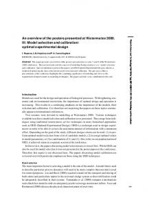
Figure 2. (a) Water retention and (b) hydraulic conductivity functions determined with inverse parameter estimation and Wind’s method. 2

gether with R values of the regressions between the predicted and measured values, as obtained by numerical inversion and Wind’s method. Figure 2 further compares plots of the resulting soil water retention and hydraulic conductivity functions. Notice the excellent agreement between the water retention curves obtained by parameter optimization and the θ(h) data points determined with Wind’s method, or their complete analytical descriptions using RETC (fig. 2a). The soil-water retention functions obtained with Wind’s method and via parameter optimization were almost identical and indistinguishable from each other (fig. 2a). The estimated unsaturated hydraulic conductivity functions obtained with the two methods (fig. 2b) were similarly very close. Figure 2 also shows results of inversions when the objective function was alternatively defined in terms of data obtained with only one tensiometer. Results remained relatively close to those obtained when readings from all tensiometers were used simultaneously. All optimizations gave similar results for the soil hydraulic properties within the range of measured pressure heads (-20 to -700 cm). Extrapolation beyond this range involved considerable uncertainty because of high correlation between the parameters θr and n. This uncertainty could be greatly reduced by including an independently measured water content at or below the wilting point in the objective function (Šimůnek et al., 1998b). Measured and fitted tensiometer readings within the soil core are shown in figure 3. The largest deviations were about 5 and 20 cm for the first (high) and second (low) evaporation rates, respectively, with most deviations being

55(4): 1261-1274

b)

t = 0.043 d t = 0.334 d t = 1.674 d t = 2.667 d t = 3.507 d t = 4.167 d Measured

-800

0

Pressure Head [cm]

log K [cm/d]

2.5

Time [d]

-600 -500 -400 -300 -200 -100 0 -10

-8

-6

z [cm]

-4

-2

0

Figure 3. Measured and fitted tensiometer readings as a function of (a) time and (b) depth.

much lower. The analyses in this example were carried out without accounting for the effects of hysteresis, which could have slightly affected the results during redistribution. In addition to the parameter estimation analysis briefly described above, Šimůnek et al. (1998b) carried out detailed analyses of the evaporation method in terms of the identifiability of various soil hydraulic parameters. A sensitivity analysis and a response surface analysis using numerically generated data showed that the optimization method was most sensitive to the soil hydraulic parameters n and θs, and least to θr. Pressure heads measured close to the soil surface were found to be more valuable for the parameter estimation analysis than those measured at lower locations, mostly because of the wider resolution of tensiometer readings near the surface. One other important conclusion was that, for the invoked experimental setup (five tensiometers in a 20 cm long core), one tensiometer reading (especially if obtained from the upper part of the core) would have been sufficient to obtain accurate estimates of the soil hydraulic functions within the range of measurements. Refer to Šimůnek et al. (1998b) for additional details about the experiments and parameter optimization analysis, and especially about the sensitivity and response surface analyses.

1269

FUTURE DEVELOPMENTS As reflected by the many references listed in this article and listed on the HYDRUS website, the HYDRUS software packages have been used over the years for a large number of applications. Feedback from users has been extremely important in identifying particular strengths and weaknesses of the codes, and for defining additional processes or features that should be included in the models. Feedback is also continuously obtained from several discussion forums at the HYDRUS website, where users can submit questions or suggestions about the models. The website also provides tutorials of the HYDRUS codes, including downloadable videos, in which the tutorials are performed step by step, thus allowing software users to teach themselves interactively. All of this is generating valuable feedback that is continuously being used to improve the codes. It is also motivating the recent and planned inclusion of additional features, such as virus and bacteria transport, more elaborate biogeochemical processes, computationally more effective approaches for coupling of vadose zone processes with existing larger-scale groundwater flow models, and overland flow. More sophisticated GUIs are also continuously being implemented, especially for the multi-dimensional codes, in an attempt to make the codes as attractive as possible for non-expert users. As such, we believe that the codes and associated manuals and tutorials are serving an important role in the transfer of vadose zone R&D technologies to both the scientific community and practitioners. The above comments also pertain to the calibration and parameter estimation capabilities of the codes. For the majority of laboratory experiments involving variably saturated water flow and transport of various solutes or particles in homogeneous soil columns, the minimization approach implemented in the HYDRUS codes seems to be sufficient at present. For such conditions, the Marquardt-Levenberg method has many significant advantages over global minimization techniques. Its main advantage is computational efficiency because the Marquardt-Levenberg approach requires far fewer evaluations of the direct model compared to global minimization techniques (tens, compared to tens of thousands), thus providing results relatively quickly (for one-dimensional problems generally within a few seconds). The iterative inverse approach is also fully automated, while global searches still often require direct involvement of users. Additionally, the Marquardt-Levenberg method provides confidence intervals for, and correlations between, the optimized parameters, thus facilitating immediate insight into the optimization problem. A major disadvantage of the Marquardt-Levenberg method is that the method searches only for a local minimum of the objective function. This will be an issue for some field-scale problems when, for example, multiple soil horizons or uncertain initial and boundary conditions are involved. The objective function may then be spatially very complex and have many local minima. Gradient-based minimization approaches, such as the Marquardt-Levenberg method, may well fail to locate the global minimum for such conditions, thus requiring the use of a global minimi-

1270

zation approach. For this reason, we are also planning to implement in HYDRUS some of the global minimization approaches, such as the MOSCEM-UA and/or AMALGAM methods, as reported by Vrugt et al. (2008), while at the same time attempting to reduce computational demands by taking advantage of the multicore structure of recent desktop processors and parallelizing the minimization problem.

REFERENCES Alavi, G., M. Chung, J. Lichwa, M. D’Alessio, and C. Ray. 2011. The fate and transport of RDX, HMX, TNT, and DNT in the volcanic soils of Hawaii: A laboratory and modeling study. J. Hazard. Mater. 185(2-3): 1600-1604. Anderson, M. P., and W. W. Woessner, 1991. Applied Groundwater Modeling: Simulation of Flow and Advective Transport. San Diego, Cal.: Academic Press. Arya, L. M. 2002. Chapter 3.6.1.1.c: Wind and hot-air methods. In Methods of Soil Analysis: Part 4. Physical Methods, 916-926. J. H. Dane and G. C. Topp, eds. SSSA Book Series 5. Madison, Wisc.: SSSA. Bäck, T. 1996. Evolutionary Algorithms in Theory and Practice: Evolution Strategies, Evolutionary Programming, Genetic Algorithms. New York, N.Y.: Oxford University Press. Barhen, J., V. Protopopescu, and D. Reister. 1997. TRUST: A deterministic algorithm for global optimization. Science 276(5315): 1094-1097. Bitterlich, S., W. Durner, S. C. Iden, and P. Knabner. 2004. Inverse estimation of the unsaturated soil hydraulic properties from column outflow experiments using free-form parameterizations. Vadose Zone J. 3(3): 971-981. Bolado-Rodríguez, S., D. García-Sinovas, and J. Álvarez-Benedí. 2010. Application of pig slurry to soils: Effect of air stripping treatment on nitrogen and TOC leaching. J. Environ. Mgmt. 91(12): 2594-2598. Bradford, S. A., S. R. Yates, M. Bettehar, and J. Šimůnek. 2002. Physical factors affecting the transport and fate of colloids in saturated porous media. Water Resour. Res. 38(12): 63.1-63.12, doi: 10.1029/2002WR001340. Bradford, S. A., J. Šimůnek, M. Bettehar, M. Th. van Genuchten, and S. R. Yates. 2003. Modeling colloid attachment, straining, and exclusion in saturated porous media. Environ. Sci. Tech. 37(10): 2242-2250. Bradford, S. A., M. Bettehar, J. Šimůnek, and M. Th. van Genuchten. 2004. Straining and attachment of colloids in physically heterogeneous porous media. Vadose Zone J. 3(2): 384-394. Brooks, R. H., and A. T. Corey. 1964. Hydraulic properties of porous media. Hydrology Paper No. 3. Fort Collins, Colo.: Colorado State University. Carrera, J., and S. P. Neuman. 1986. Estimation of aquifer parameters under transient and steady-state conditions: 2. Uniqueness, stability, and solution algorithms. Water Resour. Res. 22(2): 211-227. Carsel, R. F., and R. S. Parrish. 1988. Developing joint probability distributions of soil water retention characteristics. Water Resour. Res. 24(5): 755-769. Casey, F. X. M., and J. Šimůnek. 2001. Inverse analyses of the transport of chlorinated hydrocarbons subject to sequential transformation reactions. J. Environ. Qual. 30(4): 1354-1360. Casey, F. X. M., G. L. Larsen, H. Hakk, and J Šimůnek. 2003. Fate and transport of 17β-estradiol in soil-water systems. Environ. Sci. Tech. 37(11): 2400-2409. Casey, F. X. M., G. L. Larsen, H. Hakk, and J. Šimůnek. 2004. Fate and transport of testosterone in agriculturally significant

TRANSACTIONS OF THE ASABE

soils. Environ. Sci. Tech. 38(3): 790-798. Casey, F. X. M., J. Šimůnek, J. Lee, G. L. Larsen, and H. Hakk. 2005. Sorption, mobility, and transformation of estrogenic hormones in natural soil. J. Environ. Qual. 34(4): 1372-1379. Cheyns, K., J. Mertens, J. Diels, E. Smolders, and D. Springael. 2010. Monod kinetics rather than a first-order degradation model explains atrazine fate in soil mini-columns: Implications for pesticide fate modeling. Environ. Pollution 158(5): 14051411. Dahiya, R., J. Ingwersen, and T. Streck. 2007. The effect of mulching and tillage on the water and temperature regimes of a loess soil: Experimental findings and modeling. Soil and Tillage Res. 96(1): 52-63. Dane, J. H., and G. C. Topp, eds. 2002. Methods of Soil Analysis: Part 4. Physical Methods. SSSA Book Series 5. Madison, Wisc.: SSSA. De Wilde, T., J. Mertens, J. Šimůnek, K. Sniegowksi, J. Ryckeboer, P. Jaeken, D. Springael, and P. Spanoghe. 2009. Characterizing pesticide sorption and degradation in microscale biopurification systems using column displacement experiments. Environ. Pollution 157(2): 463-473. De Wilde, T., P. Spanoghe, K. Sniegowksi, J. Ryckeboer, P. Jaeken, and D. Springael. 2010. Transport and degradation of metalaxyl and isoproturon in biopurification columns inoculated with pesticide-primed material. Chemosphere 78(1): 56-60. Doherty, J. 2005. PEST: Model-Independent Parameter Estimation, User Manual. 5th ed. Brisbane, Australia: Watermark Numerical Computing. Dontsova, K. M., S. L. Yost, J. Šimůnek, J. C. Pennington, and C. Williford. 2006. Dissolution and transport of TNT, RDX, and composition B in saturated soil columns. J. Environ. Qual. 35(6): 2043-2054. Dontsova, K. M., J. C. Pennington, C. Hayes, J. Šimůnek, and C. W. Williford. 2009. Dissolution and transport of 2,4-DNT and 2,6-DNT from M1 propellant. Chemosphere 77(4): 597-603. Dousset, S., M. Thevenot, V. Pot, J. Šimůnek, and F. Andreux. 2007. Evaluating equilibrium and non-equilibrium transport of bromide and isoproturon in disturbed and undisturbed soil columns. J. Contam. Hydrol. 94(3-4): 261-276. Durner, W. 1994. Hydraulic conductivity estimation for soils with heterogeneous pore structure. Water Resour. Res. 32(9): 211223. Durner, W., U. Jansen, and S. C. Iden. 2008. Effective hydraulic properties of layered soils at the lysimeter scale determined by inverse modelling. European J. Soil Sci. 59(1): 114-124. Fan, Z., F. X. M. Casey, H. Hakk, and G. L. Larsen. 2007. Discerning and modeling the fate and transport of testosterone in undisturbed soil. J. Environ. Qual. 36(3): 864-873. Gärdenäs, A., J. W. Hopmans, B. R. Hanson, and J. Šimůnek. 2005. Two-dimensional modeling of nitrate leaching for various fertigation scenarios under micro-irrigation. Agric. Water Mgmt. 74(3): 219-242. Gargiulo, G., S. A. Bradford, J. Šimůnek, P. Ustohal, H. Vereecken, and E. Klumpp. 2007a. Transport and deposition of metabolically active and stationary phase Deinococcus radiodurans in unsaturated porous media. Environ. Sci. and Tech. 41(4): 1265-1271. Gargiulo, G., S. A. Bradford, J. Šimůnek, P. Ustohal, H. Vereecken, and E. Klumpp. 2007b. Bacteria transport and deposition under unsaturated conditions: The role of the matrix grain size and the bacteria surface protein. J. Contam. Hydrol. 92(3-4): 255-273. Gonçalves, M. C., J. Šimůnek, T. B. Ramos, J. C. Martins, M. J. Neves, and F. P. Pires. 2006. Multicomponent solute transport in soil lysimeters irrigated with waters of different quality.

55(4): 1261-1274

Water Resour. Res. 42: W08401, doi: 10.1029/2006WR004802. Gribb, M. M., J. Šimůnek, and M. F. Leonard. 1998. Development of a cone penetrometer method to determine soil hydraulic properties. ASCE J. Geotech. and Geoenviron. Eng. 124(9): 820829. Hanson, B. R., J. Šimůnek, and J. W. Hopmans. 2006. Evaluation of urea-ammonium-nitrate fertigation with drip irrigation using numerical modeling. Agric. Water Mgmt. 86(1-2): 102-113. Hopmans, J. W., J. Šimůnek, and K. L. Bristow. 2002a. Indirect estimation of soil thermal properties and water flux from heat pulse measurements: Geometry and dispersion effects. Water Resources Res. 38(1): 7.1-7.14, doi: 10.1029/2000WR000071. Hopmans, J. W., J. Šimůnek, N. Romano, and W. Durner. 2002b. Chapter 3.6.2: Inverse modeling of transient water flow. In Methods of Soil Analysis: Part 1. Physical Methods, 963-1008. J. H. Dane and G. C. Topp, eds. 3rd ed. Madison, Wisc.: SSSA. Huang, M., S. L. Barbour, A. Eishorbagy, J. D. Zettl, and B. C. Si. 2011. Infiltration and drainage processes in multi-layered coarse soils. Canadian J. Soil Sci. 91(2): 169-183. Inoue, M., J. Šimůnek, J. W. Hopmans, and V. Clausnitzer. 1998. In situ estimation of soil hydraulic functions using a multi-step soil water extraction technique. Water Resour. Res. 34(5): 1035-1050. Jacques, D., and J. Šimůnek. 2005. User Manual of the Multicomponent Variably Saturated Flow and Transport Model HP1: Description, Verification, and Examples. Version 1.0. Open report SCK•CEN-BLG-998. Mol, Belgium: SCK•CEN, Waste and Disposal Department. Available at: www.pc-progress.com/Documents/hp1.pdf. Jacques, D., J. Šimůnek, A. Timmerman, and J. Feyen. 2002. Calibration of Richards and convection-dispersion equations to field-scale water flow and solute transport under rainfall conditions. J. Hydrol. 259(1-4): 15-31. Jacques, D., C. Smith, J. Šimůnek, and D. Smiles. 2012. Inverse optimization of hydraulic, solute transport, and cation exchange parameters using HP1 and UCODE: Absorption of artificial piggery effluent by soils. J. Contam. Hydrol. (in press), doi:10.1016/j.jconhyd.2012.03.008. Jarvis, N. J. 1989. A simple empirical model of root water uptake. J. Hydrol. 107(1-4): 57-72. Kodešová, R., M. M. Gribb, and J. Šimůnek. 1998. Estimating soil hydraulic properties from transient cone permeameter data. Soil Sci. 163(6): 436-453. Köhne, J. M., S. Köhne, and J. Šimůnek. 2009a. A review of model applications for structured soils: a) Water flow and tracer transport. J. Contam. Hydrol. 104(1-4): 4-35. Köhne, J. M., S. Köhne, and J. Šimůnek. 2009b. A review of model applications for structured soils: b) Pesticide transport. J. Contam. Hydrol. 104(1-4): 36-60. Konikow, L. F., and J. D. Bredehoeft. 1992. Ground-water models cannot be validated. Advances in Water Resources 15(1): 7583. Kool, J. B., and M. Th. van Genuchten. 1991. HYDRUS: Onedimensional variably saturated flow and transport model, including hysteresis and root water uptake. Version 3.3. Research Report No. 124. Riverside, Cal.: USDA-ARS U.S. Salinity Laboratory. Kosugi K. 1996. Lognormal distribution model for unsaturated soil hydraulic properties. Water Resour. Res. 32(9): 2697-2703. Laloy, E., M. Weynants, Bielders, M. Vanclooster, and M. Javaux. 2010. How efficient are one-dimensional models to reproduce the hydrodynamic behavior of structured soils subjected to multi-step outflow experiments? J. Hydrol. 393(1-2): 37-52. Leterme, B., and D. Mallants. 2011. Climate and land use change impacts on groundwater recharge. In Proc. ModelCARE2011: Models - Repositories of Knowledge. Wallingford, U.K.: IAHS Press.

1271

Luo, Y., and M. Sophocleous. 2010. Seasonal groundwater contribution to crop-water use assessed with lysimeter observations and model simulations. J. Hydrol. 389(3-4): 325335. Mallants, D., D. Jacques, and T. Zeevaert. 2003. Modeling 226Ra, 222 Rn, and 210Pb migration in a proposed surface repository of very low-level long-lived radioactive waste. Paper No. ICEM03-4632. In Proc. ICEM2003: 9th Intl. Conf. on Radioactive Waste Mgmt. and Environ. Remediation, 823-830. New York, N.Y.: ASME. Marquardt, D. W. 1963. An algorithm for least-squares estimation of nonlinear parameters. SIAM J. Appl. Math. 11(2): 431-441. Mertens, J., R. Stenger, and G. F. Barkle. 2006. Multiobjective inverse modeling for soil parameter estimation and model verification. Vadose Zone J. 5(3): 917-933. Mohanty, B. P., and J. Zhu. 2007. Effective hydraulic parameters in horizontally and vertically heterogeneous soils for steadystate land-atmosphere interaction. J. Hydrometeorol. 8(4): 715729. Mortensen, A, P., J. W. Hopmans, Y. Mori, and J. Šimůnek. 2006. Multi-functional heat pulse probe measurements of coupled vadose zone flow and transport. Advances in Water Resources 29(2): 250-267. Nakajima, H., and A. T. Stadler. 2006. Centrifuge modeling of one-step outflow tests for unsaturated parameter estimations. Hydrol. Earth Syst. Sci. 10(5): 715-729. Oreskes, N., K. Shrader-Frechette, and K. Belitz. 1994. Verification, validation, and confirmation of numerical models in the earth sciences. Science 263(5147): 641-646. Parkhurst, D. L., and C. A. J. Appelo. 1999. User’s guide to PHREEQC (Version 2): A computer program for speciation, batch-reaction, one-dimensional transport, and inverse geochemical calculations. USGS Water Resources Investigation Report 99-4259. Reston, Va.: U.S. Geological Survey. Poeter, E. P., M. C. Hill, E. R. Banta, S. Mehl, and C. Steen. 2005. UCODE_2005 and six other computer codes for universal sensitivity analysis, calibration, and uncertainty evaluation. USGS Techniques and Methods 6-A11. Reston, Va.: U.S. Geological Survey. Pontedeiro, E. M., M. Th. van Genuchten, R. M. Cotta, and J. Šimůnek. 2010. The effects of preferential flow and soil texture on risk assessments of a NORM waste disposal site. J. Hazard. Mater. 174(1-3): 648-655. Pot, V., J. Šimůnek, P. Benoit, Y. Coquet, A. Yra, and M.-J. Martínez-Cordón. 2005. Impact of rainfall intensity on the transport of two herbicides in undisturbed grassed filter strip soil cores. J. Contam. Hydrol. 81(1-4): 63-88. Ramos, T. B., J. Šimůnek, M. C. Gonçalves, J. C. Martins, A. Prazeres, N. L. Castanheira, and L. S. Pereira. 2011. Field evaluation of a multicomponent solute transport model in soils irrigated with saline waters. J. Hydrol. 407(1-4): 129-144. Saito, H., J. Šimůnek, J. W. Hopmans, and A. Tuli. 2007. Numerical evaluation of the heat pulse probe for simultaneous estimation of water fluxes and soil hydraulic and thermal properties. Water Resour. Res. 43: W07408, doi: 10.1029/2006WR005320. Sakai, M., N. Toride, and J. Šimůnek. 2009. Water and vapor movement with condensation and evaporation in a sandy column subject to temperature gradient. SSSA J. 73(3): 707717. Sangsupan, H. A., D. E. Radcliffe, P. G. Hartel, M. B., Jenkins, W. K. Vencill, and M. L. Cabrera. 2006. Sorption and transport of 17beta-estradiol and testosterone in undisturbed soil columns. J. Environ. Qual. 35(6): 2261-2272. Scanlon, B., K. Keese, R. C. Reedy, J. Šimůnek, and B. Andraski.

1272

2003. Variations in flow and transport in thick desert vadose zones in response to paleoclimatic forcing (0 - 90 kyr): Monitoring, modeling, and uncertainties. Water Resour. Res. 39(7): 13.1-13.7, doi: 10.1029/2002WR001604. Schaap, M. G., F. J. Leij, and M. Th. van Genuchten. 2001. Rosetta: A computer program for estimating soil hydraulic parameters with hierarchical pedotransfer functions. J. Hydrol. 251(3-4): 163-176. Schaerlaekens, J., D. Mallants, J. Šimůnek, M. Th. van Genuchten, and J. Feyen. 1999. Numerical simulation of transport and sequential biodegradation of chlorinated aliphatic hydrocarbons using CHAIN_2D. J. Hydrol. Proc. 13(17): 2847-2859. Schelle, H., S. C. Iden, A. Peters, and W. Durner. 2010. Analysis of the agreement of soil hydraulic properties obtained from multistep-outflow and evaporation methods. Vadose Zone J. 9(4): 1080-1091. Schelle, H., S. C. Iden, J. Fank, and W. Durner. 2012. Inverse modeling of water flow and root water uptake in lysimeters. Vadose Zone J. (in press). Schijven, J., and J. Šimůnek. 2002. Kinetic modeling of virus transport at field scale. J. Contam. Hydrol. 55(1-2): 113-135. Schindler, J., W. Durner, G. von Unold, and L. Müller. 2010. Evaporation method for measuring unsaturated hydraulic properties of soils: Extending the measurement range. SSSA J. 74(4): 1071-108. Schoups, G., J. W. Hopmans, C. A. Young, J. A. Vrugt, and W. W. Wallender. 2005. Multi-criteria optimization of a regional spatially distributed subsurface water flow model. J. Hydrol. 311(1-4): 20-48. Selim, H. M., J. M. Davidson, and R. S. Mansell. 1976. Evaluation of a two-site adsorption-desorption model for describing solute transport in soil. In Proc. Computer Simulation Conf., 444-448. Washington, D.C.: American Institute of Chemical Engineers. Silliman, S., B. Berkowitz, J. Šimůnek, and M. Th. van Genuchten. 2002. Fluid flow and chemical migration within the capillary fringe. Ground Water 40(1): 76-84. Šimůnek, J. 1993. Numerical modeling of transport processes in unsaturated porous media. PhD thesis. Prague: Czech Republic: Czech Academy of Sciences (in Czech). Šimůnek, J., and J. A. de Vos. 1999. Inverse optimization, calibration, and validation of simulation models at the field scale. In Modelling of Transport Process in Soils at Various Scales in Time and Space, 431-445. J. Feyen and K. Wiyo, eds. Wageningen, The Netherlands: Wageningen Pers. Šimůnek, J., and J. W. Hopmans. 2002. Chapter 1.7: Parameter optimization and nonlinear fitting. In Methods of Soil Analysis: Part 1. Physical Methods, 139-157. J. H. Dane and G. C. Topp, eds. 3rd ed. Madison, Wisc.: SSSA. Šimůnek, J., and J. W. Hopmans. 2009. Modeling compensated root water and nutrient uptake. Ecol. Modeling 220(4): 505-521. Šimůnek, J., and J. R. Nimmo. 2005. Estimating soil hydraulic parameters from transient flow experiments in a centrifuge using parameter optimization technique. Water Resour. Res. 41(4): W04015, doi: 10.1029/2004WR003379. Šimůnek, J., and D. L. Suarez. 1994. Major ion chemistry model for variably saturated porous media. Water Resour. Res. 30(4): 1115-1133. Šimůnek, J., and M. Th. van Genuchten. 1994. The CHAIN_2D code for simulating two-dimensional movement of water flow, heat, and multiple solutes in variably saturated porous media. Version 1.1. Research Report No 136. Riverside, Cal.: USDAARS U.S. Salinity laboratory. Šimůnek, J., and M. Th. van Genuchten. 1996. Estimating unsaturated soil hydraulic properties from tension disc infiltrometer data by numerical inversion. Water Resour. Res.

TRANSACTIONS OF THE ASABE

32(9): 2683-2696. Šimůnek, J., and M. Th. van Genuchten. 1997. Estimating unsaturated soil hydraulic properties from multiple tension disc infiltrometer data. Soil Sci. 162(6): 383-398. Šimůnek, J., and M. Th. van Genuchten. 2008. Modeling nonequilibrium flow and transport with HYDRUS. Vadose Zone J. 7(2): 782-797. Šimůnek, J., D. L. Suarez, and M. Šejna. 1996. The UNSATCHEM software package for simulating onedimensional variably saturated water flow, heat transport, carbon dioxide production and transport, and multicomponent solute transport with major ion equilibrium and kinetic chemistry. Version 2.0. Research Report No. 141. Riverside, Cal.: USDA-ARS U.S. Salinity laboratory. Šimůnek, J., M. Šejna, and M. Th. van Genuchten. 1998a. The HYDRUS-1D software package for simulating the onedimensional movement of water, heat, and multiple solutes in variably saturated media. Version 1.0. IGWMC-TPS-70. Golden, Colo.: Colorado School of Mines, International Ground Water Modeling Center. Šimůnek, J., O. Wendroth, and M. Th. van Genuchten. 1998b. A parameter estimation analysis of the evaporation method for determining soil hydraulic properties. SSSA J. 62(4): 894-905. Šimůnek, J., R. Kodešová, M. M. Gribb, and M. Th. van Genuchten. 1999a. Estimating hysteresis in the soil water retention function from cone permeameter experiments. Water Resources Res. 35(5): 1329-1345. Šimůnek, J., M. Th. van Genuchten, M. Šejna, N. Toride, and F. J. Leij. 1999b. The STANMOD computer software for evaluating solute transport in porous media using analytical solutions of convection-dispersion equation. Versions 1.0 and 2.0. IGWMCTPS-71. Golden, Colo.: Colorado School of Mines, International Ground Water Modeling Center. Šimůnek, J., J. W. Hopmans, M. Th. van Genuchten, and D. R. Nielsen. 2000. Horizontal infiltration revisited using parameter estimation. Soil Sci. 165(9): 708-717. Šimůnek, J., O. Wendroth, N. Wypler, and M. Th. van Genuchten. 2001. Nonequilibrium water flow characterized from an upward infiltration experiment. European J. Soil Sci. 52(1):13-24. Šimůnek, J., D. Jacques, J. W. Hopmans, M. Inoue, M. Flury, and M. Th. van Genuchten. 2002. Chapter 6.6: Solute transport during variably saturated flow - Inverse methods. In Methods of Soil Analysis: Part 1. Physical Methods, 1435-1449. J. H. Dane and G. C. Topp, eds. 3rd ed. Madison, Wisc.: SSSA. Šimůnek, J., N. J. Jarvis, M. Th. van Genuchten, and A. Gärdenäs. 2003. Review and comparison of models for describing nonequilibrium and preferential flow and transport in the vadose zone. J. Hydrol. 272(1-4): 14-35. Šimůnek, J., M. Th. van Genuchten, and M. Šejna. 2005. The HYDRUS-1D software package for simulating the onedimensional movement of water, heat, and multiple solutes in variably saturated media. Version 3.0. HYDRUS Software Series 1. Riverside, Cal.: University of California, Department of Environmental Sciences. Šimůnek, J., M. Šejna, H. Saito, M. Sakai, and M. Th. van Genuchten. 2008a. The HYDRUS-1D software package for simulating the movement of water, heat, and multiple solutes in variably saturated media. Version 4.0. HYDRUS Software Series 3. Riverside, Cal.: University of California, Department of Environmental Sciences. Šimůnek, J., M. Th. van Genuchten, and M. Šejna. 2008b. Development and applications of the HYDRUS and STANMOD software packages, and related codes. Vadose Zone J. 7(2): 587-600. Šimůnek, J., M. Th. van Genuchten, and M. Šejna. 2011. The HYDRUS software package for simulating two- and three-

55(4): 1261-1274

dimensional movement of water, heat, and multiple solutes in variably saturated media. Tech. Manual, Version 2.0. Prague, Czech Republic: PC Progress. Singh, P. N., and W. W. Wallender. 2011. Effects of soil water salinity on field soil hydraulic functions. J. Irrig. Drain. Eng. 137(5): 295-303. Singh, P. N., W. W. Wallender, M. P. Maneta, S. L. Lee, and B. A. Olsen. 2010. Sustainable root zone salinity and shallow water table in the context of land retirement. J. Irrig. and Drainage Eng. 136(5): 289-299. Siyal, A. A., M. Th. van Genuchten, and T. H. Skaggs. 2009. Performance of pitcher irrigation systems. Soil Sci. 174(6): 312-320. Skaggs, T. H., D. B. Jaynes, R. G. Kachanoski, P. J. Shouse, and A. L. Ward. 2002. Chapter 6.5: Solute transport: Data analysis and parameter estimation. In Methods of Soil Analysis: Part 1. Physical Methods, 1403-1434. J. H. Dane and G. C. Topp. 3rd ed. Madison, Wisc.: SSSA. Suarez, D. L., and J. Šimůnek. 1997. UNSATCHEM: Unsaturated water and solute transport model with equilibrium and kinetic chemistry. SSSA J. 61(6): 1633-1646. Torkzaban, S., Y. Kim, M. Mulvihill, J. Wan, and T. K. Tokunaga. 2010. Transport and deposition of functionalized CdTe nanoparticles in saturated porous media. J. Contam. Hydrol. 118(3-4): 208-217. van den Berg, E. H., E. Perfect, C. Tu, P. S. K. Knappett, T. P. Leao, and R. W. Donat. 2009. Unsaturated hydraulic conductivity measurements with centrifuges: A review. Vadose Zone J. 8(3): 531-547. van Genuchten, M. Th. 1978. Mass transport in saturatedunsaturated media: One-dimensional solutions. Research Report No. 78-WR-11. Princeton, N.J.: Princeton University, Water Resources Program. van Genuchten, M. Th. 1980. A closed-form equation for predicting the hydraulic conductivity of unsaturated soils. SSSA J. 44(5): 892-898. van Genuchten, M. Th. 1981. Non-equilibrium transport parameters from miscible displacement experiments. Research Report No. 119. Riverside, Cal.: USDA-ARS U.S. Salinity Laboratory. van Genuchten, M. Th. 1987. A numerical model for water and solute movement in and below the root zone. Research Report No 121. Riverside, Cal.: USDA-ARS U.S. Salinity laboratory. van Genuchten, M. Th., and R. J. Wagenet. 1989. Two-site/tworegion models for pesticide transport and degradation: Theoretical development and analytical solutions. SSSA J. 53(5): 1303-1310. van Genuchten, M. Th., F. J. Leij, and S. R. Yates. 1991. The RETC code for quantifying the hydraulic functions of unsaturated soils. Report No. EPA/600/2-91/065. Ada, Okla.: U.S. Environmental Protection Agency, R.S. Kerr Environmental Research Laboratory. van Genuchten, M. Th., F. J. Leij, and L. Wu, eds. 1999. Proc. Intl. Workshop, Characterization and Measurement of the Hydraulic Properties of Unsaturated Porous Media: Parts 1 and 2. Riverside, Cal.: University of California. van Genuchten, M. Th., E. M. Pontedeiro, and J. Šimůnek. 2012. STANMOD: Model use, calibration, and validation. Trans. ASABE 55(3): (in revision). Vereecken, H., R. Kasteel, J. Vanderborght, and T. Harter. 2006. Upscaling hydraulic properties and soil water flow processes in heterogeneous soils: A review. Vadose Zone J. 6(1): 1-28. Vogel, T. 1987. SWMII: Numerical model of two-dimensional flow in a variably saturated porous medium. Research Report No. 87. Wageningen, The Netherlands: Wageningen Agricultural University, Department of Hydraulics and Catchment Hydrology.

1273

Vogel, T. 1990. Numerical modeling of water flow in nonhomogeneous soil profile. PhD thesis. Prague, Czechoslovakia: Czech Technical University (in Czech). Vogel, T., and M. Císlerová. 1988. On the reliability of unsaturated hydraulic conductivity calculated from the moisture retention curve. Transport in Porous Media 3(1): 1-15. Vrugt, J. A., J. W. Hopmans, and J. Šimůnek. 2001a. Calibration of a two-dimensional root water uptake model for a sprinkler-irrigated almond tree. SSSA J. 65(4): 1027-1037. Vrugt, J. A., M. T. van Wijk, J. W. Hopmans, and J. Šimůnek. 2001b. One-, two-, and three-dimensional root water uptake functions for transient modeling. Water Resour. Res. 37(10): 2457-2470. Vrugt, J. A., W. Bouten, H. V. Gupta, and J. W. Hopmans. 2003a. Toward improved identifiability of soil hydraulic parameters. Vadose Zone J. 2(1): 98-113. Vrugt, J. A., H. V. Gupta, W. Bouten, and S. Sorooshian. 2003b. A shuffled complex evolution metropolis algorithm for optimization and uncertainty assessment of hydrologic model parameters. Water Resour. Res. 39(8): 1201, doi: 10.1029/2002WR001642. Vrugt, J. A., G. Schoups, J. W. Hopmans, C. Young, W. W. Wallender, T. Harter, and W. Bouten. 2004. Inverse modeling of large-scale spatially distributed vadose zone properties using global optimization. Water Resour. Res. 40(6): W06503, doi: 10.1029/2003WR002706. Vrugt, J. A., P. H. Stauffer, T. Wöhling, B. A. Robinson, and V. V. Vesselinov. 2008. Inverse modeling of subsurface flow and transport properties: A review with new developments. Vadose Zone J. 7(2):843-864. Wang, H., X. Ju, Y. Wei, B. Li, L. Zhao, and K. Hu. 2010. Simulation of bromide and nitrate leaching under heavy rainfall and high-intensity irrigation rates in North China Plain. Agric. Water Mgmt. 97(10): 1646-1654. Wehrhan, A., R. Kasteel, J. Šimůnek, J. Groeneweg, and H. Vereecken. 2007. Transport of sulfadiazine in soil columns: Experiments and modeling approaches. J. Contam. Hydrol. 89(1-2): 107-135. Wendroth, O., W. Ehlers, J. W. Hopmans, H. Kage, J. Halbertsma, and J. H. M. Wösten. 1993. Reevaluation of the evaporation

1274

method for determining hydraulic functions in unsaturated soils. SSSA J. 57(6): 1436-1443. Wildenschild, D., J. W. Hopmans, and J. Šimůnek. 2001. Flow rate dependence of soil hydraulic characteristics. SSSA J. 65(1): 3548. Wind, G. P. 1968. Capillary conductivity data estimated by a simple method. In Proc. Wageningen Symp.: Water in the Unsaturated Zone, vol. 1: 181-191. P. E. Rijtema and H. Wassink, eds. Paris, France: Gentbrugge/UNESCO. Wöhling, T., J. A. Vrugt, and G. F. Barkle. 2008. Comparison of three multiobjective optimization algorithms for inverse modeling of vadose zone hydraulic properties. SSSA J. 72(2): 305-319. Yakirevich, A., T. J. Gish, J. Šimůnek, M. Th. van Genuchten, Y. A. Pachepsky, T. J. Nicholson, and R. E. Cady. 2010. Potential impact of a seepage face on solute transport to a pumping well. Vadose Zone J. 9(3): 686-696. Young, M. H., A. Karagunduz, J. Šimůnek, and K. D. Pennell. 2002. A modified upward infiltration method for characterizing soil hydraulic properties. SSSA J. 66(1): 57-64. Yu, Ch., and Ch. Zheng. 2010. HYDRUS: Software for flow and transport modeling in variably saturated media. Ground Water 48(6): 787-791. Zhang, K., I. G. Burns, D. J. Greenwood, J. P. Hammond, and P. J. White. 2010. Developing a reliable strategy to infer the effective soil hydraulic properties from field evaporation experiments for agro-hydrological models. Agric. Water Mgmt. 97(3): 399-409. Zhao, Y., S. Peth, R. Horn, J. Kruemmelbein, B. Ketzer, Y. Gao, J. Doerner, C. Bernhofer, and X. Peng. 2010. Modeling grazing effects on coupled water and heat fluxes in Inner Mongolia grassland. Soil and Tillage Res. 109(2): 75-86. Zhu, J., and B. P. Mohanty. 2002. Upscaling of soil hydraulic properties for steady-state evaporation and infiltration. Water Resour. Res. 38(9): 1178, doi: 10.1029/2001WR000704. Zhu, J., M. H. Young, and M. Th. van Genuchten. 2007. Upscaling schemes for the Gardner and van Genuchten hydraulic functions for heterogeneous soils. Vadose Zone J. 6(1): 186-195.

TRANSACTIONS OF THE ASABE