Apr 19, 2013 - 3Institute of Physics and Astronomy of Potsdam University, Karl-Liebknecht-StraÃe 24/25, 14476 Potsdam-Golm, Germany. (Received 27 ...
RAPID COMMUNICATIONS
PHYSICAL REVIEW E 87, 040901(R) (2013)
Hyperbolic chaos of standing wave patterns generated parametrically by a modulated pump source Olga B. Isaeva,1,2 Alexey S. Kuznetsov,2 and Sergey P. Kuznetsov1,3 1
Kotel’nikov’s Institute of Radio-Engineering and Electronics of RAS, Saratov Branch, Zelenaya 38, Saratov 410019, Russian Federation 2 Saratov State University, Astrakhanskaya 83, Saratov 410012, Russian Federation 3 Institute of Physics and Astronomy of Potsdam University, Karl-Liebknecht-Straße 24/25, 14476 Potsdam-Golm, Germany (Received 27 January 2013; revised manuscript received 20 February 2013; published 19 April 2013) We outline a possibility of hyperbolic chaotic dynamics associated with the expanding circle map for spatial phases of parametrically excited standing wave patterns. The model system is governed by a one-dimensional wave equation with nonlinear dissipation. The phenomenon arises due to the pump modulation providing the alternating excitation of modes with the ratio of characteristic scales 1 : 3. DOI: 10.1103/PhysRevE.87.040901
PACS number(s): 05.45.−a, 89.75.Kd, 43.25.Gf
The uniformly hyperbolic chaotic attractors such as SmaleWilliams solenoid or Plykin attractor were introduced in mathematical theory of dynamical systems several decades ago, and it was expected that over time they may describe chaos and turbulence in many cases [1–3]. Later it turned out that chaotic attractors found in applications usually do not get caught in this class. Physically implementable systems with hyperbolic chaos have been discovered (or, rather constructed) only recently [4–7]. The search for new examples of uniformly hyperbolic chaos relating to mechanics, fluid dynamics, electronics, and neurodynamics is an interesting and promising area of research [8–11]. In this framework, it is important to mention the structural stability intrinsic to the uniformly chaotic attractors. Practically, it means insensitivity of generated chaos in respect to variation of parameters, noises, and interferences. It may be of principal significance for applications [8]. A particular mechanism for appearance of an attractor of Smale-Williams type suggested in Ref. [11] is based on time evolution of Turing patterns in an extended system. There due to external periodic parameter modulation the long-wave and short-wave patterns emerge alternately, and the spatial phases of the wave forms are governed by an expanding circle map. This type of dynamical behavior was demonstrated in computations for a nonautonomous model equation of SwiftHohenberg type. It was argued that the generated chaos is robust with respect to variations of parameters and boundary conditions, and satisfies a formal criterion of hyperbolicity. In this Rapid Communication we propose a way to organize an analogous kind of chaotic dynamics in parametric excitation of standing wave patterns by modulated pumping in a spatially extended system with nonlinear dissipation. Particularly, the model we consider may be associated with mechanical vibrations of a string and regarded as a modification of the classic Melde experiment [12–14]. A commonly known partial differential wave equation in the one-dimensional case reads ρytt − Gyxx = 0.
(1)
It is applicable for different physical situations, one of which relates to mechanical vibrations of a string. Then, the variable y(x,t) is interpreted as the transversal displacement of the string at the point x at the time instant t, ρ is the 1539-3755/2013/87(4)/040901(4)
linear density (mass quantity per unit length), and G is the strength of longitudinal tension of the string. Under periodic variation of the coefficient G in time, with appropriately chosen frequency 2ω0 , for given fixed boundary conditions, parametric oscillations of a certain mode of the standing wave with frequency ω0 are excited, and this setup is known as the Melde experiment [12–14]. Let us now consider the coefficient G oscillating according to the formula G(t) = G0 [1 + a2 (t) sin 2ω0 t + a6 (t) sin 6ω0 t] ,
(2)
where the coefficients a2 ,a6 vary in time with some period T � 2π/ω0 being alternately large or small: a2 (t) = a20 sin2
πt , T
a6 (t) = a60 cos2
πt . T
(3)
a20 ,a60
(Here the non-negative constants are supposed to satisfy a20 + a60 < 1.) The coefficient ρ is assumed to depend slightly on the spatial coordinate x, namely, (4) ρ(x) = ρ0 [1 + ε sin 4k0 x], √ where k0 = ω0 /c0 , c0 = G0 /ρ0 , and ε < 1. Additionally, we add in the equation a term −(α + βy 2 )yt , where the parameter α is responsible for the linear, and β for the nonlinear dissipation. Cubic nonlinearity of dissipative type provides saturation of the parametric instability at some level of amplitude, and additionally, generation of the third harmonic component. (The last will be essential for the operation of the system as explained below.) To start, we assume the periodic boundary conditions that correspond to a ring geometry of the system: y(x,t) = y(x + L,t), y(0,t) = y(L,t), yx (0,t) = yx (L,t). (5) The length L is selected to be equal to an integer number of wavelengths with the wave number k0 : L = 2π N/k0 . To provide decay of uniform perturbations in the system with the periodic boundary conditions we add artificially in the equations a linear term −γ y. Normalizing variables and parameters in such a way that c0 = 1, k0 = ω0 , and β = 1, we come to the following partial differential equation: (1+ε sin 4k0 x)ytt = −(α + y 2 )yt − γ y + [1 + a2 (t) sin 2ω0 t (6) +a6 (t) sin 6ω0 t]yxx .
040901-1
©2013 American Physical Society
RAPID COMMUNICATIONS
ISAEVA, KUZNETSOV, AND KUZNETSOV
PHYSICAL REVIEW E 87, 040901(R) (2013)
Let us discuss a mechanism due to which the chaotic dynamics occurs in the system. In a stage of pumping at frequency 2ω0 , a standing wave with frequency ω0 and wave number k0 is parametrically generated. Disposition of nodes and antinodes is characterized by some spatial phase θ , i.e., roughly y ∼ cos ω0 t sin(k0 x + θ ). The wave amplitude stabilizes at some finite level due to the nonlinear dissipation. Moreover, because of this cubic nonlinearity the oscillatory-wave motion will contain the third harmonic component: y3 ∼ cos 3ω0 t sin(3k0 x + 3θ ). When the pumping at frequency 2ω0 finishes, the oscillations at ω0 decay, but now the pump at frequency 6ω0 starts. It provides development of the parametric instability with formation of the standing wave of frequency 3ω0 and wave number 3k0 . Formation of this wave is initiated by a leftover wave form given by the above expression for y3 , so it inherits the spatial phase 3θ . In the next resumption of the pumping at 2ω0 , the excitation of the standing wave with frequency ω0 and wave number k0 restarts. It develops in the presence of the seed perturbation determined by a combination of the wave form y ∼ cos 3ω0 t sin(3k0 x + 3θ ) remaining from the previous stage, and of the component εa2 sin 2ω0 t sin 4k0 x present due to the spatially nonuniform mass distribution. This combination is expressed as sin 2ω0 t sin 3ω0 t sin 4k0 x sin(3k0 x + 3θ ) = − 14 sin ω0 t cos(k0 x − 3θ )+ irrelevant terms. As follows, the new phase value θ � is related to the previous one through the expanding circle map θ � = −3θ + const. This is a map with chaotic dynamics, with positive Lyapunov exponent = ln 3 ≈ 1.0986. In accurate formal description of the stroboscopic dynamics we must deal with some infinite-dimensional map defined in the state space of the system, which transforms initial wave forms for y and yt to the wave forms one modulation period later. Accounting the threefold expansion in respect to the cyclic variable θ and compression in other directions in the state space, the attractor of the map in this situation will be a kind of Smale-Williams solenoid. (More specifically, it is a type of solenoid with the number of turns tripled at each next step of its construction, in contrast to that commonly discussed in textbooks, where the number of turns doubles at each step [3].) For the numerical solution of Eq. (6) it is convenient to use an explicit finite-difference scheme [15] called the central leapfrog, or “cross” scheme; that is of the second-order approximation in respect to the space and time steps h and τ . The ratio of the steps τ/ h is taken sufficiently small to ensure computational stability of the integration algorithm. It is easy to select values of the parameters in computations to observe the discussed type of dynamics, say T = 40,
L = 1,
ω0 = 2π, k0 = 2π,
ε = 0.2,
α = 0.4,
a20 = 0.4,
γ = 0.03,
a60 = 0.2.
(7)
Figure 1 shows sample diagrams illustrating the space-time dynamics of the system. Panel (a) shows the evolution of the envelope of the standing wave patterns on one period of pump modulation. (After a sufficiently long time interval skipped, the transients are excluded.) Observe the long-wave pattern developing from the short-wave one, and the short-wave pattern
FIG. 1. (Color online) Space-time diagrams for the system (6) with boundary conditions (5) and parameters (7). The origin for variable t is taken arbitrarily, at time large enough to be sure in arrival of the system at the attractor.
developing from the long-wave one. Panels (b) and (c) suggest another representation of the spatiotemporal diagrams. Here the variable y and the envelope variable Y are indicated by gray scale depending on the space and time variables x and t. Panel (b) relates to one period of the pump modulation; there the high-frequency oscillations constituting the standing wave pattern are visible. Panel (c) represents the spatiotemporal evolution of the envelope. It gives a possibility to see nonperiodic (in fact, chaotic) evolution of the standing wave patterns. Observe that long-wave and short-wave structures appear alternately. Their spatial phases vary from one period of pump modulation to another, whereas the phase of oscillations in time is locked with the phase of the pump. Figure 2 depicts the variable y and its spatial derivative yx versus time at a fixed spatial point. Figure 3 shows the attractor in the stroboscopic section in the projection on the plane of variables y(L/2,t), yx (L/2,t), and a diagram that gives evidence of the expanding circle map for the spatial phases. In computations, the spatial derivative yx is obtained by numerical differentiation using the spatial grid nodes closest to the middle point x = L/2. To draw this diagram, the solution of the dynamical equation (6) is computed on a large number of the modulation periods, and at each time instant t = tn = nT the spatial phase is calculated as θn = arg [y(L/2,t) + iyx (L/2,t)/3k0 ],
040901-2
RAPID COMMUNICATIONS
HYPERBOLIC CHAOS OF STANDING WAVE PATTERNS . . .
PHYSICAL REVIEW E 87, 040901(R) (2013)
FIG. 2. (Color online) The time dependence for the variable y (a) and for the coordinate derivative yx (b) at a fixed space point in the system (6) with boundary conditions (5) and parameters (7).
with subsequent presentation of the data in the coordinates (θn ,θn+1 ). The plot obviously corresponds to the expanding circle map consistent with the above mechanism. The branches are depicted approximately by inclined straight lines, and a single bypass around the circle for the preimage (variation of the argument by 2π ) corresponds to the threefold bypass for the image, in the opposite direction (the phase change by −6π ). To calculate the Lyapunov exponents we apply the Benettin method [16] adapted to the spatially extended system. Equation (6) is solved numerically together with a set of variational equations; their number is equal to a number of Lyapunov exponents we wish to evaluate. After each next period of pump modulation the procedures of normalization and GramSchmidt orthogonalization for the perturbation vectors are applied. Lyapunov exponents are obtained as the average rates of growth or decrease for cumulative sums of logarithms of norms for the perturbation vectors before the normalization. According to the calculations, for the stroboscopic map that describes the state transformation on a pump modulation period, the first five Lyapunov exponents are
1 = 1.109,
2 = −1.608,
4 = −10.767,
3 = −8.053,
5 = −18.09.
(8)
As expected, the largest Lyapunov exponent is close to ln 3. Other exponents are negative and responsible for the approach of phase trajectories to the attractor, which is a kind of SmaleWilliams solenoid. Note that transverse Cantor structure
FIG. 4. Stroboscopic portrait of the attractor (a) and the diagram for the spatial phases (b) determined in the middle of the system (9) with boundary conditions (10) and parameters (11).
characteristic for the solenoid is distinguishable in Fig. 3(a). An estimate of the attractor dimension according to the Kaplan-Yorke formula [7] yields D = 1 + 1 /| 2 | ≈ 1.69. If we wish to talk about a possible experimental observation of the phenomenon, say, in a realistic experiment with parametric mechanical oscillations of a string, it would be much easier and more natural to deal with the fixed boundary conditions (like in the Melde experiment). That corresponds to fixed values of y at the ends. In contrast to the periodic boundary conditions, in this case the geometry of the system promotes a definite spatial phase of the standing waves. At small lengths L it may impede the above mechanism for generation of the hyperbolic chaos. At sufficiently large lengths, the tripling for the spatial phase still can occur in the middle part of the system, but at the edges some measures should be undertaken to exclude the effect of wave propagating from there to the cental region. On the other hand, the length should be taken not too large, otherwise the description within the concept of low-dimensional chaos can become inappropriate. Taking into account this reasoning, one can introduce a smooth spatial profile for the linear dissipation coefficient to have its value minimal in the middle of the system and increasing towards the edges. In this setup, there is no need to supply additional decay at zero wave number (incompatible with the boundary conditions), so we set γ = 0. Now, we turn to the following modification of the model: � � πx + y 2 yt (1 + ε sin 4k0 x)ytt = − α0 + α1 cos2 L + [1 + a2 (t) sin 2ω0 t + a6 (t) sin 6ω0 t]yxx , (9) with the boundary conditions y(0,t) = 0,
y(L,t) = 0,
(10)
and the coefficients a2 (t) and a6 (t) are assumed to be determined by (3). Appropriate values of parameters selected in computations to observe the chaotic dynamics of the desirable kind are FIG. 3. Stroboscopic portrait of the attractor, where the points are plotted at x = L/2, tn = nT (a) and a diagram for spatial phase (b). Results are shown for the system (6) with boundary conditions (5) and parameters (7).
α0 = 0, α1 = 3,
T = 50,
L = 6.5,
ε = 0.2,
ω0 = 2π,
k0 = 2π,
a20 = 0.55,
a60 = 0.3.
(11)
Figure 4 shows a portrait of the attractor in the stroboscopic representation on the plane of variables y(L/2,t), yx (L/2,t)
040901-3
RAPID COMMUNICATIONS
ISAEVA, KUZNETSOV, AND KUZNETSOV
PHYSICAL REVIEW E 87, 040901(R) (2013)
and the diagram for the spatial phases (θn ,θn+1 ), which are determined in the middle of the system at time instants t = tn = nT . The first three Lyapunov exponents for the stroboscopic map at parameters (11) are
1 = 1.042, 2 = −12.533, 3 = −16.266.
(12)
The largest exponent is close to the value of ln 3, and others are negative. An estimate of the dimension of the attractor from the Kaplan-Yorke formula for the stroboscopic map yields D = 1 + 1 /| 2 | ≈ 1.08. The numerical data are consistent with the assumption that the same type of the Smale-Williams attractor occurs, like that in the case of ring geometry discussed in the first part of this Rapid Communication. To conclude, we have considered a spatially extended system manifesting hyperbolic chaotic dynamics. It occurs due to alternating parametric excitation of standing wave patterns of different wavelengths interacting in such a way
[1] S. Smale, Bull., New Ser., Am. Math. Soc. 73, 747 (1967). [2] Y. G. Sinai, in Nolinear Waves, edited by A. V. GaponovGrekhov (Nauka, Moscow, 1979), p. 192 (in Russian). [3] J. Guckenheimer and P. Holmes, Nonlinear Oscillations, Dynamical systems, and Bifurcations of Vector Fields (Springer, New York, 1990). [4] S. P. Kuznetsov, Phys. Rev. Lett. 95, 144101 (2005). [5] S. P. Kuznetsov and A. Pikovsky, Physica D 232, 87 (2007). [6] S. P. Kuznetsov, Phys. Usp. 54, 119 (2011). [7] S. P. Kuznetsov, Hyperbolic Chaos: A Physicists View (HEP, Beijing/Springer, Heidelberg, 2012). [8] Z. Elhadj and J. C. Sprott, Robust Chaos and Its Applications (World Scientific, Singapore, 2011).
that their spatial phases undergo expanding transformations on each next characteristic time period. The present example is physically more realistic than that reported in Ref. [11] for Turing patterns in the modified Swift-Hohenberg equation; it seems easily implementable in an experiment. The ingredients needed for the mechanism to operate (the alternating patterns due to the parameter modulation, nonlinearity, and spatial inhomogeneity) can be found or created in many extended systems. This opens a way to search for and construct parametric generation of structurally stable hyperbolic chaos, e.g., in fluid dynamics (Faraday ripples, convection rolls), acoustic oscillations, reaction-diffusion systems, etc. This work was supported by RFBR Grant No. 12-0231342 (O.B.I), RFBR Grant No. 12-02-00541 (A.S.K), and RFBR-DFG Grant No. 11-02-91334 (S.P.K.). O.B.I. thanks the Directorate of Research Development Program of Saratov State University for providing an internship at the University of Oldenburg (Germany).
[9] V. Belykh, I. Belykh, and E. Mosekilde, Int. J. Bifurcation Chaos Appl. Sci. Eng. 15, 3567 (2005). [10] A. V. Borisov and I. S. Mamaev, Phys. Usp. 46, 393 (2003). [11] P. V. Kuptsov, S. P. Kuznetsov, and A. Pikovsky, Phys. Rev. Lett. 108, 194101 (2012). [12] J. W. S. Rayleigh and R. B. Lindsay, The Theory of Sound, Volume One, 2nd ed. (Dover, New York, 1976). [13] M. I. Rabinovich and D. I. Trubetskov, Oscillations and Waves in Linear and Nonlinear Systems (Kluwer, Dordrecht, 1989). [14] D. R. Rowland, Am. J. Phys. 72, 758 (2004). [15] N. N. Kalitkin, Numerical Methods (Nauka, Moscow, 1978) (in Russian). [16] G. Benettin, L. Galgani, A. Giorgilli, and J.-M. Strelcyn, Meccanica 15, 9 (1980).
040901-4