HYPERSPECTRAL IMAGE UNMIXING BY NON-NEGATIVE MATRIX FACTORIZATION INITIALIZED WITH MODIFIED INDEPENDENT COMPONENT ANALYSIS Djaouad Benachir1,2,3 , Yannick Deville1 , Shahram Hosseini1 , Moussa Sofiane Karoui1,2 , Abdelkader Hameurlain3 1
IRAP, Université de Toulouse, UPS-OMP-CNRS, 14 av. Edouard Belin, 31400 Toulouse, France. 2
ASAL-CTS, Agence Spatiale Algérienne, Centre des Techniques Spatiales, Algeria.
3
IRIT, Université Paul Sabatier, 118 av. Route de Narbonne, 31062 Toulouse, France.
{Djaouad.Benachir, Yannick.Deville, Shahram.Hosseini, Sofiane.Karoui} @irap.omp.eu,
[email protected]
ABSTRACT In this paper, we propose an unsupervised unmixing approach for hyperspectral images, consisting of a modified version of ICA, followed by NMF. In the ideal case of a hyperspectral image combining (C−1) statistically independent source images, and a C th image which is dependent on them due to the sum-to-one constraint, our modified ICA first estimates these (C −1) sources and associated mixing coefficients, and then derives the remaining source and coefficients, while also removing the BSS scale indeterminacy. In real conditions, the above (C−1) sources may be somewhat dependent. Our modified ICA method then only yields approximate data. These are then used as the initial values of an NMF method, which refines them. Our tests show that this joint modifICA-NMF approach significantly outperforms the considered classical methods. Index Terms— ICA, NMF, spectral unmixing, hyperspectral images.
classes. We will show hereafter how the physical constraints can be used to eliminate indeterminacies related to ICA and to provide a first approximation of endmembers and abundance fractions. These approximations are then used to initialize NMF which provides refined estimates. In the second section of this paper, we present the mixing model. A review of ICA and NMF methods and their limitations is presented in Section 3. The proposed approach is defined in Section 4. In Section 5, we present test results before concluding in Section 6. 2. MIXING MODEL In this paper, we assume that each incident radiation interacts with a single type of material, which implies a linear mixing model [1]. In this case, one can express the lth spectral component of the nth observed pixel as follows: xl (n) =
1. INTRODUCTION Hyperspectral space sensors are capable to produce, for each image pixel, reflectance spectra in a large number of narrow and contiguous spectral bands, allowing the representation of a continuous spectrum, which is not the case of multispectral conventionally used sensors. However, because of the limited spatial resolution of most hyperspectral sensors, the pixel spectra composing the image are frequently mixtures of elementary contributions. To analyze such images, it is therefore necessary to perform a spectral unmixing. This procedure permits the decomposition of a mixed pixel spectrum into a set of pure material spectra (endmembers) and a set of abundancef ractions [1]. In this paper, we propose a new unsupervised unmixing approach, called modifICA-NMF, combining two broad classes of blind source separation (BSS) methods, namely a modified version of Independent Component Analysis (ICA) and Non-Negative Matrix Factorization (NMF). It is well known that unmixing cannot be achieved by only using one of these
C X
alc sc (n) ∀n = {1 · · · N } , l = {1 · · · L} , (1)
c=1
where alc is the lth spectral component of the cth pure material, sc (n) represents the abundance fraction of the cth pure material in the nth pixel, and C is the number of pure materials. If one considers the N pixels of a hyperspectral image composed of L spectral bands, one gets the following matrix expression: X = AS, (2) where X is the (L × N ) observed hyperspectral image, the columns of A contain the endmember spectra and each column of S contains the abundance fractions of all pure components in the considered pixel. In addition, these data meet the following positivity and sum-to-one constraints: sc (n) ≥ 0, alc ≥ 0 and
C X
sc (n) = 1.
(3)
c=1
According to the BSS terminology, the abundance fraction matrix S and the endmember spectra matrix A will be hereafter respectively called source and mixing matrices. Given
an observation matrix X, representing the hyperspectral image, we aim to estimate the matrices S and A. 3. ICA AND NMF ICA is a class of statistical methods, used for BSS, in which the observed variables are typically defined as linear combinations of unknown statistically independent source variables [2]. In our investigation, because of the sum-to-one constraint (3), the considered C sources are statistically dependent so that ICA cannot be applied in a standard way to extract them [3]. Moreover, due to the scale indeterminacy inherent to ICA, the estimated abundance fractions provided by standard ICA are not physically interpretable. However, we will show hereafter that a non-conventional use of ICA here yields approximations of source signals and mixing matrix without scale indeterminacy. Various ICA methods exist [2]. We here mainly use the kurtosis-based FastICA algorithm, which relies on the nonGaussianity of source signals.
then used to initialize an NMF method. In other words, this approach consists in avoiding the non-uniqueness issue of NMF by initializing it with a solution of a non-conventional extension of ICA. 4.1. First stage As explained in Section 3, among all considered C sources, only (C−1) are linearly independent. Moreover, these (C−1) sources only have limited statistical dependence in various realistic scenarios: e.g. consider natural scenes, where (C −1) classes of vegetation have moderately dependent spatial distributions, and the remainder of the scene (C th class) consists of bare ground. In the first step of our approach, we therefore use ICA to extract (C−1) components which are independent and which therefore provide first approximations of (C − 1) sources, to be refined in the next steps. More precisely, due to (3), and omitting the pixel index n, Eq. (1) yields: xl = al1 s1 +...+al(C−1) sC−1 +alC (1 − (
C−1 X
sc ))
c=1
Since the introduction of the NMF principle applied to image processing for object recognition, several algorithms based on this principle have emerged [4]. They aim at deriving, from an observation matrix X consisting of non-negative ˆ such that elements, two other non-negative matrices Aˆ and S, ˆ In the majority of the proposed algorithms, the facX ≈ AˆS. torization is done by minimizing an objective function thanks ˆ to an update applied to the estimated components Aˆ and S. The objective function used in our study is the squared Euclidean distance, which is minimized using Lee and Seung’s multiplicative update rules [5]. The most important problem that arises for this type of methods has to do with the non-uniqueness of this decomposition. It is well known that the convergence point of NMF algorithms depends on initialization. To obtain accurate matrix estimates, several methods make use of additional hypotheses about the sources and/or the mixing coefficients, particularly sparsity constraints [4], or of geometric constraints as in the MVC-NMF method [6]. In the next section, we propose an alternative approach to provide a suitable initialization of NMF. 4. PROPOSED APPROACH: MODIFICA-NMF The above discussion shows that using only one of the ICA and NMF approaches does not make it possible to solve the considered problem. We therefore propose a three-stage approach: (i) ICA is first used to derive approximations of (C −1) sources and part of the mixing matrix up to some indeterminacies, (ii) indeterminacies are removed and approximations of the C th source and the C th column of the mixing matrix are derived. These first two stages, will be hereafter considered as our modified ICA (modifICA). (iii) The C estimated sources and the estimate of the mixing matrix are
= (al1 −alC )s1 +...+(al(C−1) −alC )sC−1 +alC .(4) Modeling of linear mixture as in (4) has already been considered by other authors (see e.g. [7]) but they do not explain how to reconstruct the actual sources and the mixing matrix from this model, unlike in this paper. Let α1 , · · · , αC−1 be (C −1) arbitrary scale factors. Eq. (4) can then be rewritten as: al(C−1) − alC al1 −alC α1 s1 +· · ·+ αC−1 sC−1 +alC . xl = α1 αC−1 (5) Denoting the zero-mean versions of xl and sc by x ¯l = xl − µxl and s¯c = sc − µsc , where µxl and µsc represent the means of xl and sc , Eq. (5) yields: x ¯l =
al(C−1) − alC al1 −alC α1 s¯1 +...+ αC−1 s¯C−1 . (6) α1 αC−1
Because of indeterminacies, when applying ICA to extract (C −1) components from all x¯l , we ideally obtain the mixing coefficient differences ali − alC and the zero-mean sources s¯c up to the above-defined unknown scale factors, i.e. we ideally get at the output of an ICA algorithm (with arbitrary source numbering): a −a a −a1C 11 1C · · · 1(C−1) α1 s¯1 α1 αC−1 .. .. .. and S ∗ = A∗ = . . . . aL(C−1) −aLC aL1 −aLC αC−1 s¯C−1 ··· α1 αC−1 (7) 4.2. Second stage The physical constraints of our configuration then allow us to eliminate indeterminacies related to ICA, as follows.
4.2.1. Positive scale factors For now, we assume the scale factors αc involved in (7), are all positive. We will come back to this property in Section 4.2.2 where we will show how to cope with the sign indeterminacy. We initially only consider the first (C − 1) sources. The corresponding positive scale factors may be easily estimated if there exist at least one pure pixel for each distinct material in the studied data (the procedure proposed below does not require one to know where the pure pixels are in the observed images). In this case, in each pure pixel, the abundance fraction of one of the materials is equal to one while the abundance fractions of all other materials are equal to zero. Thus, the actual sources satisfy the following conditions: min{sc (n)} = 0 , max{sc (n)} = 1 , ∀c = 1, · · · , C. Considering (7) and denoting s∗c (n) = αc (sc (n) − µsc ), we can write thanks to the positivity of αc : max{s∗c (n)}
= αc [max{sc (n)} − µsc ] = αc (1 − µsc )
min{s∗c (n)}
= αc [min{sc (n)} − µsc ] = −αc µsc , (8)
which yields:
αc µsc
= =
max{s∗c (n)} − min{s∗c (n)} − min{s∗c (n)}/αc .
Knowing these values, we can now find the first (C − 1) actual (i.e. without scale and mean-value indeterminacies) sources (i.e. the abundance fractions): sc (n) =
s∗c (n) + µsc , ∀c = 1, · · · , C − 1, αc
(9)
then compute the C th source using the sum-to-one constraint as follows: C−1 X sC (n) = 1 − ( sc (n)). (10)
procedure described in Section 4.2.1, we obtain the inverted source s˜c (n) = 1 − sc (n): the zero-values in the actual source sc (n) correspond to the one-values in the inverted source s˜c (n) and vice versa. Several strategies may be used to solve this problem. Due to the lack of space, we here only explain the solution used in the simulations presented in Section 5. This solution is based on the fact that in many applications, the number of pure pixels for each material is limited and much lower than the number of pixels where that material is not present. Thus, we know that the number of one-values is lower than the number of zeros for each actual source. If this is not the case after reconstructing the cth estimated source using Eq. (9), we replace sc (n) by (1 − sc (n)), then change the sign of computed αc before multiplying the cth column of A∗ by it to obtain (11). 4.3. Third stage The method described above leads to perfect results in ideal conditions. In practice, however, the (C −1) sources usually may have some statistical dependence. Moreover, no ICA algorithm provides a perfect separation. Finally, the existence of a pure pixel for each material may not be realistic in some configurations and data may be noisy. In these conditions, the source and mixing matrix estimates obtained using this method may be unacceptable but they provide a rough approximation of the actual sources and mixing matrix. As explained at the beginning of this section, these approximate data may then be used to initialize an NMF algorithm subject to the sum-to-one constraint, which is expected to provide better results. 5. TEST RESULTS
c=1
Moreover, multiplying the cth column of A∗ by αc yields: a11 −a1C · · · a1(C−1) −a1C .. .. (11) . . . aL1 −aLC · · ·
To evaluate the performance of our approach, we compare the estimated and actual sources using the normalized root mean square error (NRMSE). We also compare the estimated and actual spectra using NRMSE as well as the spectral angle mapper (SAM in degrees), defined by:
aL(C−1) −aLC
Then, using the mean of (4), we can compute the entries alC of the C th column of the actual mixing matrix A as follows: alC = µxl − (al1 − alC )µs1 − · · · − (al(C−1) − alC )µSC−1 . (12) Knowing alC and matrix (11), we can finally deduce the actual mixing matrix A, including the C th column. 4.2.2. Sign indeterminacy Some scale factors αc at the output of an ICA algorithm may be negative. In this case, it can easily be shown that after rescaling a source s∗c (n) found by ICA to [0, 1] using the
kactual−estimatedk kactualk hactual,estimatedi arccos( kactualk·kestimatedk ),
N RM SE = SAM =
where kxk and hx, yi respectively represent the 2-norm of x and the scalar product of x and y. In a first experiment, we aim at testing our method in an ideal case with (C − 1) independent sources. Thus, we first generated 7 independent random abundance fraction maps, each one containing 6400 samples, uniformly distributed on [0, 18 ]. Then, we created an 8th source using the sum-toone constraint (3). We added to these data one pure pixel per source, i.e. a pixel where one of the sources is equal to one and all the others are zero. Finally, we mixed these 8
sources with a real-world mixing matrix containing 8 endmember spectra, randomly selected from the AGC spectral library (http : //www.tec.army.mil/Hypercube/). The used spectra are measured between 0.35 and 2.5µm with a spectral resolution of 0.005µm. We then applied our method for separating these mixtures. Table 1 shows the mean value (over all sources) of NRMSE and SAM obtained using only modifICA or using NMF initialized by the outputs of modifICA (modifICA-NMF). As Table 1. Results with artificial sources Spectra Abundances
modif ICA
modif ICA − N M F
SAM
0,032 1,51
0,011 0,42
N RM SE
0,031
0,011
N RM SE
can be seen, our modified ICA provides very good results which are further improved by NMF. In a second test, a dataset of 8 realistic sources1 (400 × 400-pixel abundance maps) were created from a real classification of land cover (see [8] for details). Contrary to the first experiment, these realistic sources, shown in Fig. 1, are moderately dependent. The observed hyperspectral images were then generated by mixing these sources using the same spectra as in the first experiment. Table 2 shows the results
6. CONCLUSION AND FUTURE WORK In this paper, we proposed an unsupervised unmixing approach for hyperspectral images, based on two broad classes of BSS methods. We first modified standard ICA taking into account the sum-to-one constraint, then used its outputs to initialize an NMF method which refines them. We experimentally validated the efficiency of our approach, first in an ideal configuration involving artificial sources, then using realistic simulated data. The test results thus obtained show the attractiveness of using our modified ICA as a pre-processing stage for NMF, as compared to the considered classical methods. This motivates us to continue this work by determining the performance of our method for other abundance fraction maps mixed with other spectra, and for real recorded hyperspectral images. 7. REFERENCES [1] J.M. Bioucas-Dias, A. Plaza, N. Dobigeon, M. Parente, Q. Du, P. Gader, and J. Chanussot, “Hyperspectral unmixing overview: Geometrical, statistical, and sparse regression-based approaches,” in IEEE J. of Sel. Topics in Appl. Earth Observ. Remote Sens., 2012, vol. 5, no. 2, pp. 354–379. [2] A. Hyvärinen, J. Karhunen, and E. Oja, “Independent component analysis,” John Wiley and Sons, 2001. [3] J.M.P. Nascimento and J.M. Bioucas-Dias, “Does independent component analysis play a role in unmixing hyperspectral data?,” in IEEE Trans. on Geosci. and Remote Sensing, 2005, vol. 43, no. 1, pp. 175–187.
Fig. 1. The eight sources used in the second test. obtained using standard NMF and MVC-NMF [6] methods with a random initialization and our modifICA-NMF method. These results confirm the good performance of our algorithm in a realistic configuration. Table 2. Results with realistic sources Spect. Abund.
NMF
MV C − NMF
modif ICA − N M F
SAM
0,120 4.83
0,103 4.88
0,029 1.22
N RM SE
0,131
0,098
0,003
N RM SE
It is worth mentioning that tests of the proposed approach were also undertaken using other ICA methods such as JADE, and this yields the same results as with FastICA. 1 We would like to thank D. Ducrot for providing us with the remote sensing image classification result used to derive this dataset.
[4] A. Cichocki, R. Zdunek, A. H. Phan, and S-I. Amari, “Nonnegative matrix and tensor factorizations: Applications to exploratory multi-way data analysis and blind source separation,” John Wiley and Sons, 2009. [5] D.D. Lee and H.S. Seung, “Algorithms for non-negative matrix factorization,” in Advances in Neural Information Processing Systems, 2001, vol. 13, pp. 556–562. [6] L. Miao and H. Qi, “Endmember extraction from highly mixed data using minimum volume constrained nonnegative matrix factorization,” in IEEE Trans. on Geosci. and Remote Sensing, 2007, vol. 45, no. 3, pp. 765–777. [7] C-Y. Kuan and G. Healey, “Using sources separation methods for endmember selection,” in SPIE, 2002, vol. 4725, pp. 10–17. [8] M.S. Karoui, Y. Deville, S. Hosseini, and A. Ouamri, “Blind spatial unmixing of multispectral images: New methods combining sparse component analysis, clustering and non-negativity constraints,” in Pattern Recognition, 2012, vol. 45, pp. 4263–4278.