Hyperspectral Unmixing via Low-Rank Representation with ... - MDPI

remote sensing Article

Hyperspectral Unmixing via Low-Rank Representation with Space Consistency Constraint and Spectral Library Pruning Xiangrong Zhang 1 Huiyu Zhou 3 1

2 3

*

ID

, Chen Li 2 , Jingyan Zhang 1 , Qimeng Chen 1 , Jie Feng 1, *, Licheng Jiao 1 and

Key Laboratory of Intelligent Perception and Image Understanding of Ministry of Education, Xidian University, Xi’an 710071, China; [email protected] (X.Z.); [email protected] (J.Z.); [email protected] (Q.C.); [email protected] (L.J.) Computer Science Department, Xi’an Jiaotong University, Xi’an 710049, China; [email protected] Department of Informatics, University of Leicester, Leicester LE1 7RH, UK; [email protected] Correspondence: [email protected]; Tel.: +86-29-8820-1493

Received: 27 December 2017; Accepted: 1 February 2018; Published: 23 February 2018

Abstract: Spectral unmixing is a popular technique for hyperspectral data interpretation. It focuses on estimating the abundance of pure spectral signature (called as endmembers) in each observed image signature. However, the identification of the endmembers in the original hyperspectral data becomes a challenge due to the lack of pure pixels in the scenes and the difficulty in estimating the number of endmembers in a given scene. To deal with these problems, the sparsity-based unmixing algorithms, which regard a large standard spectral library as endmembers, have recently been proposed. However, the high mutual coherence of spectral libraries always affects the performance of sparse unmixing. In addition, the hyperspectral image has the special characteristics of space. In this paper, a new unmixing algorithm via low-rank representation (LRR) based on space consistency constraint and spectral library pruning is proposed. The algorithm includes the spatial information on the LRR model by means of the spatial consistency regularizer which is based on the assumption that: it is very likely that two neighbouring pixels have similar fractional abundances for the same endmembers. The pruning strategy is based on the assumption that, if the abundance map of one material does not contain any large values, it is not a real endmember and will be removed from the spectral library. The algorithm not only can better capture the spatial structure of data but also can identify a subset of the spectral library. Thus, the algorithm can achieve a better unmixing result and improve the spectral unmixing accuracy significantly. Experimental results on both simulated and real hyperspectral datasets demonstrate the effectiveness of the proposed algorithm. Keywords: hyperspectral remote sensing; spectral unmixing; space consistency constraint; dictionary pruning

1. Introduction Hyperspectral imaging (HSI) has gained more attention in the past two decades. Spectral unmixing is an important task for remotely sensed hyperspectral data exploitation [1]. HSI collects and processes electromagnetic spectrum information from the ground via many narrow bands so that it has a high spectral resolution. The characteristics of HSI make it possible to identify ground objects based on their unique spectral signature. Thus, HSI has been successfully applied to various fields such as target detection, mineralogy, agriculture and environment monitoring [2]. However, with the low spatial resolution of HSI, multiple pure materials will jointly occupy a single

Remote Sens. 2018, 10, 339; doi:10.3390/rs10020339

www.mdpi.com/journal/remotesensing

Remote Sens. 2018, 10, 339

2 of 21

pixel and become difficult to distinguish. Thus, as an important technique for hyperspectral data exploitation, the spectral unmixing problem [2,3] has recently attracted more attention from researchers. Usually, the spectral unmixing includes two major tasks: identifying the pure materials (endmembers), and estimating their corresponding proportions (abundances) presented in the mixed pixel. There are two basic models to analyse the mixed pixel: the linear mixture model (LMM) [4] and the nonlinear mixture model [5–7]. Compared with the nonlinear mixture model, the LMM has been widely applied for abundance estimation due to its computational tractability and flexibility. This model assumes that the observed (usually mixed) spectral signal is a linear combination of all the pure spectral signatures presented in that pixel. Ahmed et al. [8] proposed a method by using the artificial neural network to switch the linear and nonlinear for unmixing. The traditional spectral unmixing algorithms with LMM focus on the study of the endmember extraction [9,10] and the abundance estimation [11]. A variety of endmember identification algorithms based on geometrical and statistical approaches have been exploited [3]. These algorithms assume that there are at least one pure pixel existing for each endmember in the scene, such as the pixel purity index [12], N-FINDR [13] and vertex component analysis (VCA) [14]. Some researchers also have focused on the endmember generation algorithms, such as iterative error analysis [15] and iterative constrained endmembers (ICE) [16], which are based on the assumption that there are no pure pixels existing. However, these algorithms are very likely to fail in highly mixed or noisy hyperspectral data [17]. Recently, Li et al. developed a new algorithm, called robust collaborative nonnegative matrix factorization (R-CoNMF), that can perform the whole steps of the hyperspectral unmixing chain [18]. In many cases, the identification of the endmembers in the original hyperspectral data becomes a challenge due to the lack of pure pixels in the scenes and the difficulty in estimating the number of endmembers in a given scene. To deal with these problems, the sparsity-based unmixing algorithms [17], which regard a large standard spectral library as endmembers, have recently been proposed. Compared with the size of the spectral library, the number of endmembers in a given scene is usually much smaller so that the abundances of the spectral library will be sparse. In practice, this is a combinatorial issue that requires efficient sparse regression techniques based on sparsity-inducing regularizers. The sparse unmixing algorithm via variable splitting and augmented Lagrangian (SUnSAL) [19] as one of the representative algorithms was proposed early. However, it is not always true that the sparsity-based unmixing algorithms can obtain better spectral unmixing results than traditional unmixing techniques. As we know, in a spectral section, two different objects may have the same spectral curves, or the same object in different states shows different spectral characteristics which will lead to many similar spectral curves in the library. That is due to the high mutual coherence [20–22] of the library signatures which limits the success of these algorithms. To mitigate this drawback, some types of structured sparsity in the unmixing solutions via suitable regularization terms have been proposed recently [23–26]. For instance, the sparse unmixing via variable splitting augmented Lagrangian and total variation (SUnSAL-TV) [23] was developed to utilize both spectral information and spatial information. SUnSAL-TV accounts for the spectral homogeneity of each pixel and its neighbours in the sparse unmixing formulation by means of a TV regularizer. Iordache et al. proposed the collaborative sparse unmixing via variable splitting and augmented Lagrangian (CLSUnSAL) algorithm [26]. CLSUnSAL exploits the fact that a hyperspectral image always contains a small number of endmembers so that the fractional abundances matrix of the spectral library signatures contains only a few lines with nonzero entries. Therefore, both SUnSAL-TV and CLSUnSAL have performed better than the traditional sparse-based unmixing methods. Li et al. [27] proposed a new method for sparse unmixing of hyperspectral data with noise level estimation. Moreover, learning structured LRR has also been introduced [28], where a discriminative low-rank dictionary learning algorithm for sparse representation was proposed. The algorithm separates the sparse noise from the signals while simultaneously optimizing the dictionary atoms to reconstruct the denoised signals. Williams et al. [29] proposed a method of validation of abundance map reference data for spectral unmixing. Recently, the method of tensor is a new proposed method. Qian et al. [30]

Remote Sens. 2018, 10, 339

3 of 21

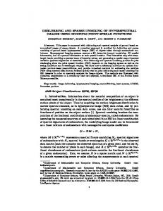
adopted the method called matrix-vector nonnegative tensor factorization for blind unmixing of hyperspectral imagery. Fan et al. [31] proposed a method of hyperspectral image restoration using low-rank tensor recovery. However, it is often the fact that the size of endmember dictionary is much small than the spectral library. In other words, the endmember dictionary is determined by VCA algorithm instead of using spectral library. Recently, to avoid identifying the endmembers in the original hyperspectral data, some researchers use the spectral library as the endmembers and utilize some models based on LRR to estimate the abundance at the same time [32,33]. However, the high mutual coherence of the library signatures makes this model perform badly. It does not distinguish well between the true endmembers and the others. To mitigate the drawback, in this paper, we propose a new hyperspectral unmixing method based on LRR model with dictionary pruning strategy. In addition, most of the traditional models which are based on LRR only take spectral information of hyperspectral data into consideration. The hyperspectral image has special characteristics of space and the information of the space is very important for hyperspectral unmixing. The use of spatial information is concerned with the relationship between each pixel and its neighbours, considering the spatial consistency of the image. Although using spectral information unmixing technology can already obtain very good unmixing results, more previous algorithms using spatial information, such as pre-treatment [34] or unmixing algorithms [35,36], all show the positive impact on the improvement of the unmixing accuracy. To mitigate the drawback, a method which not only considers the global correlation of the data via LRR with space consistency constraint, but also avoids the accurate estimation of the endmembers by pruning the spectral library is proposed in this paper. The proposed algorithm can be described as an iterative process. First, we use the model of the LRR with the space consistency constraint to estimate the abundance while the whole spectral library acting as the endmembers dictionary. Because the number of the real endmembers is much smaller than the whole spectral library, there exists several endmembers whose abundance values are very low. Secondly, we prune the spectral library based on the abundance matrix obtained in the previous step. The pruning strategy follows such an assumption that if the abundance map of one material does not contain any large values, it is not a real endmember and will be removed from the spectral library. After this step, we can get a pruned spectral library which is a subset of the original one. Then, the pruned spectral library is the new endmembers dictionary and the same process in the first step is performed again, and so on. When meeting the stop conditions, the algorithm terminates. Based on the dictionary pruning strategy, the proposed algorithm can use the spectral library as endmembers and avoid extracting them from the hyperspectral image, compared with the algorithm in [36]. In addition, the algorithm can also better capture the spatial structure of data than the sparsity-based unmixing algorithms. The whole process of this method is summarized in Figure 1. The main contributions of our method can be summarized as following. (1) The important characteristic of HSI, space consistency, is integrated in the low-rank representation model for hyperspectral unmixing, which will make the abundance estimation more accurate. (2) A strategy of spectral library pruning is designed by using the coefficients of the low-rank representation, which not only make the result more stable, but also avoids the extraction of endmembers. In addition, we will demonstrate the two advantages in the experiments. The remainder of this paper is organized as follows. In Section 2, we review LMM and introduce the approach. Section 3 describes the proposed methodology. Section 4 analyses the performance of the proposed approach with simulated data and real hyperspectral data. Conclusions are drawn in Section 5.

Remote Sens. 2018, 10, 339 Remote Sens. 2018, 10, x FOR PEER REVIEW

4 of 21 4 of 21

Figure Figure 1. 1. The Theflow flow chart chart of of the the proposed proposed method. method.

2. 2. Related Related Work Work 2.1. 2.1. Linear Linear Spectral Spectral Unmixing Unmixing The The widely widely used used LMM LMM assumes assumes that that the the spectral spectral response response of of aa pixel pixel is is aa linear linear combination combination of of all all the the pure pure spectral spectral signatures signatures (endmembers) (endmembers) present present in in the the pixel. pixel. In In this this case, case, the the model model can can be be described described as: as: m

y=

y=

Ax + n, ∑ ai xxi ++ nn == Ax +n, m

 i =1 a

i

i

(1) (1)

i =1

where y is an L × 1 column vector (the mixed pixel), L is the number of bands, A is an L × m where is an L × 1mcolumn vector (the mixed pixel), L isxthe of bands, A is an the L × fractional m matrix matrixycontaining spectral signatures (endmembers), is anumber m × 1 vector containing containing signaturesand (endmembers), x is adenoting m × 1 vector containing fractional abundancesmofspectral the endmembers, n is an L × 1 vector the noise and modelthe error. abundances of the endmembers, and n is an L × 1 vector denoting the noise and model error. Considering the ground truth, there are two constraints imposed on the LMM: the abundance Considering the ground truth, are two constraints imposed on the LMM: the abundance non-negativity constraint (ANC) andthere the abundance sum-to-one constraint (ASC), respectively: non-negativity constraint (ANC) and the abundance sum-to-one constraint (ASC), respectively: ANC : xi ≥ 0 (i = 1, 2, . . . , m), (2) ANC : x i ≥ 0 (i =1, 2,..., m) , (2) m

ASC :

∑ mxi = 1



(3)

ASC : xi = 1 (3) Let Y ∈ R L× N be the observed image and N isi = 1the total number of mixed pixels in the image. N L× N Let XLet ∈ RYm× the matrix. Equation (1) can be rewritten as:pixels in the image. beabundances the observed imageThen, and N is the total number of mixed ∈ Rbe i =1

Let X ∈ R m× N be the abundances matrix. Then, Equation (1) can be rewritten as:

Remote Sens. 2018, 10, 339

5 of 21

Y = AX + E

(4)

where E ∈ R L× N denoting the noise and model error. In this paper, we will focus on the LMM, due to its computational tractability and flexibility in different applications. 2.2. Abundance Estimation via LRR Abundance estimation via LRR is based on the following theorem [37]. Theorem 1. Assume matrices Y ∈ R L× N , A ∈ R L×m , and X ∈ Rm× N satisfy Y = AX. If rank(Y) = k ≤ min(m,N) and rank(A) = m, then we have: rank(X) = rank(Y) = k

(5)

In [38], the dictionary A is extracted from the hyperspectral image itself. Matrix A usually satisfies the full column rank property as the spectra of the extracted pure endmembers are distinct from each other and the number of bands L is much larger than the number of endmembers m. Normally, the columns of Y are highly correlated and it means that the matrix Y is a low-rank matrix. Thus, we can infer that the corresponding representation matrix X is also low rank. To use this property, researchers employ the LRR model [39,40] to spectral unmixing problem. Starting with the simple LMM, this method can be described as the following optimization problem: X∗ = argminrank(X) , s.t. Y − AX = 0, X ≥ 0, 1T X = 1T

(6)

where Y ∈ R L× N is the observed data matrix, A ∈ R L×m is the endmembers matrix and X ∈ Rm× N is the fractional abundances matrix. X* is the lowest rank solution and the terms X ≥ 0, 1T X = 1T represent the ANC and ASC constraints. Because the rank of the matrix has a discrete type, Equation (6) is not easy to solve. Thus, we can use the nuclear norm of the matrix to replace the rank of the matrix as follows: min X,E

kXk∗ + λkEk2,1

s.t. Y = AX + E, X ≥ 0, 1T X = 1T

,

(7)

where X ∈ Rm× N is the lowest rank representation of the observed signal Y ∈ R L× N , A ∈ R L×m is a linear data space of the dictionary, E ∈ R L× N is the matrix of noise error, the parameter λ is coordination value, k · k∗ is the nuclear norm and k · k2,1 represents the mixed l2,1 norm of the matrix. N is the number of signals, L is the signal dimension, m is the number of dictionary atoms. 2.3. Low-Rank Representation of Coefficient Constraints Low-rank representation is a compressed sensing technology that can effectively restore the original real data, even if the data exist in several sub-spaces. Low-rank representation not only can make full use of the global structure information of the data, but is also robust to noise which has received wide attention since it was put forward. Low-rank representation seeks the lowest rank representation of the observed signal in relative to a suitable dictionary. The basic LRR model with noise is shown in Equation (7). Under normal circumstances, when the dictionary is certain, the similar observation signal has a similar low-rank coefficient. Then, using this property, the regular term is added to the objective function of the basic LRR model. It restricts that similar observation signals have a similar low-rank coefficient. Then, Equation (7) can be modified as follows:

Remote Sens. 2018, 10, x FOR PEER REVIEW

6 of 21

Remote Sens. 2018, 10, 339

6 of 21

m in X,E

X

∗

+λ E

2 ,1

+ β X (I − B )

s.t. Aλ Xk+ min kY Xk=∗ + EkE2,1 +

where I ∈ R

n× n

βkX(I − B)k2F

2 F

(8)

,

X,E , (8) s.t. Y = AX + E is the unit matrix, and ⋅ F is the Frobenius norm of the matrix. The size of matrix B

yi , thenThe is n × In ∈ , and beunit calculated thek method that, if y j isnorm similar to matrix. the size matrix B equals where Rn×itn can is the matrix,by and · k F is the Frobenius of the of matrix B is n × n, and it can be calculated by the method that, if y is similar to y , then the matrix B equals to j i to ωij , or equals to zero, where the ωij is the similarity of the observation vector y i and y j , ωij , or equals to zero, where the ωij is the similarity of the observation vector yi and y j , according to according to the different situations having different construction methods, generally in the range the different situations having different construction methods, generally in the range between 0 and 1, between 0 and 1, more commonly using a heat kernel function and Gauss kernel function. more commonly using a heat kernel function and Gauss kernel function. The regular term added in Equation (8) is to make the similar observation vectors have similar The regular term added in Equation (8) is to make the similar observation vectors have similar LRR coefficients, and the coordination parameter β controls the proportion of the regularization in LRR coefficients, and the coordination parameter β controls the proportion of the regularization in the the whole optimization objective function. The optimization problem of the formula can not only whole optimization objective function. The optimization problem of the formula can not only make make full use of the high correlation among the different bands of the observed data, but also protect full use of the high correlation among the different bands of the observed data, but also protect the the spatial local structure of the data. spatial local structure of the data. 3. Unmixing Unmixing via via LRR LRR Based Based on on Space Space Consistency Consistency Constraint Constraint with with Spectral Spectral Library Library Pruning Pruning 3. 3.1. Space Space Consistency Consistency Constraint Constraint 3.1. In the the previous previous section, section, we we introduce introduce the the method method of of applying applying LRR LRR technique technique to to the the unmixing unmixing In problem, where the VCA is used to extract the endmember dictionary A from the hyperspectral problem, where the VCA is used to extract the endmember dictionary A from the hyperspectral image imageQu itself. Qu et al. [38] proposed this concept, and used solve the problem of unmixing itself. et al. [38] proposed this concept, and used the LRRthe to LRR solvetothe problem of unmixing for the for the first time. In addition, they put forward an improved bilinear model, which applied the LRR first time. In addition, they put forward an improved bilinear model, which applied the LRR to obtain to obtain result of unmixing. the result the of unmixing. In this paper, we propose propose an an algorithm algorithm based based on on LRR LRR with with spatial spatial consistency consistency constraint constraint for for In this paper, we abundance estimation. This algorithm not only makes use of the spectral information of the data, but abundance estimation. This algorithm not only makes use of the spectral information of the data, but also considers considers the the spatial spatial information information of of the the data, data, that that is, is, the the relationship relationship between between the the pixel pixel and and its its also neighbours. It shows the core idea of the algorithm, that is, how we use spatial information in the neighbours. It shows the core idea of the algorithm, that is, how we use spatial information in the process of of unmixing unmixingin inFigure Figure2.2. process

Figure 2. 2. The The schematic schematic for for space space consistency consistency of of hyperspectral hyperspectral image. image. Figure

As can canbebeseen seenfrom from Figure if current the current theobservation i-th observation signal, is, yi , As Figure 2, if2,the pixelpixel is theisi-th signal, that is, ythat i , selecting its n neighbourhoods as its nearest = 3). Typically, current pixel is similar to its spatial selecting its n neighbourhoods as neighbour its nearest (n neighbour (n = 3).the Typically, the current pixel is similar neighbour, but this requires prerequisite, is, the uniform If the current at the to its spatial neighbour, but athis requires athat prerequisite, that is,region. the uniform region. pixel If theiscurrent border, theborder, pixels inthen the red of Figure may belong to two2ormay more substances. pixel isthen at the the box pixels in the 2red box of Figure belong to twoTherefore, or more in addition to the spatial the prior neighbour information, we also to measure substances. Therefore, in neighbour addition toas the spatial as the priorneed information, we the alsodistance need to between the current pixel and its nearest neighbour to distinguish the pixels which are adjacent each measure the distance between the current pixel and its nearest neighbour to distinguish thetopixels other to different kinds.but As belong shown in 2, the 3 ×As 3 neighbourhood of 2, thethe current whichbut arebelong adjacent to each other to Figure different kinds. shown in Figure 3× 3 pixel has a total of pixels, the pixel ihas is at the boundary, and thei is j-th, k-thboundary, and m-th endmembers neighbourhood of8the current a total of 8 pixels, theonly pixel at the and only the are same the pixel i. At this is needed judge bythis the point, distance measure j-th,the k-th andkind m-thofendmembers are thepoint, sameitkind of theto pixel i. At it is neededtotoavoid judgethe by condition that the boundary is misidentified as the homogeneous region. The detail of measurement

Remote Sens. 2018, 10, 339

7 of 21

process is: first, calculate the Euclidean distance between the current pixel and its nearest neighbour, and then, select the nearest p pixels as the real neighbour of the current pixel. In summary, the so-called spatial consistency constraint reflects the following facts: (1) (2) (3)

The pixels of the near neighbourhood in the image have similar endmembers and their corresponding abundance. The pixels of the near spectral distance have similar endmembers and their corresponding abundance. At the same time, combined with the above two points, selecting p pixels with the nearest distance to the current pixels in the n neighbourhood as its real neighbourhood, constrain its abundances to be similar.

The above thoughts are shown to be of great advantage through experiments. If we only consider the first point, we cannot avoid the boundary problem which will cause the error increase. Because of the presence of noise and the interference of the atmosphere, even though the spectral information of the pixels is very similar, but they are also likely to belong to the different materials. Thus, it is not appropriate to only consider the second point. The combination of the first point and the second point at the same time is the key for the algorithm to improve the accuracy of unmixing. Then, we propose an optimization model based on the LRR with the spatial consistency constraint for the estimation of the abundance as follows: min kXk∗ + λkEk2,1 + βkX( pI − B)k2F X,E

s.t. Y = AX + E, X ≥ 0, 1T X = 1T

,

(9)

where Y ∈ R L× N is the hyperspectral data, X ∈ R L×m is the abundance matrix, E ∈ R L× N is the noise matrix, and ∈ R N × N is the unit matrix. The λ and β are coordinate parameters, m is the number of the endmember and p refers to the p pixels of the nearest distance to the current pixel in n × n neighbourhood of the current pixel as its real neighbour. The size of matrix B is n × n, and it can be calculated by the method that if y j is similar to yi , then the matrix B equals to ωij , or equals to zero, where ωij is the similarity of the observation vector yi and y j . We set ωij to be 1. The optimization problem shown in Equation (9) can be solved by the method of Augmented Lagrange Multiplier (ALM) [41]. The ANC is added in each step of the iterative process, while the ASC is embodied in the normalization process of the last step of the iteration. Because the ANC has obvious physical meaning, that is, the value of abundance cannot be negative, so the general situation is to add it. The ASC need to choose to add or not based on the actual situation. The whole solving process of the optimization problem is as follows. Firstly, we remove the ANC and the ASC of Equation (9), and translate it into the following equivalent problem: min

kJk∗ + λkEk2,1 + βkLHk2F

st.

Y = AX + E, J = X H = pI − B, L = X

Z,E,J

(10)

Then, Equation (10) can be converted to the ALM problem as follows: min

X,E,J,L,Y1 ,Y2

kJk∗ + λkEk2,1 + βkLHk2F + tr [Y1T (Y − AX − E)] + tr [Y2T (X − J)] + tr [Y3T (X − L)]+ , µ 2 2 2 2 (kY − AX − Ek F + kX − Jk F + kX − Lk F )

(11)

where Y1 , Y2 and Y3 are the Lagrangian multipliers, and µ is the penalty parameter. For efficiency, we choose the inexact ALM, which we outline in Algorithm 1.

Remote Sens. 2018, 10, 339

8 of 21

Algorithm 1: Solve the SCC-LRR problem by ALM Input: library A, data matrix Y, near neighbourhood consistency constraint matrix H, and regularization parameter λ, β. Initialize: X = J = L = 0, E = 0, Y1 = 0, Y2 = 0, Y3 = 0, µ = 10–6, maxu = 1010, ρ = 1.1, ε = 10–8. while not converged do 1: Fix the others and update J by J = argmin µ1 kJk∗ + 12 kJ − (X + Y2 /µ)k2F , J = max(J, 0). −1

2: Fix the others and update X by X = (2I + At A) (At Y − At E + J + L + (At Y1 − Y2 − Y3 )/µ). 3: Fix the others and update E by E = argmin λµ kEk2,1 + 21 kE − (Y − AX + Y1 /µ)k2F . −1

4: Fix the others and update L by L = (µX + Y3 )(2βHHT + µI) . 5: Update the multipliers Y1 = Y1 + µ(Y − AX − E)Y2 = Y2 + µ(X − J)Y3 = Y3 + µ(X − L). 6: Update the parameter µ by µ = min(ρµ, maxµ ). 7: check the convergence condition kY − AX − Ek∞ < ε &kX − Jk∞ < ε &kX − Lk∞ < ε. end Output: representation coefficient X.

3.2. Spectral Library Pruning After solving optimization (Equation (9)), we can obtain the fractional abundances matrix X corresponding to the spectral library A. Compared with the size of the spectral library, the number of endmembers in a given scene is usually much smaller. Thus, sparsity exists among the lines of the obtained abundances matrix X and each line of X denotes the abundance map corresponds to one endmember. To utilize the sparsity, we propose a dictionary pruning strategy to prune the abundances matrix X and its corresponding spectral signatures in A. This strategy can be described as two steps: (1) (2)

Compute the number of the pixels whose abundance value corresponding to one endmember is smaller than a preset threshold denoted by ε. If the number is equal to the total number of pixels in the scene, we will get rid of the spectral signature from the endmember matrix.

It means that if one endmember is rarely distributed over the scene, it is not a real endmember. In general, if one spectral signature is a real endmember, its abundance values corresponding to some areas will be high in some areas in the scene. That is our motivation of using the strategy to prune the spectral library A. In the experiments on simulated data, we set ε to be 0.02 and then if one endmember is distributed under 2% over the scene, it will be removed from the library. The value of ε should be set to a small value to avoid removing the true endmembers from the library. Thus, we set ε to 0.01 in the experiments of real data because real data are more complex than simulated data. In each iteration, the size of spectral library will decrease and the abundances of the retained endmembers will increase. Thus, in each iteration, the value of ε will be updated by ε × iterations. Then, we can get a pruned spectral library A as the endmember matrix in which the number of spectral signatures is smaller than the original one. By using this pruned spectral library A, we solve the optimization (Equation (9)) again and obtain a new fractional abundances matrix Y corresponding to the pruned spectral library A. According to the dictionary pruning strategy, we can prune the spectral library A repeatedly until the number of spectral signatures retained meets the stopping condition. A threshold denoted by T acting as the stop condition is defined to control this iterative process. The stop condition can be described like that when the difference between the number of spectral signatures retained and the estimated number of endmembers in a scene is less than T, the algorithm stops. Thus, a higher value of T means that it retains more endmembers from the spectral library. In this paper, we use the hyperspectral subspace identification by minimum error (HySime) algorithm [42] to estimate the number of endmembers. In the experiments with simulated data, the range of values for T is 1 to 10 and in the experiments with real data, we set T to be 25. We retain more endmembers for real data because they are more complex than simulated data. When the situation is complex (e.g., low

Remote Sens. 2018, 10, 339

9 of 21

SNR, big endmember number or a very large library), we set ε to be a small value and T be a large value to avoid removing the true endmembers from the library. After several iterations, we can get a good result of the optimization problem. The whole process of this method has been summarized in Figure 1. 4. Experiments with Simulated Data and Real Data To validate the two main advantages of our method, the space consistency and the strategy of spectral pruning, we first compare the method of LRR with our proposed method to validate the effectiveness of the space consistency constraint for abundance estimation, and we also show the spectral library pruned by our method to demonstrate the effectiveness of the spectral library pruning strategy. In Section 4.1, we use three simulated datasets to analyse the performance of the proposed approach. Firstly, we introduce the three datasets, and then we analysis the performances of them separately including the parameter settings, error analysis, etc. In Section 4.2, we use the real dataset and analyse its performance with other traditional methods. Finally, we analyse the parameters of the experiments in Section 4.3. The results of the experiments show the good performance of the proposed method. 4.1. Simulated Datasets The spectral library we used in our simulated image experiments is generated from a random selection of 240 materials from the USGS library, denoted splib061 and released in September 2007. It comprises spectral signatures with reflectance values given in 224 spectral bands and distributed uniformly in the interval 0.4–2.5 µm. Our library, denoted by A1, is used to generate three different simulated hyperspectral data cubes. (1)

(2)

(3)

Simulated Data Cube 1 (DC1): This simulated data cube is generated following the methodology of [26], using five randomly selected spectral signatures from A1. DC1 has 75 × 75 pixels and each simulated pixel was generated using a LMM, with the five endmembers and imposing the ASC in it. In the resulting simulated image, shown in Figure 3a, there are pure regions as well as mixed regions constructed using mixtures ranging between two and five endmembers, distributed spatially in the form of distinct square regions. Figure 3b–f, respectively, shows the true fractional abundances for each of the five endmembers. The background pixels are made up of mixtures of the same five endmembers, but their respective fractional abundances values were randomly fixed as 0.1149, 0.0741, 0.2003, 0.2055 and 0.4051, respectively. The obtained data cube was then contaminated with white noise, having different levels of the signal-to-noise ratio (SNR): 20, 30 and 40 dB. Simulated Data Cube 2 (DC2): Using the library A1, we generated a data cube of 48 × 48 pixels and it contains six endmembers. The endmembers were randomly selected from library A1. In each simulated pixel, the fractional abundances of the endmembers follow a Dirichlet distribution [14]. As DC1, the scene was again contaminated with white noise using the same SNR value adopted for DC1. Simulated Data Cube 3 (DC3): Using the library A1, we generate various data cubes of 75 × 75 pixels, each containing five endmembers. The simulated method is similar to the first simulated data. There are pure regions as well as mixed regions constructed using mixtures ranging between two and five endmembers, distributed spatially in the form of distinct square regions. The background pixels are made up of mixtures of the same five endmembers, but their respective fractional abundances values were randomly fixed as 0.1149, 0.0741, 0.2003, 0.2055 and 0.4051, respectively. The obtained data cube was then contaminated with white noise

pixels, each containing five endmembers. The simulated method is similar to the first simulated data. There are pure regions as well as mixed regions constructed using mixtures ranging between two and five endmembers, distributed spatially in the form of distinct square regions. The background pixels are made up of mixtures of the same five endmembers, but their respective fractional abundances values were randomly fixed as 0.1149, 0.0741, 0.2003, 0.2055 Remote Sens. 2018, 10, 339 10 of 21 and 0.4051, respectively. The obtained data cube was then contaminated with white noise

Figure fractional abundances of endmembers in the in simulated data cube 1 (DC1): simulated Figure3.3.True True fractional abundances of endmembers the simulated data cube (a) 1 (DC1): (a) image; (b) the true abundance of endmember 1; (c) the true abundance of endmember 2; (d) the true simulated image; (b) the true abundance of endmember 1; (c) the true abundance of endmember 2; abundance endmember (e) the true3;abundance of abundance endmemberof4;endmember and (f) the true abundance of (d) the trueofabundance of 3; endmember (e) the true 4; and (f) the true endmember 5. endmember 5. abundance of

In In this this work, work, the the proposed proposed algorithm algorithm is is tested tested on on three three groups groups of of simulated simulated datasets datasets and and aa real real hyperspectral hyperspectral image. image. To verify verify the the superiority superiority of of the the proposed proposed algorithm, algorithm, the the performance performance of of itit is is compared compared with with both both the the traditional traditional unmixing unmixing algorithms algorithms (nonnegative (nonnegative constrained constrained least least squares squares (NCLS), squares (FCLS)) [11][11] andand the the sparse unmixing algorithms (SUnSAL [17], (NCLS),full fullconstrained constrainedleast least squares (FCLS)) sparse unmixing algorithms (SUnSAL SUnSAL-TV [23] and CLSUnSAL [26]). The parameter threshold ε plays an important role in [17], SUnSAL-TV [23] and CLSUnSAL [26]). The parameter threshold ε plays an important rolethe in proposed algorithm and and we set to it 0.02 in our image experiments. the proposed algorithm weitset to 0.02 in simulated our simulated image experiments. The The quality quality metric metric adopted adopted in in our our experiments experiments to to assess assess the the unmixing unmixing results results is is the the signal signal to to reconstruction reconstructionerror error(SRE) (SRE)[17], [17],which whichcan canbe bedefined definedas asfollows: follows: 2

E[ x 2 ]2 ] 2 ) log10( ( E[kxk = 10 ), SRESRE = 10 log 2 10 E[ x − x ˆ E[kx − xˆ2k]22 ],

(12) (12)

where fractionalabundance abundancevector vectorand and xˆ isisthe where X X is the true fractional theestimated estimatedfractional fractional abundance abundance vector. EE(·) Thehigher higherthe theSRE SREis,is,the thebetter betterthe the quality unmixing is. it Ascan it standsfor for mean mean value. The quality of of thethe unmixing is. As (⋅) stands can give more information regarding the power of the signal in relation with the power of the error, give more information regarding the power of the signal in relation with the power of the error, we we measure instead of the classical mean squared error (RMSE) compute useuse thisthis measure instead of the classical rootroot mean squared error (RMSE) [34].[34]. WeWe alsoalso compute the the abundance angle distance (AAD) as another performance discriminator adopted this paper. abundance angle distance (AAD) as another performance discriminator adopted in thisinpaper. AAD AAD can express as follows: can express as follows: ! xit · xˆ it 1 m −1 AAD = ∑ cos , m i =1 kxi k · kxˆ i k

(13)

where Xi is the true fractional abundance vector of the i-th endmember and xˆ i is the estimated fractional abundance vector of the i-th endmember. m stands for the number of the endmembers. Figure 4 shows the abundance maps obtained by different unmixing methods for endmember #5 in DC1. Throughout the estimated abundance results, the abundance maps obtained by NCLS and SUnSAL are full of noise points and it is hard to make out the endmember signature from the mixed

m

i =1

 x i ⋅ xˆ i  ,

where Xi is the true fractional abundance vector of the i-th endmember and

xˆ i

is the estimated

fractional abundance vector of the i-th endmember. m stands for the number of the endmembers. 4 shows RemoteFigure Sens. 2018, 10, 339 the abundance maps obtained by different unmixing methods for endmember 11 of 21 #5 in DC1. Throughout the estimated abundance results, the abundance maps obtained by NCLS and SUnSAL are full of noise points and it is hard to make out the endmember signature from the spectral. The reason this is A1library is generated a random of mixed spectral. The for reason forthat thistheisspectral that thelibrary spectral A1 is from generated fromselection a random 240 materials from the USGS library. The spectral angle distance is quite small, which makes it difficult selection of 240 materials from the USGS library. The spectral angle distance is quite small, which to separate the endmembers noise. Since DC1 has distinct spatial SUnSAL-TV, which makes it difficult to separatefrom the endmembers from noise. Since DC1 information, has distinct spatial information, considers spatial information, achieves a better result than NCLS and SUnSAL. The abundance maps SUnSAL-TV, which considers spatial information, achieves a better result than NCLS and SUnSAL. obtained by SUnSAL-TV have smoother spatial changes in the homogeneous regions, and contain The abundance maps obtained by SUnSAL-TV have smoother spatial changes in the homogeneous fewer noise in points. some cases, the abundance images obtained byimages SUnSAL-TV may regions, andpoints. containHowever, fewer noise However, in some cases, the abundance obtained by exhibit an over-smooth visual effect in some regions. SUnSAL-TV may exhibit an over-smooth visual effect in some regions.

Figure 4. 4. Abundance Abundance maps maps obtained obtained by by different different unmixing unmixing methods methods for for endmember endmember #5 #5 in in DC1 DC1 and, and, Figure from top to bottom, SNR is 20 dB, 30 dB, and 40 dB. from top to bottom, SNR is 20 dB, 30 dB, and 40 dB.

In Table 1, we can also find that LRR model performs about similar to SUnSAL in the unmixing In Table 1, we can also find that LRR model performs about similar to SUnSAL in the unmixing problem. LRR model can capture global structures of the abundance matrix and is also robust to problem. LRR model can capture global structures of the abundance matrix and is also robust to noise. However, due to the large library and its high mutual coherences, LRR does not perform noise. However, due to the large library and its high mutual coherences, LRR does not perform much better than SUnSAL. In addition, the method based on the LRR with the space consistency much better than SUnSAL. In addition, the method based on the LRR with the space consistency constraint (SCC-LRR) also achieves a better result than the other methods besides the proposed constraint (SCC-LRR) also achieves a better result than the other methods besides the proposed method. method. The reason is that there are some homogeneous regions in DC1 and the method of the The reason is that there are some homogeneous regions in DC1 and the method of the SCC-LRR takes SCC-LRR takes the space consistency into consideration. Due to consideration of the space the space consistency into consideration. Due to consideration of the space consistency constraint and consistency constraint and the dictionary pruning strategy, the abundance maps obtained by the the dictionary pruning strategy, the abundance maps obtained by the proposed algorithm are closer to proposed algorithm are closer to the true abundance maps than the ones estimated by SUnSAL-TV. the true abundance maps than the ones estimated by SUnSAL-TV. As shown in Table 1, the accuracy As shown in Table 1, the accuracy of the results is clearly improved when the proposed algorithm is of the results is clearly improved when the proposed algorithm is used. Therefore, the proposed used. Therefore, the proposed algorithm significantly outperforms the other methods. algorithm significantly outperforms the other methods. According to the comparative analysis of the experiment, the selections of n = 3 and p = 3 are more According to the comparative analysis of the experiment, the selections of n = 3 and p = 3 are appropriate. When n = 5, the experiment shows that the effect is not improved and there are more more appropriate. When n = 5, the experiment shows that the effect is not improved and there are calculations. In addition, it will lead to the advantage of space consistency not not being easily more calculations. In addition, it will lead to the advantage of space consistency not not being easily reflected when the value of p is too small. On the contrary, if the value of p is too large, it will cause a greater error. In addition, the optimal setting and running times are shown in Table 2. To validate the proposed algorithm extensively, we use DC2 to demonstrate the effectiveness. Figure 5 shows the ground-truth and the estimated abundances obtained by different unmixing methods in the A1 library. The datasets contain six true endmembers and the positions of the true endmembers in the original library are 5, 6, 26, 34, 67 and 177, as shown in Figure 5a. In Figure 5,

Remote Sens. 2018, 10, 339

12 of 21

it can be seen graphically that the lines (denoting the abundance of a certain endmember in all pixels of the image) estimated by CLSUnSAL are more sparse than the ones estimated by SUnSAL. After applying SUnSAL, as shown in Figure 5b, there are many low abundance values estimated for endmembers which are not actually present in the image. Due to the high mutual coherence of the library signatures, SUnSAL does not perform well. Unlike SUnSAL, which employs pixelwise independent regression, CLSUnSAL enforces joint sparsity among all the pixels. Thus, it improves significantly the accuracy of the unmixing solutions over those provided by SUnSAL. Although the abundances obtain by CLSUnSAL are similar to those in the ground-truth, there are also several lines that are not true abundances in Figure 5c. Figure 5d shows the estimated abundances obtained by the proposed algorithm. After applying this method, the remained subset of the spectral library contains six endmembers. However, almost every line of the image is much brighter than the one in the true abundance map. This is because that the image in DC2 contains very few homogeneous regions, which leads to the failure of spatial consistency constraints. However, it improves the accuracy in the whole, which is shown in Table 3. Table 1. SRE (dB) and AAD values achieved after applying different unmixing methods to Simulated DATA 1. Methods

DC1

SNR = 20 dB

SNR = 30 dB

SNR = 40 dB

NCLS

SRE AAD

1.2648 0.8512

2.5000 0.5657

7.5332 0.2211

SUnSAL

SRE AAD

1.5753 0.8276

3.2432 0.6414

8.2820 0.1853

SUnSAL-TV

SRE AAD

5.5956 0.4530

15.0211 0.0486

23.6639 0.0206

LRR

SRE AAD

1.6232 0.4777

3.5426 0.2779

6.7140 0.1401

SCC-LRR

SRE AAD

2.8598 0.1838

5.1026 0.0753

4.8676 0.1823

SLP-SCC-LRR

SRE AAD

21.8418 0.0318

32.7520 0.0221

44.5256 0.0074

Table 2. The optimal parameters settings and running times(s) with the Simulated DATA 1. Methods

DC1

SNR = 20 dB

SNR = 30 dB

SNR = 40 dB

NCLS

Times

41.8314

28.7967

23.2396

SUnSAL

Parameters Times

λ = 8 × 10−2 21.2719

λ = 8 × 10−2 22.4660

λ = 1 × 10−2 24.2318

Times

λ = 5 × 10−2 λTV = 5 × 10−2 523.0716

λ = 5 × 10−3 λTV = 1 × 10−2 527.0992

λ = 3 × 10−3 λTV = 5 × 10−3 611.4388

Parameters Times

λ = 0.5 861.1286

λ=4 936.9994

λ = 70 784.9693

λ=6 β = 100 232.0626

λ =15 β = 110 246.2892

λ=6 β = 100 264.2972

λ=6 β = 100 T=3 400.3627

λ = 15 β = 110 T=2 374.6602

λ=6 β = 100 T=1 412.6240

SUnSAL-TV

LRR

SCC-LRR

Parameters

Parameters Times

SLP-SCC-LRR

Parameters Times

Remote Sens. 2018, 10, 339 Remote Sens. 2018, 10, x FOR PEER REVIEW

13 of 21 13 of 21

Figure 5. Ground-truth and estimated abundances obtained by different unmixing methods in the Figure 5. Ground-truth and estimated abundances obtained by different unmixing methods in the scene DC2, with SNR = 40 dB: (a) ground-truth abundance; (b) estimated abundances obtained by scene DC2, with SNR = 40 dB: (a) ground-truth abundance; (b) estimated abundances obtained by SUnSAL; (c) estimated abundances obtained by CLSUnSAL; and (d) estimated abundances obtained SUnSAL; (c) estimated abundances obtained by CLSUnSAL; and (d) estimated abundances obtained by by SLP-SCC-LRR. SLP-SCC-LRR. Table 3. SRE (dB) and AAD values achieved after applying different unmixing methods to Table 3. SRE (dB) and AAD values achieved after applying different unmixing methods to Simulated Simulated DATA 2. DATA 2. Methods (DC2) Methods (DC2) SUnSAL CLSUnSAL SUnSAL LRR CLSUnSAL SCC-LRR LRR SMP + SUnSAL SCC-LRR SMP + CLSUnSAL SMP + SUnSAL + LRR SMPSMP + CLSUnSAL SMP + SCC-LRR SMP + LRR RSFoBa + SUnSAL SMP + SCC-LRR RSFoBa + CLSUnSAL RSFoBa + SUnSAL RSFoBa + LRR RSFoBa + CLSUnSAL RSFoBa + SCC-LRR RSFoBa + LRR SLP ++SUnSAL RSFoBa SCC-LRR SLP + CLSUnSAL SLP + SUnSAL SLP +SLP-LRR CLSUnSAL SLP-SCC-LRR SLP-LRR SLP-SCC-LRR

SNR = 20 dB SNR = 20 dBAAD SRE 1.7227 0.9619 SRE AAD 2.1666 0.7251 1.7227 0.9619 1.7299 0.5822 2.1666 0.7251 0.4881 0.6004 1.7299 0.5822 2.1126 0.8923 0.6004 0.4881 2.9256 0.8083 2.1126 0.8923 1.8926 0.5424 2.9256 0.8083 0.4881 0.6582 1.8926 0.5424 2.3032 0.8520 0.6582 0.4881 2.8469 0.6162 2.3032 0.8520 0.4672 2.5989 2.8469 0.6162 0.7044 0.4881 2.5989 0.4672 4.9159 0.5632 0.7044 0.4881 0.3010 3.6273 4.9159 0.5632 5.3920 0.3386 3.6273 0.3010 4.4974 0.4054 5.3920 0.3386 4.4974 0.4054

SNR = 30 dB SNR dB SRE = 30 AAD 3.1024 0.7060 SRE AAD 4.0155 0.4013 3.1024 0.7060 3.0060 0.3143 4.0155 0.4013 0.2931 1.3476 3.0060 0.3143 3.4765 0.6654 1.3476 0.2931 4.3575 0.2092 3.4765 0.6654 3.0206 0.3123 4.3575 0.2092 1.4118 0.2931 3.0206 0.3123 5.4326 0.4982 1.4118 0.2931 9.6058 0.1628 5.4326 0.4982 5.4969 0.3503 9.6058 0.1628 1.6437 0.2931 5.4969 0.3503 18.9343 0.2931 0.1100 1.6437 19.0567 0.1090 18.9343 0.1100 0.1090 19.0560 0.1090 19.0567 19.0002 0.1097 19.0560 0.1090 19.0002 0.1097

SNR = 40 dB SNR = 40 dB SRE AAD 6.0602 0.3963 SRE AAD 9.4707 0.0958 6.0602 0.3963 4.0263 0.1781 9.4707 0.0958 1.7065 0.2102 4.0263 0.1781 6.9170 0.3579 1.7065 0.2102 7.6023 0.2367 6.9170 0.3579 0.1866 4.7494 7.6023 0.2367 1.7759 0.2102 4.7494 0.1866 11.5092 0.2134 1.7759 0.2102 20.3783 0.0521 11.5092 0.2134 9.8677 20.3783 0.1443 0.0521 1.9177 0.2102 9.8677 0.1443 0.0363 28.5571 1.9177 0.2102 28.4343 28.5571 0.0367 0.0363 28.5731 28.4343 0.0363 0.0367 28.4715 28.5731 0.0366 0.0363 28.4715 0.0366

Using DC2, we also demonstrate the effectiveness of the space consistency and the dictionary pruning method separately. In Table the 3, we can find that, usingconsistency the whole and library A1 as the Using DC2, we also demonstrate effectiveness of theifspace the dictionary endmembers matrix, CLSUnSAL can obtain the highest SRE (dB) values. This is because CLSUnSAL pruning method separately. In Table 3, we can find that, if using the whole library A1 as the constrains the pixels to share the same set of endmembers. AAD is defined as the angle between estimated abundances and the true abundances. The AAD values achieved by LRR are lower than

Remote Sens. 2018, 10, 339

14 of 21

endmembers matrix, CLSUnSAL can obtain the highest SRE (dB) values. This is because CLSUnSAL constrains the pixels to share the same set of endmembers. AAD is defined as the angle between estimated abundances and the true abundances. The AAD values achieved by LRR are lower than those of the other methods when the observed data have a lower SNR. This is because LRR can capture the global structures of the abundance matrix. Some other methods exploit pruning methods in unmixing with given spectral library. Zortea and Plaza [34] use the array processing methodologies to prune the spectral library effectively while the greedy algorithms proposed in [43,44] can also be taken as dictionary pruning methods to boost sparse unmixing algorithms. Thus, we compare the results obtained by our proposed dictionary pruning method to those obtained with subspace matching pursuit (SMP) algorithm [43] and regularized simultaneous forward-backward greedy algorithm (RSFoBa) [44]. The numbers of potential endmembers retained from the original library by the SMP method are 148 (SNR = 20 dB), 167 (SNR = 30 dB) and 162 (SNR = 40 dB), respectively. The numbers of endmembers retained by the RSFoBa method are 100 (SNR = 20 dB), 64 (SNR = 30 dB) and 42 (SNR = 40 dB), respectively. In Table 3, we can conclude that both SMP and RSFoBa can improve the unmixing algorithm performance compared with those algorithms using the original large spectral library for unmixing. Since the size of sub-library obtained by the RSFoBa is smaller than that by SMP and both the sub-libraries contain true endmembers, RSFoBa makes the unmixing algorithms more accurate than SMP, as shown in Table 3. In our proposed algorithm, threshold T acting as the stop condition controls the size of retained subset of the spectral library. We set it to be 1 to 10 in the experiments so that the retained endmembers will not be 10 more than the estimated number of endmembers in a scene. The parameters of the DC2 are shown in Table 4. Especially, when the observed data have high SNR levels, our proposed dictionary pruning method can select the true endmembers accurately from the original large spectral library. Thus, we can also find the potential of our proposed dictionary pruning method can select the true endmembers accurately from the original large spectral library. Besides, we can also find the potential of our proposed dictionary pruning method which can boost the performances of the other unmixing algorithms. Table 4. The optimal parameters settings and running times(s) with the Simulated DATA 2. Methods (DC2)

SNR = 20 dB Parameters

SUnSAL CLSUnSAL LRR SCC-LRR SMP + SUnSAL SMP + CLSUnSAL SMP + LRR SMP + SCC-LRR RSFoBa + SUnSAL RSFoBa + CLSUnSAL RSFoBa + LRR RSFoBa + SCC-LRR SLP + SUnSAL SLP + CLSUnSAL SLP-LRR SLP-SCC-LRR

Times

λ = 0.05 λ = 0.9 λ=2 λ=2 β = 0.01

16.9724 40.8787 206.4049

λ = 0.08 λ=2 λ=2 λ =2 β = 0.01

6.4694 11.8081 64.0299

λ = 0.03 λ = 0.2 λ=2 λ=2 β = 0.01 λ = 0.05 T = 10 λ=2 T = 10 λ=2 T = 10 λ=2 β = 0.01 T = 10

122.5415

114.3858 3.1553 19.9172 54.3540 118.9212 76.3745 25.0145 689.9156 290.9236

SNR = 30 dB Parameters

Times

λ = 0.01 λ = 0.2 λ = 20 λ = 36 β = 0.1

11.6911 41.5278 182.7591

λ = 0.01 λ = 0.2 λ = 10 λ =36 β = 0.1

6.1948 12.5174 73.1744

λ = 4 × 10−3 λ = 0.2 λ = 35 λ = 36 β = 0.1 λ = 6 × 10−3 T=1 λ = 0.1 T=1 λ=8 T=1 λ = 36 β = 0.1 T=1

109.7295

111.7261 1.9873 9.6373 35.4342 118.7259 45.0329 33.0251 471.5313 489.6472

SNR = 40 dB Parameters 10−3

λ=1× λ = 0.05 λ = 50 λ=6 β = 0.01

λ = 9 × 10−4 λ = 8 × 10−3 λ = 80 λ=6 β = 0.01 λ = 6 × 10−4 λ = 0.1 λ = 80 λ=6 β = 0.01 λ = 1 × 10−3 T=1 λ = 0.04 T=1 λ = 80 T=1 λ=6 β = 0.01 T=1

Times 8.7732 41.3956 164.0270 117.2215 4.6662 12.5302 79.6736 123.7080 0.8679 6.0128 21.1428 128.7818 19.0163 23.7061 324.2536 323.6368

Remote Sens. 2018, 10, 339 Remote Sens. 2018, 10, x FOR PEER REVIEW

15 of 21 15 of 21

Then, we the proposed proposedmethod methodon onthe theDC3, DC3, shown Figure Then, wealso alsotest testthe theperformance performance of the asas shown in in Figure 6. 6. Figure 6 shows the simulated datathe and the true fractional abundances forthe each the five Figure 6 shows the simulated data and true fractional abundances for each of fiveof endmembers. endmembers. There are both homogeneous region and heterogeneous region,inasFigure shown6a. in Figure There are both homogeneous region and heterogeneous region, as shown Figure6a. 6b–f Figure the true of the five endmembers. 7a–e shows the shows the6b–f true shows abundance mapsabundance of the five maps endmembers. Figure 7a–e showsFigure the estimated abundance estimated abundance maps obtained by which the proposed method, which contains five endmembers. maps obtained by the proposed method, contains five endmembers. Considering the sparse Considering the sparse consistency constraint, the pixel of the heterogeneous region is not similar to consistency constraint, the pixel of the heterogeneous region is not similar to its neighbour pixels which its neighbour pixels which will makes the effect of the unmixing become worse, as shown in Figure will makes the effect of the unmixing become worse, as shown in Figure 7. On the contrary, in the 7. On the contrary, inthe the effects homogeneous region, thecan effects of the unmixing can7, bethe obtained. In Figure homogeneous region, of the unmixing be obtained. In Figure proposed method 7, the proposed method can obtain better results overall. We also compare the results with the other can obtain better results overall. We also compare the results with the other methods, as shown in methods, as shown in Table 5. In addition, the parameter setting and the time of the iterations are Table 5. In addition, the parameter setting and the time of the iterations are shown in Table 5. In Table 5, shown in Table 5. In Table 5, we can find that our method has better performance than other we can find that our method has better performance than other traditional methods. However, the traditional methods. However, the time of running is higher, which we need to improve in the time of running is higher, which we need to improve in the future. future. Table 5. SRE (dB) and AAD values to Simulated Dataset 3 with the parameter settings and Table 5. SRE (dB) and AAD values to Simulated Dataset 3 with the parameter settings and running running times. times. Methods Methods LRR LRR SUnSAL SUnSAL SUnSAL-TV SUnSAL-TV SCC-LRR SCC-LRR SLP-SCC-LRR SLP-SCC-LRR

DC3 DC3 SRE SRE AAD AAD SRE SRE AAD AAD SRE SRE AAD AAD SRE SRE AAD AAD SRE

SNR SNR = = 40 40 dB dB 0.2997 0.2997 1.1210 1.1210 0.2419 0.2419 1.2584 1.2584 0.0971 0.0971 0.9397 0.9397 0.4061 0.4061 0.8596 0.8596 22.3349

AAD AAD

0.0903 0.0903

SRE

22.3349

Parameters Parameters

Times Times

−1 λλ ==11 ××10 10−1

486.9841 486.9841

−2 λλ ==11 ××10 10−2

11.4843 11.4843

λλ==1 1 −2 λ TV = λTV =55××1010−2 λλ==1010 ββ==5050 λλ == 1 β β= =111 111 TT==11

228.4922 228.4922 232.9945 232.9945 840.1768 840.1768

Figure 6. True fractional abundances of endmembers in the simulated data cube 3 (DC3): (a) Figure 6. True fractional abundances of endmembers in the simulated data cube 3 (DC3): (a) simulated simulated image; (b) the true abundance of endmember 1; (c) the true abundance of endmember 2; image; (b) the true abundance of endmember 1; (c) the true abundance of endmember 2; (d) the true (d) the true abundance of endmember 3; (e) the true abundance of endmember 4; and (f) the true abundance of endmember 3; (e) the true abundance of endmember 4; and (f) the true abundance of abundance of endmember 5. endmember 5.

Remote Sens. 2018, 10, 339 Remote Sens. 2018, 10, x FOR PEER REVIEW

16 of 21 16 of 21

Figure 7. Abundance maps obtained by the proposed unmixing method in DC3 and the SNR is 40 Figure 7. Abundance maps obtained by the proposed unmixing method in DC3 and the SNR is 40 dB: dB: (a) the true abundance of endmember 1; (b) the true abundance of endmember 2; (c) the true (a) the true abundance of endmember 1; (b) the true abundance of endmember 2; (c) the true abundance abundance of endmember 3; (d) the true abundance of endmember 4; and (e) the true abundance of of endmember 3; (d) the true abundance of endmember 4; and (e) the true abundance of endmember 5. endmember 5.

In In summary, summary, from from the the qualitative qualitative and and quantitative quantitative comparison comparison between between the the results results obtained obtained by by these methods, we can conclude that the proposed algorithm offers more promising results than the these methods, we can conclude that the proposed algorithm offers more promising results than the other However, furtherfurther experiments should beshould conducted real hyperspectral other unmixing unmixingmethods. methods. However, experiments be with conducted with real scenes to fully scenes substantiate our findings inour realfindings scene. in real scene. hyperspectral to fully substantiate 4.2. Real Datasets 4.2. Real Datasets The scene used in our real data experiments is the well-known AVIRIS Cuprite Dataset in The scene used in our real data experiments is the well-known AVIRIS Cuprite Dataset in west-central Nevada in 1997. This scene has been widely used to validate the performance of unmixing west-central Nevada in 1997. This scene has been widely used to validate the performance of algorithms. The portion used in experiments corresponds to a 250 × 191-pixel subset of the data. unmixing algorithms. The portion used in experiments corresponds to a 250 × 191-pixel subset of the Due to water absorption and low SNR, the number of spectral bands is reduced from 224 to 188. data. Due to water absorption and low SNR, the number of spectral bands is reduced from 224 to For illustrative purposes, Figure 8 shows a mineral map produced in 1995 by USGS. Although the 188. For illustrative purposes, Figure 8 shows a mineral map produced in 1995 by USGS. Although map is available for hyperspectral data collected in 1995 and the publicly available AVIRIS Cuprite the map is available for hyperspectral data collected in 1995 and the publicly available AVIRIS data were collected in 1997, the USGS map serves as a good indicator for qualitative assessment of the Cuprite data were collected in 1997, the USGS map serves as a good indicator for qualitative fractional abundance maps produced by the different unmixing algorithms. assessment of the fractional abundance maps produced by the different unmixing algorithms. The standard spectral library for these data, denoted by A, is the USGS library containing The standard spectral library for these data, denoted by A, is the USGS library containing 498 498 pure endmember signatures. Before unmixing the real hyperspectral data, essential calibration pure endmember signatures. Before unmixing the real hyperspectral data, essential calibration was was undertaken to mitigate the mismatches between the hyperspectral image and the signatures in the undertaken to mitigate the mismatches between the hyperspectral image and the signatures in the library [17]. library [17]. Figure 9 shows a comparison between the fractional abundance maps by applying the SUnSAL, Figure 9 shows a comparison between the fractional abundance maps by applying the SUnSAL, LRR, CLSUnSAL, and the proposed algorithm to the AVIRIS Cuprite scene using the library A. LRR, CLSUnSAL, and the proposed algorithm to the AVIRIS Cuprite scene using the library A. As As shown in Figure 9, these endmembers are: alunite, buddingtonite and chalcedony, which are known shown in Figure 9, these endmembers are: alunite, buddingtonite and chalcedony, which are known to be present (in prominent fashion) in the Cuprite mining district [26]. The parameters are set as to be present (in prominent fashion) in the Cuprite mining district [26]. The parameters are set as 3 for SUnSAL, λ = 10 for LRR and λ = 5 × 10−3 for CLSUnSAL. For the proposed follows: λ = 1 × 10− −3 follows: λ = 1 × 10 for SUnSAL, λ = 10 for LRR and λ = 5 × 10−3 for CLSUnSAL. For the proposed algorithm, we set threshold ε to be 0.01, λ = 10 and T = 25. In addition, the ASC constraint is not algorithm, we set threshold ε to be 0.01, λ = 10 and T = 25. In addition, the ASC constraint is not applied in our models in this section. applied in our models in this section.

Remote Sens. 2018, 10, 339

17 of 21

Remote Sens. 2018, 10, x FOR PEER REVIEW

17 of 21

Figure 8. USGS map showing the location of different minerals in the Cuprite mining district in Figure 8. USGS map showing the location of different minerals in the Cuprite mining district in Nevada. Nevada. The map is available online at http://speclab.cr.usgs.gov/cuprite95.tgif.2.2um_map.gif. The map is available online at http://speclab.cr.usgs.gov/cuprite95.tgif.2.2um_map.gif.

Figure 9 shows the abundance maps estimated for the minerals alunite, buddingtonite, and Figure the abundance maps estimated for the buddingtonite, and chalcedony 9byshows applying the SUnSAL, LRR, CLSUnSAL andminerals SLP-LRRalunite, algorithms to the AVIRIS chalcedony by applying the SUnSAL, LRR, CLSUnSAL and SLP-LRR algorithms to the AVIRIS Cuprite Cuprite scene using library A. Because each endmember has several variations, the spectral library A scene library Becauseincludes each endmember several variations, the spectral library A which whichusing contains 498 A. members, about 229has kinds of materials. Thus, the mutual coherence of contains 498 members, includes about 229 kinds of materials. Thus, the mutual coherence of the the library is very close to one. In Figure 9, it can be observed that the fractional abundances library is very close to one.are In generally Figure 9, ithigher can bein observed that assigned the fractional abundances estimated by CLSUnSAL the regions to the respective estimated materials by CLSUnSAL are generally higher in the regions assigned to the respective materials thanalgorithm SUnSAL. than SUnSAL. Due to the high correlation of the spectral library, the traditional unmixing Due to the high of performance. the spectral library, the traditional unmixing SUnSAL may SUnSAL may notcorrelation obtain good CLSUnSAL constrains the pixelsalgorithm to share the same set of not obtain good performance. CLSUnSAL constrains the pixels to share the same set of endmembers. endmembers. Thus, it obtains better results than SUnSAL. It is also worth noting that the abundance Thus, obtainsby better SUnSAL. It is also worth noting that the of abundance maps inferred maps it inferred LRRresults do notthan exhibit good spatial consistency of minerals interest compared with by LRR do not exhibit good spatial consistency of minerals of interest compared with our proposed our proposed method. This is because the proposed method can better capture the global structure method. This is because theby proposed method can based better capture theconsistency global structure of the abundance of the abundance matrix using LRR model on space constraint as well as matrix by using LRR model based on space consistency constraint as well as identify a subset 42 of identify a subset of the spectral library by the spectral dictionary pruning, which only contains the spectral library by the spectral dictionary pruning, which only contains 42 pure endmembers. pure endmembers. Compared with the size of the original spectral library, the number of Compared with of the original spectralThus, library, the the number of as endmembers of the matrix subset endmembers of the the size subset is much smaller. using subset the endmember is much smaller. Thus, using subset assolutions the endmember matrix improves accuracy results of the improves the accuracy of thethe unmixing significantly. Overall, thethe qualitative unmixing solutions significantly. Overall, the qualitative results reported in this section indicate reported in this section indicate that our proposed method which combines LRR model basedthat on our proposed method whichand combines LRR model basedstrategy, on space consistency constraint the space consistency constraint the dictionary pruning can obtain more accurateand results dictionary strategy, canexperiments obtain more accurate results than other methods. Further experiments than otherpruning methods. Further with additional hyperspectral scenes and quantitative with additional hyperspectral scenes and quantitative comparisons should be conducted in future comparisons should be conducted in future work to fully objectify our findings. work to fully objectify our findings.

Remote Sens. 2018, 10, 339 Remote Sens. 2018, 10, x FOR PEER REVIEW

18 of 21 18 of 21

Alunite

Chalcedony

Buddingtonite

1

0.8

0.7

0.7

0.5

Resolution

Resolution

Resolution

0.6 0.5 0.4

0.5

1 1.5 Wavelengths

2

0.2

2.5

0.5 0.4

0.3

0

0.6

0.5

1

1.5 Wavelengths

2

0.3

2.5

0.5

1

1.5 Wavelengths

2

2.5

------ SUnSAL ----------------- CLSUnSAL ---------------- SCC-LSS --------------- SLP-SCC-LRR -----0.2

50

0.15

0.4

1

0.35

0.9 50

50

0.8

0.3

0.2

50

0.15

0.7 100

100

0.1 150

150

0.6 100

0.2

0.5

0.15

150

0.1 200

50

100

150

0

250

50

100

150

0

0.05

0.2 200

200

0.05

250

0.1

0.4 150 0.3

0.05 200

0.25 100

0.1 250

50

100

150

0

250

50

100

150

0

-------------------------------------------------------------------------------------------------------------------0.2

50

0.15

0.4

1

0.35

0.9 50

50

0.8

0.3

0.2

50

0.15

0.7 100

100

0.1 150

150

0.6 100

0.2

0.5

0.15

150

0.1 200

50

100

150

0

250

50

100

150

0

0.05

0.2 200

200

0.05

250

0.1

0.4 150 0.3

0.05 200

0.25 100

0.1 250

50

100

150

0

250

50

100

150

0

--------------------------------------------------------------------------------------------------------------------0.2

50

0.15

0.4

1

0.35

0.9 50

50

0.8

0.3

0.2

50

0.15

0.7 100

100

0.1 150

150

0.6 100

0.2

0.5

0.15

150

0.1 200

50

100

150

0

250

50

100

150

0

0.05

0.2 200

200

0.05

250

0.1

0.4 150 0.3

0.05 200

0.25 100

0.1 250

50

100

150

0

250

50

100

150

0

Figure 9. 9. Abundance the minerals minerals alunite, alunite, buddingtonite, buddingtonite, and chalcedony by by Figure Abundance maps maps estimated estimated for for the and chalcedony applying the SUnSAL, CLSUnSAL, SCC-LRR, and SLP-SCC-LRR algorithms to the AVIRIS Cuprite applying the SUnSAL, CLSUnSAL, SCC-LRR, and SLP-SCC-LRR algorithms to the AVIRIS Cuprite scene using using the the library library A. A. scene

4.3. Discussion of the Parameters Setting and Time Complexity 4.3. Discussion of the Parameters Setting and Time Complexity We discuss the parameters setting and the time complexity. The relationship between the value We discuss the parameters setting and the time complexity. The relationship between the value of of λ and the unmixing accuracy (SRE) with β = 0.01 and T = 1 is presented in Figure 10a. As the λ λ and the unmixing accuracy (SRE) with β = 0.01 and T = 1 is presented in Figure 10a. As the λ value value increases, the SRE value increases and then gets stable. λ controls the relative weight of the increases, the SRE value increases and then gets stable. λ controls the relative weight of the noise of noise of the solution. An appropriate value of λ makes a more accurate intermediate, i.e., J, X, and E the solution. An appropriate value of λ makes a more accurate intermediate, i.e., J, X, and E can be can be achieved, and the unmixing results are very close to the true abundances. achieved, and the unmixing results are very close to the true abundances. The relationship between the value of β and the unmixing accuracy (SRE) with λ = 36 and T = 1 The relationship between the value of β and the unmixing accuracy (SRE) with λ = 36 and T = 1 is is presented in Figure 10b. When the β value is low, the SRE value is high. As the value of the β presented in Figure 10b. When the β value is low, the SRE value is high. As the value of the β increases, increases, the value of SRE decreases. The reason is that the data in DC2 have low space consistency, the value of SRE decreases. The reason is that the data in DC2 have low space consistency, so the so the value of β needs to be low to get the high SRE value. The relationship between the T value and value of β needs to be low to get the high SRE value. The relationship between the T value and the the unmixing accuracy (SRE) with λ = 36 and β = 0.01 is presented in Figure 10c. The threshold T unmixing accuracy (SRE) with λ = 36 and β = 0.01 is presented in Figure 10c. The threshold T acting as acting as the stop condition controls the size of retained subset of the spectral library. As the T value increases, the number of retained endmembers increases, which leads to a lower SRE value. However, when the dataset is complex, i.e., the noise is high or the number of true endmembers is

Remote Sens. 2018, 10, 339

19 of 21

20

20

20

19

18

18

18

16

16

17

14

16

12

15

14 S RE (dB )

S RE (dB )

S RE (dB )

the stop condition size of retained subset of the spectral library. As the T value increases, Remote Sens. 2018, 10, xcontrols FOR PEERthe REVIEW 19 of 21 the number of retained endmembers increases, which leads to a lower SRE value. However, when the dataset is complex, i.e., thebenoise is hightooravoid the number true endmembers is large, the large, the threshold should set larger cuttingofoff the true endmembers. We threshold prefer to should set larger avoid cutting true endmembers. We prefer to retain a larger retain abe larger sizeto of subset of off thethe spectral library rather than cut off any onesize of of thesubset true of the spectral library rather than cut off any one of the true endmembers. endmembers.

10

12 10

14

8

13

6

12

4

11

2

0

5

10

15

20

25 lambda

(a)

30

35

40

45

50

8 6

0

5

10

15 beta

20

(b)

25

30

4

1

2

3

4

5

6

7

8

9

10

T

(c)

Figure 10. SRE in relation to lambda (a), beta (b) and T (c) for DC2 with SNR = 30 dB. Figure 10. SRE in relation to lambda (a), beta (b) and T (c) for DC2 with SNR = 30 dB.

Tables on DC1 DC1 and and DC2. DC2. Tables 22 and and 44 show show the the computation computation time time costs costs for for the the different different algorithms algorithms on In comparison to the other algorithms, our proposed algorithm costs more time due to the iterations. In comparison to the other algorithms, our proposed algorithm costs more time due to the iterations. Thus, Thus, future future works works may may focus focus on on integrating integrating the the dictionary dictionary pruning pruning into into the the optimization optimization models models to to make them more efficient. make them more efficient. 5. Conclusions 5. Conclusions To improve the accuracy of spectral unmixing, this paper proposed a LRR algorithm based To improve the accuracy of spectral unmixing, this paper proposed a LRR algorithm based on on the space consistency constraint and spectral dictionary pruning. Compared with the existing the space consistency constraint and spectral dictionary pruning. Compared with the existing sparsity-based unmixing algorithms, the proposed algorithm, which takes the space consistency into sparsity-based unmixing algorithms, the proposed algorithm, which takes the space consistency into account, can capture the global structure. Moreover, the high mutual coherence of spectral libraries account, can capture the global structure. Moreover, the high mutual coherence of spectral libraries always affects the performance of sparse unmixing. The proposed algorithm, which contains dictionary always affects the performance of sparse unmixing. The proposed algorithm, which contains pruning steps, can identify a subset of the spectral library. The size of the subset, which contains the dictionary pruning steps, can identify a subset of the spectral library. The size of the subset, which true endmembers in the spectral library, is much smaller than the original one. Thus, this strategy can contains the true endmembers in the spectral library, is much smaller than the original one. Thus, not only mitigate the aforementioned effect but also improve the accuracy of unmixing significantly. this strategy can not only mitigate the aforementioned effect but also improve the accuracy of Besides, combining our proposed dictionary pruning method with other unmixing algorithms can unmixing significantly. Besides, combining our proposed dictionary pruning method with other further boost the performances of the unmixing algorithms. unmixing algorithms can further boost the performances of the unmixing algorithms. Both remote sensing image were used to Both simulated simulatedhyperspectral hyperspectraldatasets datasetsand andreal realhyperspectral hyperspectral remote sensing image were used test the performance of the proposed algorithm. Future work will focus on the method to prune the to test the performance of the proposed algorithm. Future work will focus on the method to prune spectral library more efficiently, as it significant forfor the the spectral library more efficiently, asisit quite is quite significant theunmixing unmixingmethods. methods. Our Our future future work work will will focus focus on on the the study study of of tensor tensor based based low-rank low-rank representation representation model model for for hyperspectral hyperspectral unmixing. Tensor-basedmodels modelshave haveshown shown good performance in the field of computer vision unmixing. Tensor-based good performance in the field of computer vision and and HSI classification. Having 3D representation capability, tensor-based models can maintain HSI classification. Having 3D representation capability, tensor-based models can maintain the the spectral spectral and and spatial spatial information information of of HSI HSI data data naturally. naturally. Therefore, Therefore, we we will will design design aa tensor-based tensor-based low-rank low-rank method method to to improve improve the the hyperspectral hyperspectral unmixing unmixing further. further. Acknowledgments: This work was supported in part by the National Natural Science Foundation of China Acknowledgments: This work was 91438201, supportedand in part by the Huiyu National Natural Science Foundation of under China (Nos. 61772400, 61501353, 61772399, 61573267). Zhou is supported by UK EPSRC (Nos. 61772400, 61501353, 61772399, 91438201, and 61573267). Zhou is supported Advanced by UK EPSRC under Grants EP/N508664/1, EP/R007187/1 and EP/N011074/1, and H. Royal Society-Newton Fellowship under NA160342.EP/R007187/1 and EP/N011074/1, and Royal Society-Newton Advanced Fellowship GrantsGrant EP/N508664/1, under Grant NA160342.Xiangrong Zhang, Qimeng Chen and Jingyan Zhang performed the data processing and Author Contributions: wrote the manuscript. Jie Feng and Licheng Jiao analyzed the data. Chen Li and Huiyu Zhou contributed to Author Contributions: Xiangrong Zhang, Qimeng Chen and Jingyan Zhang performed the data processing interpretation of the results and manuscript writing. and wrote the manuscript. Jie Feng and Licheng Jiao analyzed the data. Chen Li and Huiyu Zhou contributed to interpretation of the results and manuscript writing.

Conflicts of Interest: The authors declare no conflict of interest.

Remote Sens. 2018, 10, 339

20 of 21

Conflicts of Interest: The authors declare no conflict of interest.

References 1. 2. 3. 4. 5. 6. 7. 8. 9. 10. 11. 12.

13.

14. 15.

16. 17. 18. 19.

20. 21. 22. 23.

Plaza, A.; Du, Q.; Bioucas-Dias, J. Foreword to the special issue on spectral unmixing of remotely sensed data. IEEE Trans. Geosci. Remote Sens. 2011, 49, 4103–4110. [CrossRef] Bioucas-Dias, J.M.; Plaza, A.; Dobigeon, N. Hyperspectral unmixing overview: Geometrical, statistical, and sparse regression-based approaches. IEEE J. Sel. Top. Appl. Earth Obs. 2012, 5, 354–379. [CrossRef] Keshava, N.; Mustard, J.F. Spectral unmixing. IEEE Signal Process. Mag. 2002, 19, 44–57. [CrossRef] Settle, J.; Drake, N. Linear mixing and the estimation of ground cover proportions. Int. J. Remote Sens. 1993, 14, 1159–1177. [CrossRef] Borel, C.; Gerstl, S. Nonlinear spectral mixing model for vegetative and soil surfaces. Remote Sens. Environ. 1994, 47, 403–416. Liu, W.; Wu, E. Comparison of non-linear mixture models. Remote Sens. Environ. 2004, 18, 1976–2003. Raksuntorn, N.; Du, Q. Nonlinear spectral mixture analysis for hyperspectral imagery in an unknown environment. IEEE Geosci. Remote Sens. Lett. 2010, 7, 836–840. Ahmed, M.; Duran, O.; Zweiri, Y. Hybrid spectral unmixing: Using artificial neural networks for linear/non-linear switching. Remote Sens. 2017, 9, 775. [CrossRef] Plaza, A.; Martinez, P.; Perez, R. A quantitative and comparative analysis of endmember extraction algorithms from hyperspectral data. IEEE Trans. Geosci. Remote Sens. 2004, 42, 650–663. [CrossRef] Du, Q.; Raksuntorn, N.; Younan, N. End-member extraction for hyperspectral image analysis. Appl. Opt. 2008, 47, 77–84. [CrossRef] Heinz, D.; Chang, C.-I. Fully constrained least squares linear mixture analysis for material quantification in hyperspectral imagery. IEEE Trans. Geosci. Remote Sens. 2001, 39, 529–545. [CrossRef] Boardman, J.W.; Kruse, F.A.; Green, R.O. Mapping target signatures via partial unmixing of AVIRIS data. In Proceedings of the Fifth JPL Airborne Earth Science Workshop, Pasadena, CA, USA, 23–26 January 1995; pp. 95–101. Winter, M.E. N-FINDR: An algorithm for fast autonomous spectral end-member determination in hyperspectral data. In Proceedings of the SPIE Imaging Spectrometry V, Denver, CO, USA, 19–21 July 2003; Volume 3753, pp. 266–275. Nascimento, J.; Bioucas-Dias, J. Vertex component analysis: A fast algorithm to unmix hyperspectral data. IEEE Trans. Geosci. Remote Sens. 2005, 43, 898–910. [CrossRef] Neville, R.A.; Staenz, K.; Szeredi, T.; Lefebvre, J. Automatic endmember extraction from hyperspectral data for mineral exploration. In Proceedings of the 21st Canadian Symposium on remote Sensing, Ottawa, ON, Canada, 21–24 July 1999; pp. 891–897. Berman, M.; Kiiveri, H.; Lagerstrom, R. ICE: A statistical approach to identifying endmembers in hyperspectral images. IEEE Trans. Geosci. Remote Sens. 2004, 42, 2085–2095. [CrossRef] Iordache, M.D.; Bioucas-Dias, J.M.; Plaza, A. Sparse unmixing of hyperspectral data. IEEE Trans. Geosci. Remote Sens. 2011, 49, 2014–2039. [CrossRef] Li, J.; Dias, J.M.B.; Plaza, A. Robust collaborative nonnegative matrix factorization for hyperspectral unmixing. IEEE Trans. Geosci. Remote Sens. 2016, 54, 6076–6090. [CrossRef] Bioucas-Dias, J.; Figueiredo, M. Alternating direction algorithms for constrained sparse regression: Application to hyperspectral unmixing. In Proceedings of the 2010 2nd Workshop on Hyperspectral Image and Signal Processing: Evolution in Remote Sensing (WHISPERS), Reykjavik, Iceland, 14–16 June 2010; pp. 1–4. Donoho, D.; Elad, M. Optimal sparse representation in general (nonorthogonal) dictionaries via l1 minimization. Proc. Natl. Acad. Sci. USA 2003, 100, 2197–2202. [CrossRef] [PubMed] Van der Meer, F.D.; Jia, X. Collinearity and orthogonality of endmembers in linear spectral unmixing. Int. J. Appl. Earth Obs. Geoinf. 2012, 18, 491–503. [CrossRef] Chen, X.; Chen, J.; Jia, X. A quantitative analysis of virtual endmembers’ increased impact on the collinearity effect in spectral unmixing. IEEE Trans. Geosci. Remote Sens. 2011, 49, 2945–2956. [CrossRef] Iordache, M.D.; Bioucas-Dias, J.M.; Plaza, A. Total variation spatial regularization for sparse hyperspectral unmixing. IEEE Trans. Geosci. Remote Sens. 2012, 50, 4484–4502. [CrossRef]

Remote Sens. 2018, 10, 339

24.

25. 26. 27. 28.

29. 30. 31. 32. 33. 34. 35. 36. 37. 38. 39. 40.

41.

42. 43.

44.

21 of 21

Iordache, M.D.; Bioucas-Dias, J.M.; Plaza, A. Hyperspectral unmixing with sparse group lasso. In Proceedings of the 2011 IEEE International Geoscience and Remote Sensing Symposium (IGARSS), Vancouver, BC, Canada, 24–29 July 2011; pp. 3586–3589. Sprechmann, P.; Ramirez, I.; Sapiro, G.; Eldar, Y. C-Hilasso: A collaborative hierarchical sparse modeling framework. IEEE Trans. Signal Process. 2011, 59, 4183–4198. [CrossRef] Iordache, D.; Bioucas-Dias, J.; Plaza, A. Collaborative sparse regression for hyperspectral unmixing. IEEE Trans. Geosci. Remote Sens. 2014, 52, 341–354. [CrossRef] Li, C.; Ma, Y. Sparse unmixing of hyperspectral data with noise level estimation. Remote Sens. 2017, 9, 1166. [CrossRef] Zhang, Y.; Jiang, Z.; Davis, L.S. Learning structured low-rank representations for image classification. In Proceedings of the IEEE Conference on Computer Vision and Pattern Recognition, Portland, OR, USA, 23–28 June 2013. Williams, M.D.; Parody, R.J. Validation of abundance map reference data for spectral unmixing. Remote Sens. 2017, 9, 473. [CrossRef] Qian, Y.; Xiong, F. Matrix-vector nonnegative tensor factorization for blind unmixing of hyperspectral imagery. IEEE Trans. Geosci. Remote Sens. 2017, 55, 1776–1792. [CrossRef] Fan, H.; Chen, Y. Hyperspectral image restoration using low-rank tensor recovery. IEEE J. Sel. Top. Appl. Earth Obs. Remote Sens. 2017, 10, 4589–4604. [CrossRef] Ertürk, A.; Iordache, M.-D.; Plaza, A. Sparse unmixing based change detection for multitemporal hyperspectral images. IEEE J. Sel. Top. Appl. Earth Obs. Remote Sens. 2016, 9, 708–719. [CrossRef] Ertürk, A.; Iordache, M.-D.; Plaza, A. Sparse unmixing with dictionary pruning for hyperspectral change detection. IEEE J. Sel. Top. Appl. Earth Obs. Remote Sens. 2017, 10, 321–330. [CrossRef] Zortea, M.; Plaza, A. Spatial preprocessing for endmember extraction. IEEE Trans. Geosci. Remote Sens. 2009, 47, 2679–2693. [CrossRef] Plaza, A.; Martinez, P.; Perez, R. Spatial/spectral endmember extraction by multidimensional morphological operations. IEEE Trans. Geosci. Remote Sens. 2002, 40, 2025–2041. [CrossRef] Rogge, D.; Rivard, B.; Zhang, J. Integration of spatial-spectral information for the improved extraction of endmembers. Remote Sens. Environ. 2007, 110, 287–303. [CrossRef] Horn, R.; Johnson, C. Matrix Analysis; Cambridge University Press: Cambridge, UK, 1990. Qu, Q.; Nasrabadi, N.M.; Tran, T.D. Abundance estimation for bilinear mixture models via joint sparse and low-rank representation. IEEE Trans. Geosci. Remote Sens. 2014, 52, 4404–4423. Liu, G.; Lin, Z.; Yan, S. Robust recovery of subspace structures by low-rank representation. IEEE Trans. Pattern Anal. Mach. Intell. 2013, 35, 171–184. [CrossRef] [PubMed] Liu, G.; Lin, Z.; Yu, Y. Robust subspace segmentation by low rank representation. In Proceedings of the 27th International Conference on International Conference on Machine Learning, Haifa, Israel, 21–24 June 2010; pp. 663–670. Zhouchen, L.; Minming, C.; Leqin, W. The Augmented Lagrange Multiplier Method for Exact Recovery of Corrupted Low-Rank Matrices; Technical Report, UIUC Technical Report UILU-ENG-09-2215; University of Illinois at Urbana–Champaign (UIUC): Champaign, IL, USA, 2009. Fazel, M. Matrix Rank Minimization with Applications. Ph.D. Thesis, Department of Electrical Engineering, Stanford University, Stanford, CA, USA, 2002. Iordache, M.-D.; Bioucas-Dias, J.M.; Plaza, A. MusicCSR: Hyperspectral unmixing via multiple signal classification and collaborative sparse regression. IEEE Trans. Geosci. Remote Sens. 2014, 52, 4364–4382. [CrossRef] Shi, Z.; Tang, W.; Duren, Z. Subspace matching pursuit for sparse unmixing of hyperspectral data. IEEE Trans. Geosci. Remote Sens. 2013, 52, 3256–3274. [CrossRef] © 2018 by the authors. Licensee MDPI, Basel, Switzerland. This article is an open access article distributed under the terms and conditions of the Creative Commons Attribution (CC BY) license (http://creativecommons.org/licenses/by/4.0/).