Evaluation of the integral for large hyper-radius R gives the hidden-crossing theory, familiar from representations of ion-atom interactions at low energy. It is.
PHYSICAL REVIEW A
VOLUME 54, NUMBER 1
JULY 1996
Hyperspherical theory of three-particle fragmentation and Wannier’s threshold law J. H. Macek and S. Yu. Ovchinnikov* Department of Physics and Astronomy, University of Tennessee, Knoxville, Tennessee 37996-1501 and Oak Ridge National Laboratory, Post Office Box 2008, Oak Ridge, Tennessee 37831 ~Received 18 September 1995! A representation of three particle wave functions well adapted to computations of low-energy fragmentation states of systems interacting electrostatically is derived. A basis called an angle-Sturmian basis, is introduced. Exact wave functions are represented by sums over the angle-Sturmian functions and integrals over the index of Bessel functions. Equations for the coefficients of the Sturmian functions are derived. Solutions of these equations are given in the approximation that one Sturmian is employed. Integral representations of the approximate three-particle wave functions are obtained. Evaluation of the integral for large hyper-radius R gives the hidden-crossing theory, familiar from representations of ion-atom interactions at low energy. It is shown that ionization components emerge simply only for complex values of R. Such components conform to Wannier’s threshold law. @S1050-2947~96!04707-5# PACS number~s!: 34.10.1x, 32.80.Cy
I. INTRODUCTION
*Permanent address: Ioffe Physical Technical Institute, St. Petersburg, Russia.
hyperspherical close coupling method with 100–200 basis states to compute wave functions which were fitted to waves representing two free electrons at distances where the n P '10 channels separate off. They obtain good values for ionization cross sections when the electrons escape with a combined energy in excess of '1.5 eV, but do not get the Wannier threshold behavior for lower energies. The convergent close-coupling calculations @8# and the pseudostate calculations @9# employ independent particle basis states and do not reproduce the Wannier threshold law in this energy region; indeed, they appear to fail at higher energies of the order of 3 eV above threshold @7#. Crothers @10# adapted the wave functions of Refs. @2,3# to direct calculation of the ionization matrix element and thereby reproduced the Wannier threshold law. These calculations gave the first ab initio value of the constant multiplying the Wannier power law. Despite the progress outlined above, theory remains incomplete since the correlations discussed by Wannier are difficult to incorporate into standard atomic theory @11#. In addition, large basis set calculations are poorly adapted to elucidating underlying physical pictures. They are required in conventional calculations in order to represent two dissimilar but equally important motions. One type of motion consists of propagation on the ridge where the potential is fairly flat and the motion is that of nearly free particles within the corresponding region. A second type is propagation in the valleys of the potential, where the motion represents one bound electron and one moving outward in a screened potential. Smoothly matching these two motions so that the branching into the valleys and continuation on the ridge are both accurately described is a demanding task for conventional approaches. The purpose of this paper is to describe a mathematical framework that describes both motions and readily incorporates the basic physical picture of Ref. @5#. The framework developed here employs two ingredients, namely, a type of Laplace transform to describe the motion in the hyper-radial coordinate R, and a set of basis functions in the hyperangles V. Together, these two innovations describe a set of ‘‘channels’’ such that the outgoing hyper-
1050-2947/96/54~1!/544~17!/$10.00
544
The collective motion of three charged particles is fundamental to atomic dynamics when two electrons are outside of valence shells, either in doubly excited or in continuum states. In the latter case, correlated motion of two electrons produces many observable effects, of which Wannier’s threshold law is the most studied. The continuum correlations were first treated classically by Wannier @1#, and quantally by Rau @2# and Peterkop @3#. Feagin @4# gave a general theory of the threshold law for particles of arbitrary mass and charge. A fairly complete picture of the physical process has been given by Fano @5#. A Schro¨dinger wave representing two electrons starts from a region where both electrons are close to the ionic core and propagates outward through a region, called by Wannier the Coulomb zone, where the wave branches into alternative channels. A portion of the wave representing each channel separates off at distances of the order of the mean radius to the channel wave function. Channels with increasing principal quantum number n P are populated at successively higher values of the mean distance of both electrons from the ionic core. This process continues until a region is reached where both electrons are effectively free. The ‘‘Wannier ridge,’’ i.e., a region in coordinate space where the two-electron potential has a local saddle point, plays a key role in this evolution. Essentially, only that part of the wave which starts on the ridge evolves into a wave representing two free electrons. Attempts to incorporate these insights into quantitative calculations have just begun. Bohn @6# has employed direct solutions of coupled equations in a hyperspherical harmonic basis to compute eigenchannels of the wave motion. The eigenchannels support the basic picture postulated in Ref. @5# but ionization cross sections were not extracted. Kato and Watanabe @7# did extract ionization cross sections using the
54
© 1996 The American Physical Society
54
HYPERSPHERICAL THEORY OF THREE-PARTICLE . . .
radial wave is the same in all channels. These are not the physical channels, but such channels emerge naturally upon evaluating the complete wave function asymptotically. A second purpose is to assess the usefulness of this framework based upon approximate solutions of the exact representation that we have constructed. A preliminary report was presented in Ref. @12# but no details of the underlying framework were given. The approximate theory is identical to the hidden-crossing theory familiar from ion-atom collisions, which was used, without justification but with some success, for ionization of atomic hydrogen by electron impact. The physical picture of Schro¨dinger wave evolution along the potential ridge emerges in this theory, as does a relatively simple, although approximate, quantitative expression for excitation and ionization cross sections. This paper shows the fundamental basis for extension of the hidden-crossing theory to electron impact and to the correlated motion of three charged particles of arbitrary mass and charge generally. Atomic units are used throughout. Hyperspherical coordinates are basic to the theory that will be developed. These coordinates are now commonly used to describe correlated states of two-electron atomic species @5# and are briefly reviewed in Sec. II A. In these coordinates the electrostatic potential V(R,V) factors into a part C(V) that depends only upon the hyperangles and an overall scale factor 1/R so that V(R,V)5C(V)/R. This factoring is essential for the representation that we devise. The function C(V) will be called the scaled potential. The scaled potential has a broad region which is fairly flat over large angular ranges. In this region the hyper-radial motion is locally that of free particles represented by Bessel functions Z n (KR), where K 2 52E and n is an index. They are solutions of the hyper-radial Schro¨dinger equation with an effective potential ( n 2 21/4)/2R 2 . Conventionally, boundary conditions at the limits of the angular ranges are used to select integer values for the index n . But C(V) is not flat at the edges of the angular region; on the contrary, this is where the sharp structures of the potential are located. For this reason, the index n is not limited to integer values; rather, it can take on any complex value. It is also necessary to represent motion in the valleys of the potential. The wave functions in this region look very different from those on the ridge. Fortunately, a mathematical method for representing any arbitrary function of R in terms of Bessel functions of fixed energy K 2 /2 is known, namely, the Kontorovich-Lebedev transform @13#. We use this transform to represent exact wave functions C(R,V) at total energy E5K 2 /2 in the form C ~ R,V ! 5
E
c
F ~ n ,V ! R 1/2Z n ~ KR ! n d n ,
~1.1!
where c denotes a contour in the n plane that depends upon boundary conditions. Equation ~1.1! differs from the usual Fourier-Bessel transform in that the integration is over the index n of the Bessel function rather than its argument. This is appropriate, since the transform is introduced to separate angular and radial motion and n 2 is a separation constant for a six-dimensional Laplacian separated into V and R variables. Such transforms are usually employed when the partial differential equations
545
are separable but the boundary conditions are not. Here we show that they can be used even when the Schro¨dinger equation is not separable. Exact solutions are obtained by integrating over the separation constant. For systems with Hamiltonians that separate into hyperspherical coordinates, as for particles interacting via r 22 potentials, the coefficients F( n ,V) are eigenfunctions of V-dependent operators at a single value of n . In this case, the integral transform is employed to satisfy boundary conditions. For particles interacting via Coulomb interactions, the F( n ,V) are eigenfunctions of V-dependent operators at many values of n . In this case, the transform is needed to represent dynamics, and Eq. ~1.1! may be considered a dynamical separation of variables. The coefficients F( n ,V) are expanded in appropriate basis sets. The introduction in Sec. II B of a different basis set is the main innovation reported here. The basis functions S n ( n ;V) are chosen so that at values of R5 r n ( n ), where r n ( n ) are the eigenvalues, the products S n ( n ;V)R 1/2Z n (KR) are solutions of the Schro¨dinger equation lim @ H ~ R,V ! 2E # S n ~ n ;V ! R 1/2Z n ~ KR ! 50. ~1.2!
R→ r n ~ n !
The basis functions are solutions of equations where the coefficient of C(V) is the eigenvalue. It is now conventional in physics to call basis functions using the coefficient of the potential in the Schro¨dinger equation as an eigenvalue a Sturmian basis @14,15#. Sturmian functions were originally introduced in atomic physics to obtain a complete, square integrable basis set adapted to the central Coulomb potential 2Z/r. The set is generated by fixing the energy E at some negative value and using Z as an eigenvalue. The functions are square integrable and orthonormal with respect to the weight function 1/r. This square integrable set is still used today to represent continuum functions of positive energy. Such bases describe general Schro¨dinger functions in regions where the potentials are strong and similar in shape to the Coulomb potential, but do not represent continuum functions at all well outside this limited region. It is now recognized that square integrability is not the key feature of Sturmian bases and bases for any central potential U(r), where E is fixed at a positive value set by the particle energy @15#, are defined. These bases satisfy outgoing wave rather than bound state asymptotic conditions and represent the physical functions accurately both where the potential is strong and where it is weak. Indeed, they are chosen to have correct outgoing wave asymptotic conditions in regions where the potential is not just weak, but vanishing. Two key properties emerge from these developments of Sturmian theory. First, it is orthonormality with respect to the weight function U(r) that accounts for the set’s effectiveness in representing arbitrary functions in the limited region of space where the potential is most significant. Square integrability is only a numerical convenience of little fundamental value when it is not in accord with physical requirements. Second, functions obtained at a value of the parameter E, no matter whether E is positive, negative, or even
546
J. H. MACEK AND S. YU. OVCHINNIKOV
complex, are mathematically well defined and can be exploited to represent wave motion that depends upon this parameter. These considerations apply to our representation of the function F( n ,V). By using functions orthonormal with respect to the weight function C(V) we efficiently represent F( n ,V) in the potential valleys where one of the electrons is confined. By using angular functions S n ( n ;V) with the index n set by the Bessel function Z n (KR), we also insure that the representation is locally accurate in regions where the potential plays only a minor role, e.g., where it is nearly constant. For these reasons, we call the functions S( n ;V) angle Sturmians. The angle Sturmians, which describe angular motion, also introduce a feature not shared by the more familiar radial Sturmians. We can consider that the set S n ( n ;V) defines a set of ‘‘channel’’ functions. Exact solutions F( n ,V) require superpositions of the channel functions. These superpositions are represented by angle-Sturmian expansions introduced in Sec. III. With this set of channel functions the radial motion, represented by the Bessel function Z n (KR) in the Kontorovich-Lebedev transform, is the same in all channels. Integration over the index n and summation over the angleSturmian channels n yields C(R,V). The Sturmians do not represent asymptotic channels, and it is necessary to connect these channels with the physical channels at large distances. It is shown in Sec. II D that Sturmian functions are related to adiabatic eigenfunctions w m (R;V) @16# according to Demkov’s construction @17#. Adiabatic bases are briefly reviewed in Sec. II C. Because the Sturmian functions give exact solutions at a point, we anticipate that different modes n are not strongly coupled, thus one-Sturmian approximations are introduced in Sec. IV A. Integral expressions for the corresponding wave functions C ~ R,V ! '
E
c
A n ~ n ! S n ~ n ;V ! R 1/2Z n ~ KR ! n d n ,
~1.3!
where A n ( n ) are expansion coefficients, are also obtained. The physical content of Eq. ~1.3! emerges upon evaluating the integral in the stationary phase approximation, valid for large R. In this approximation, discussed in Sec. IV B, contributions to the integral are dominated by values of n 5 n m such that r n ( n m )5R. At these values of n 5 n m (R) the single Sturmian is proportional to one of the adiabatic functions w m (R,V). Because there may be many points of stationary phase, the integral evaluates to a sum over m with amplitudes that depend upon the path through the points of stationary phase. For small values of R there is only one point of stationary phase corresponding to the initial adiabatic channel, but for real values R larger than a certain specific value, a second point of stationary phase appears corresponding to population of a new adiabatic channel. This process continues with new channels appearing at successively larger values of real R. At infinite R the successive appearance of adiabatic channels gives a complete row of the Jost matrix. These approximate Jost matrix elements are used in Sec. IV C to obtain the hidden-crossing expression for the S matrix. A simple interpretation of the hidden-crossing equations using the Landau-Zener model is also given. In
54
order to stress the connection with the earlier formulation @18# of hidden-crossing theory, adiabatic energy eigenvalues are denoted by « m (R) rather than U m (R), which is conventional in the hyperspherical adiabatic representation @5#. The stationary phase approximation corresponds to asymptotic evaluation of the approximate one-Sturmian wave function. As is common for such evaluations, the complete asymptotic representation does not emerge for real R @19,20#. When the wave function is evaluated asymptotically for real R, only excitation channels appear. To extract ionization channels by the method of stationary phase, it is convenient to consider wave functions for complex values of R. For sufficiently large values of ImR, a single ionization channel appears. For larger values of ImR more ionization channels appear. Finally, when R is purely imaginary, a complete set of ionization channels emerge. The change of asymptotic form with increasing ImR represents a type of Stokes’ phenomena where the analytic form of the asymptotic wave function changes as R is carried around a circle in the complex plane. Such behavior is known for solutions of coupled ordinary differential equations @19#; here it emerges for approximate solutions of partial differential equations. The ionization channels are just those of the adiabatic Wannier theory @11,21,22#, as shown in Sec. V where the Wannier threshold law is derived. That only excitation channels appear asymptotically for real R appears related to the distinction between completeness and asymptotic completeness in the theory of rearrangement reactions @23#. A basis set may be mathematically complete everywhere, yet not represent physical channels asymptotically. Rather, alternative complete sets satisfying different boundary conditions are needed. For ionization of atomic hydrogen by electron impact, the Kummer functions discussed by Watanabe @11# are the alternative set. In the present work, this set emerges most simply at complex R. Because the ionization channels are central to a complete theory of correlated electron motion, a rigorous mathematical derivation of the ionization channels for real R is given in an Appendix. Concluding remarks are given in Sec. VI. II. HYPERSPHERICAL COORDINATES AND BASIS FUNCTIONS A. Hyperspherical coordinates
Consider three particles of masses m 1 , m 2 , and m 3 and charges 2Z 1 , 2Z 2 , and Z 3 , respectively. For simplicity we suppose that all of the Z i are positive. The set of Jacobi coordinates used by Feagin @4# are chosen, namely, r1,2 and r12,3 shown in Fig. 1. Corresponding to these coordinates there are the reduced masses m 125m 1 m 2 /(m 1 1m 2 ) and m 12,35m 3 (m 1 1m 2 )/(m 1 1m 2 1m 3 ). The hyper-radius R is then defined as R 2 5 m 12r 2121 m 12,3r 212,3 .
~2.1!
The remaining five hyperangular coordinates are denoted by V. The exact specification of these coordinates is not needed here. Alternative sets are discussed, for example, by Zhou and Lin @24#. The hyperangles can be taken to be the spherical coordinates rˆ12 and rˆ12,3 , and the angle a defined as
HYPERSPHERICAL THEORY OF THREE-PARTICLE . . .
54
547
B. The angle-Sturmian bases
The angle-Sturmian basis S n ( n ;V) replaces the coefficient R of the scaled potential 2C(V) with an eigenvalue r n ( n ) when the operator L 2 12RC(V) is set equal to n 2 21/4 to yield the eigenvalue equation @ L 2 12 r n ~ n ! C ~ V !# S n ~ n ;V ! 5 @ n 2 21/4# S n ~ n ;V ! . ~2.8!
The eigenfunctions are orthogonal with the weight C(V),
E
S n 8 ~ n ;V ! C ~ V ! S n ~ n ;V ! dV50,
n 8 Þn.
~2.9!
When n 8 5n these functions may also be normalized for most values of n , 22
E
S n ~ n ;V ! C ~ V ! S n ~ n ;V ! dV51,
~2.10!
FIG. 1. Coordinates of three particles.
tana 5
A
m 12 r 12 . m 12,3 r 12,3
~2.2!
The reduced wave function C(R,V) is written in terms of the standard wave function c , C ~ R,V ! 5R 5/2~ sina !~ cosa ! c ~ R,V ! ,
~2.3!
so that the Schro¨dinger equation becomes @24#
F
G
]2 L 2 12RC ~ V ! 2 21 22E C ~ R,V ! 50, ]R R2
~2.4!
where
S
→
→
D
l 212,3 l 212 ]2 1 21/4, L 25 2 2 1 ]a cos2 a sin2 a
~2.5!
and where C(V) is given in terms of the interaction potential energy V(R,V)[C(V)/R of the three particles. For two electrons outside a closed shell with Z 1 5Z 2 51 and Z 3 5Z, an alternative set of hyperangles rˆ1 , rˆ2 , and a 5arctan(r2 /r1), also denoted collectively by V, is more standard @5#. In these coordinates, the scaled potential has the explicit form C ~ V ! 52
Z Z 1 2 1 , cosa sina A12sin2 a cosu 12
~2.6!
where u 125rˆ1 –rˆ2 , and the operator L 2 is given by
S
L 25 2
D
l22 l21 ]2 21/4. 21 2 1 ]a cos a sin2 a
~2.7!
but, because C(V) may change sign in the domain of integration, this is not assured since the normalization integral may vanish. The integral can vanish only at isolated values of n , and since we employ arbitrary complex values of n , these points may be easily avoided by analytic continuation. Also, the eigenvalues r n ( n ) may be complex even when n 2 21/4 is real and standard theorems @14,15# of SturmLiouville theory may not apply to the set of functions S n ( n ;V). This is of little importance in our work, since the eigenvalues are analytically continued to arbitrary complex values of n . Notice in Eq. ~2.8! that, for values of n such that r n ( n )50, the angle-Sturmian function S n ( n ;V) satisfies the equation for hyperspherical harmonics. Because of the usual boundary conditions on angular functions, this can only happen when n is a particular integer, which we denote by l n 12. The corresponding eigenfunction S n (l n 12,V) is just the hyperspherical harmonic f l n (V). Except for degenerate eigenvalues, none of the other r n 8 (l n 12)’s with n 8 Þn vanish at n n 8 5l n 12, although they vanish at their own particular values of n n 8 5l n 8 12. This vanishing of one of the Sturmian eigenvalues at its characteristic value of n plays a key role in determining the behavior of the function C(R,V) near R50. We will see in Sec. III that the function F( n ,V) has a factor 1/r n ( n ) which represents a simple pole at n 5l n 12. The contour around the pole is taken to select the condensation channel n a . In this framework the condensation channels are hyperspherical harmonics, as they are in Ref. @6#. Note that the integrals in Eqs. ~2.9! and ~2.10! are defined without taking the complex conjugate of S n ( n ;V). This is necessary in order that inner products analytically continue off the real axis. To represent this aspect more formally, we define the Sturmian state vector u S( n ) & as S( n ;V)5 ^ V u S( n ) & and the dual ^ S( n ) u as ^ S( n ) u V & 5S( n ;V). When computing real physical quantities using the wave function C(R;V), it is still necessary to define the dual of u C & in terms of its complex conjugate, i.e., ^ C u R,V & 5C(R,V) * .
548
54
J. H. MACEK AND S. YU. OVCHINNIKOV
ues of H 2 at complex values of R. Notice that surfaces corresponding to different sheets are joined at square root branch points and associated branch cuts. The surface defines a single function «(R) for all R. Corresponding to this function there is the universal adiabatic eigenfunction w (R;V), also defined for all complex R. The standard hyperspherical adiabatic eigenfunctions are different branches of this function for real values of R. Since «(R)R 2 is defined for all R, the equation 2« ~ r ! r 2 5 n 2 21/4
FIG. 2. Plot of Re@ «(R) # vs complex AR for the 1 S symmetry of H 2 . This plot is one possible representation of the Riemann surface for the function «(R). The data used to construct the surface are taken from the computations of Ref. @12#. C. Hyperspherical adiabatic bases
The hyperspherical adiabatic basis functions w (R;V) are defined as eigenfunctions of the operator L 2 12RC(V) where R is held fixed @16#, i.e., @ L 12RC ~ V !# w ~ R;V ! 52« m ~ R ! R w ~ R;V ! . 2
2
~2.11!
The adiabatic functions are taken to be real for real R. For both real and complex R they are normalized according to
Ew
~ R;V ! dV51. 2
may be solved to find its roots r n ( n ). These are just the Sturmian eigenvalues of Eq. ~2.8!. The corresponding Sturmian eigenfunctions S n ( n ;V) are, aside from normalization constants, just the adiabatic functions w (R;V) evaluated at R5 r n ( n ): S n ~ n ;V ! 5N ~ n ! w „r n ~ n ! ;V….
~2.14!
To determine the normalization constant, differentiate Eq. ~2.8! using the orthonormality condition Eq. ~2.9! to obtain 2
]r n ~ n ! 2 ]n
E
C ~ V ! S n ~ n ;V ! 2 dV522 n
E
S n ~ n ;V ! 2 dV. ~2.15!
Using Eqs. ~2.12!, ~2.10!, and ~2.14! in Eq. ~2.15! gives
]r n ~ n ! 522 n N ~ n ! 2 , ]n
~2.12!
These basis functions concentrate in the valleys of the potential V for large R where they become bound state wave functions of one-electron atomic species @16#. Accordingly, a finite number of these functions can represent excited states, but not states where both electrons are in the continuum, i.e., the hydrogen atom is ionized. Alternatively, Sturmian eigenfunctions are suitable for ionization, as will be shown in Sec. V.
~2.13!
~2.16!
or N~ n !5
A
2
]r n ~ n ! . 2 n]n
~2.17!
Just as there is a single multivalued function «(R) with different branches, so too is there a single multivalued function r ( n ) with different branches r n ( n ). This proves useful for the approximate evaluation of integrals over n given in Sec. III.
D. Relation between Sturmian and adiabatic bases
It is necessary to connect the Sturmian and physical channels at large R. This is done via the connection between Sturmian and hyperspherical adiabatic functions. These in turn connect with the physical excitation channels as discussed in Ref. @16#. The connection with the ionization channels of Watanabe @11# is more subtle and is developed in Sec. V. The angle Sturmians relate to the hyperspherical adiabatic basis according to Demkov’s construction @17#. This construction considers that the adiabatic eigenvalues « m (R) correspond to different branches of the same function «(R) which is single valued on a multisheeted Riemann surface. Surfaces corresponding to different eigenvalues are connected at branch points. Near a branch point R b the energy function has the form «(R)' AR2R b , i.e., the branch points are square root branch points. For functions with only square root branch points, the appropriate Riemann surface can be constructed by plotting Re@ «(R) # vs R. Figure 2 shows the surface employed in Ref. @12# for the 1 S adiabatic eigenval-
III. THE ANGLE-STURMIAN EXPANSION
Near the point R5 r n ( n ) we have that, to first approximation, the solution of the Schro¨dinger equation is C ~ R;V ! 'R 1/2Z n ~ KR ! S n ~ n ;V ! ,
~3.1!
where R 1/2Z n (KR) is a solution of the hyper-radial equation
S
D
d2 n 2 21/4 2 1K 2 R 1/2Z n ~ KR ! 50, dR 2 R2
~3.2!
and K 2 52E. It is apparent that Z n (KR) is a Bessel function. Now this approximate solution does not hold away from the point R5 r n ( n ); thus to get a representation of C(R,V) for all R, we write C ~ R,V ! 5
( n 8
E
c
A n ~ n 8 ! S n 8 ~ n 8 ;V ! R 1/2Z n 8 ~ KR ! n 8 d n 8 , ~3.3!
54
HYPERSPHERICAL THEORY OF THREE-PARTICLE . . .
where the integral goes over a contour c in the complex n plane such that 2`, n 2 21/4,` and n 2 is real. More general contours may be used; however, the present contour suffices for our purposes. As will be demonstrated later in this section, the coefficients A n ( n ) include a factor 1/r n ( n ) which has a pole at n 5l n 12. The residue at the pole is just proportional to R 1/2Z l n 12 (KR) f l n 12 (V). The contour around the pole is chosen so that the residue selects the dominant channel near R'0. This property is central to the general formulation, but is not used directly in the approximate calculations reported in Sec. IV. Substituting the expansion Eq. ~3.3! into the Schro¨dinger equation Eq. ~2.4!, using the definitions of the Sturmians Eq. ~2.8! together with the recurrence relation 2n Z ~ KR ! 5Z n 11 ~ KR ! 1Z n 21 ~ KR ! , KR n
~3.4!
A n~ n ! 5
549
F
1 2 ~ n 11 ! A n 9 ~ n 11 ! @ M 2 ~ n 11 ! 21 # nn 9 r n~ n ! n9 K
(
2
1 M n 9 n 8 ~ n 11 ! r n 8 ~ n 11 ! A n 8 ~ n 12 ! ( n
8
G
~3.9!
which is seen to have the factor 1/r n ( n ). This factor selects the channel near R50, called a ‘‘condensation channel’’ in Ref. @27#, through its singularity at n 5l n 12. Equations ~3.3! and ~3.7! are the basic equations of the hyperspherical Sturmian theory. That they are necessary as well as sufficient is shown in Appendix A. In the next section an approximate solution to these equations is derived. IV. APPROXIMATE WAVE FUNCTIONS AND THEIR ASYMPTOTIC BEHAVIOR A. One-Sturmian approximations
gives
( n 8
E
c
d n C ~ V !@~ 2 n /K ! A n 8 ~ n ! S n 8 ~ n ,V !
2 r n ~ n 21 ! A n 8 ~ n 21 ! S n 8 ~ n 21;V ! 2 r n 8 ~ n 11 ! A n 8 ~ n 11 ! S n 8 ~ n 11;V !# Z n ~ KR ! 50.
~3.5!
A sufficient condition for this equation to hold is that the coefficient of Z n (KR) vanishes for all values of n : C ~ V !@~ 2 n /K ! A n 8 ~ n ! S n 8 ~ n ;V ! ( n 8
2 r n ~ n 21 ! A n 8 ~ n 21 ! S n 8 ~ n 21;V ! 2 r n 8 ~ n 11 ! A n 8 ~ n 11 ! S n 8 ~ n 11;V !# 50.
~3.6!
The simplest approximation consists of truncating the Sturmian expansion in Eq. ~3.3! to just one term. As is usual for truncations of sums to a few terms, the one-Sturmian approximation is justified only a posteriori. Since only one Sturmian is used, it is convenient to omit the index n except where it is needed for clarity. A second approximation consists of evaluating the matrix element M ~ n , n 8 ! 52
E
S ~ n ;V ! 2C ~ V ! S ~ n 8 ;V ! dV
~4.1!
by expanding S( n 8 ;V) about the point n 8 5 n and taking the lowest-order term, which equals unity. The next-order term vanishes owing to the normalization condition Eq. ~2.10!. Thus we neglect terms of order ( n 8 2 n ) 2 so that M 6 ( n ) is given by
Projecting onto the function S n ( n ;V) gives the set of coupled difference equations for the coefficients A n ( n ),
M 6 ~ n ! '1.
2n 1 A ~ n !5 @ M n,n 8 ~ n ! r n 8 ~ n 11 ! A n 8 ~ n 11 ! K n n8
With these approximations, the equation for the coefficients A( n ) becomes
(
2
1M n,n 8 ~ n ! r n 8 ~ n 21 ! A n 8 ~ n 21 !# ,
~3.7! A ~ n 11 ! r ~ n 11 ! 1A ~ n 21 ! r ~ n 21 ! 5
where 6
M n,n 8 ~ n ! 52
E
S n ~ n ;V ! 2C ~ V ! S n 8 ~ n 61;V ! dV.
~3.8!
Equation ~3.7! represents a set of coupled difference equations for the coefficients A n ( n ). Techniques for solving such equations have been reviewed by Braun @25#. The general solution of these equations is beyond the scope of this report. One aspect of such solutions is important, namely, the selection of the condensation channel. Eq. ~3.7! may be solved by using an asymptotic solution for large n to obtain A n ( n 11) and A n ( n 12). The recurrence relation Eq. ~3.7! then gives A n ( n )
~4.2!
2n A~ n !. K
~4.3!
Setting B( n )5A( n ) r ( n ) gives the more suggestive equation
B ~ n 11 ! 1B ~ n 21 ! 5
2n B~ n !. Kr~ n !
~4.4!
If r ( n ) is independent of n , the difference equations are just the recurrence relations for Bessel functions, Eq. ~3.4!. The asymptotic expansion for incoming wave Bessel functions is given in Appendix B using formulas of Abramowitz and Stegun @26#,
550
J. H. MACEK AND S. YU. OVCHINNIKOV
r 1/2H ~n2 ! ~ K r ! '
A
2 p
Although this function involves several approximations, we will see that it applies to a wide range of dynamical processes.
1
AK 2 2 n 2 / r 2
4
FE
3exp i
n
n0
2i AK r
2 2
arccos
S D
n8 d n 8 1i p /4 Kr
2 n 20 1i n 0 arccos
S DG n0 Kr
B. Asymptotic form of one-Sturmian wave functions
For large R the expression Eq. ~4.7! becomes ~4.5!
.
C ~ R,V ! '
Now r in Eq. ~4.4! is not actually a constant, but an approximate expression for B( n ) is obtained by retaining Eq. ~4.5! but with r replaced by r ( n ), B~ n !'
A
2 1 4 p AK 2 2 n 2 / r ~ n ! 2
FE
3exp i
n
n0
arccos
S
D
n8 p d n 8 1i Kr~ n8! 4
S
n0 Kr~ n0!
DG
EF n
n0
arccos
3
Er n A FE c
1 ~ !
3exp i
4
D G
n0 1i p /4 Kr~ n0!
1 n 0 arccos
K 2n /r~ n !
n
n0
arccos
2
S
AK
2
2 n 2/ r~ n !2 S ~ n ;V !
ndn,
~4.8!
D
S
S DG S DA
n8 n8 2arccos Kr~ n8! KR
D
dn8
n0 2 K 2 r ~ n 0 ! 2 2 n 20 KR
n0 . Kr~ n0!
~4.9!
2
E
n
arccos
S D
S D
n8 n d n 8 5R AK 2 2 n 2 /R 2 2 n arccos KR KR
~4.10! becomes large and the stationary phase approximation @29# may be used to evaluate C(R;V) asymptotically. Clearly, the points of stationary phase n m , defined by the condition
]x ~ n ! 50, ]n
~4.11!
occur at values of n 5 n m (R), j5 1, 2, . . . , given by
r ~ n m ! 5R,
~4.12!
n m ~ R ! 2 21/452« m ~ R ! R 2 ,
~4.13!
where
and « m (R) is one of the adiabatic eigenvalues. Further defining the wave vector K m (R) according to K m2 ~ R ! 5K 2 2
2
D G
n8 d n 8 R 1/2H ~n1 ! Kr~ n8!
3~ KR ! S ~ n ;V ! n d n .
S
For large values of R the term
1 2
1 4
1 AK 2 R 2 2 n 20 2 n 0 arccos
,
2 exp 2i AK 2 r ~ n 0 ! 2 2 n 20 p
S
c
1 ~ !
AK 2 2 n 2 /R 2
x~ n !5
where the lower limit n 0 is to be determined. This approximation for B( n ) also follows from the methods of Braun @25#. The derivation given here is simpler, but essentially equivalent. Of course we could have used any of the various Bessel functions, i.e., incoming, outgoing, or standing wave Bessel functions, since they all satisfy the recurrence relation Eq. ~3.4!. Also note that, because approximations ~4.2! and ~4.6! become exact as u n u →`, Eq. ~4.6! determines boundary conditions employed when Eq. ~4.3! or Eq. ~3.7! is solved exactly. The Bessel functions Z n (KR) have not yet been chosen since the boundary conditions have not been specified. Normally, one chooses functions which are regular at the origin to obtain solutions C(R,V) that are regular at the origin. The physics is better exhibited by choosing solutions which are purely outgoing waves at large R, but are irregular at the origin. This choice, together with Eq. ~4.6!, means that we seek elements of the Jost matrix J 1 f n rather than elements of the scattering matrix. The advantages of Jost matrices for atomic processes have been emphasized by Fano and Rau @27,28#. The final result for the one-Sturmian approximation to the exact wave function is
1i n 0 arccos
Er n
3exp@ i x ~ n !# 4
~4.6!
A F
2 p
where
2i AK 2 r ~ n 0 ! 2 2 n 20 1i n 0 arccos
C ~ R,V ! '
54
~4.7!
n m2 n m2 1/4 2 5K 2 2 5K 2 22« m ~ R ! 2 2 , r~ nm!2 R R ~4.14!
we have for the stationary phase approximation to C(R,V) the result
54
HYPERSPHERICAL THEORY OF THREE-PARTICLE . . .
C ~ R,V ! 'exp~ 2i p /4!
S
A
] 2x~ n ! 3p ] 2n
2 p
n
1
(m r ~ nmm ! K m~ R !
U D
J n1m ' lim
R→`
U
n5nm
n5nm
exp@ i x ~ n m !# S ~ n m ;V ! .
n m ]r ~ n ! 1 5 K m ~ R ! r ~ n m ! 2 ]n
x @ n m ~ R !# 5
E
R0
U
. ~4.16! n5nm
K m ~ R 8 ! dR 8 ,
(( paths m AK
SE
3exp i
R
cnm
E
R
D
K 0 m ~ R 8 ! dR 8 .
~4.17!
D
K m ~ R 8 ! dR 8 w m ~ R;V ! ,
R→`.
~4.18!
In Eq. ~4.18!, c n m denotes a contour that connects w a (R 0 ;V) at small R 0 with w m (R;V) at large R and the sum over paths goes over all such contours @30#. Note that the phase of f m (R;V) may depend upon the path. For example, f m (R;V)→2 f m (R;V) upon two turns around a branch point. C. The hidden-crossing theory
For large values of R the adiabatic eigenvalue « m (R) has the form « m ~ R ! 5« m ~ ` ! 2Q m ~ ` ! /R1•••,
~4.19!
where Q m is an asymptotic effective charge in the m th channel. The Jost matrix element is extracted by defining the asymptotic wave vector K 0 m (R), K 02 m 5K 2 22« m ~ ` ! 12Q m ~ ` ! /R.
exp i
paths
Rm
Ri
Rm
K ~ R 8 ! dR 8
DG
K 0 m ~ R 8 ! dR 8 2i
E
Ri
D
K 0i ~ R 8 ! dR 8 , ~4.22!
1 m~ R !
F( S E S E 3exp 2i
where R 0 is a relatively small value of R corresponding to K a (R 0 )50, and a represents an adiabatic label that may differ from the label m appropriate at large R. The label a specifies the branch of the function «(R) at small R and depends implicitly upon the Sturmian label n. Equivalently, it specifies the branch of the function r ( n ) at n 5l n a 12 through Eq. ~2.13!. This branch is identical with the branch selected by the pole at n 5l n a 12 when the integral in Eq. ~4.7! is evaluated exactly. Taking into account Eq. ~2.14! and substituting Eqs. ~4.17! and ~4.16! into Eq. ~4.15! gives the final result, aside from an unimportant overall multiplicative constant, C ~ R,V ! '
cnm
K m ~ R 8 ! dR 8 2
The S matrix is computed by forming ( n @ (J 2 ) 21 # in J n1m . With the asymptotic expression of Eq. ~4.18! this is equivalent to the standard hidden-crossing expression @30# S im5
Appendix A shows that the phase x ( n m ) is given by R
R
i
~4.21!
It remains to put this result into standard form. To that end we note that
] x~ n ! ]n 2
SE
21/2
~4.15!
2
( exp paths
551
~4.20!
It then follows from Eq. ~4.18! and the definition of the Jost matrix J 6 that
where the sum is over all allowed paths that connect the adiabatic state i at large R i with the adiabatic state m at large R m . The paths are taken by integrating inward towards small R using the negative branch of K(R), initially on the ith sheet of the Riemann surface of «(R), then outward from small R using the positive branch of K(R) along a path that ends up on the m th sheet. The sum is over all such paths. When there is only one path, the probability for a transition i→ m is just
F E
P ~ E ! 5exp 22Im
Rm
Ri
G
K ~ R 8 ! dR 8 .
~4.23!
Equation ~4.23! is the basic equation of the hiddencrossing theory of ion-atom collisions @18#, where the theory employs a semiclassical approximation for internuclear motion at the outset. In contrast, the present theory employs no such semiclassical approximation; rather, the WKB form Eq. ~4.18! emerges upon evaluating the approximate wave function using the method of stationary phase, which is always correct for sufficiently large R. Figure 3~a! illustrates Eq. ~4.23! schematically for the Landau-Zener model. In this case the adiabatic eigenvalues are just the two branches of the function «(R)5 Ab 2 R 2 1H 212 where b and H 12 are constants of the model. Integrating along the real axis gives the semiclassical Jost matrix element J 1,1 for elastic scattering, while integrating along a path around the branch point gives the Jost matrix J 1,2 for excitation. It must be stressed that R 8 in Eqs. ~4.17! through ~4.23! is an integration variable which need not be interpreted as a physical coordinate; rather, it is identified with the Sturmian eigenvalue r ( n ) in Eqs. ~C7! and 1 ~C8!. Jost matrix elements J 1 2,2 and J 2,1 are obtained by similar computations where the paths start on the second surface. The S-matrix element for excitation in the Landau-Zener model emerges upon forming 2
S 125
(
a51
@~ J 2 ! 21 # 1,a J 1 a,2 .
~4.24!
This formula is represented in Fig. 3~b!. The term with a51 in Eq. ~4.24! is given by integrating inward to the classical turning point using the negative branch of K 1 (R)5 A2(E2« 1 ), and then outward using the positive
552
54
J. H. MACEK AND S. YU. OVCHINNIKOV
FIG. 4. ~a! Plot of Re@ n(R) # 51/A22«(R) vs AR and ~b! plot of Re@ n asy(R)# vs complex AR showing the absence of branch points for « asy(R). The integration path from R 0 to R Q and to R→` is also shown in ~a!. After replacement of «(R) by « asy(R), the path from R Q to ` is deformed to return to R 0 and then to R→` along the real axis. The integral from R 0 to R→` gives the Wannier threshold law.
FIG. 3. Plot illustrating the hidden-crossing theory for the Landau-Zener model. ~a! Integration along the real axis describes elastic scattering and integration around the square root branch point gives the excitation Jost matrix element. ~b! Plot showing the paths of integration used to obtain the excitation S-matrix element. Semiclassically, the dashed curve corresponds to excitation on the inward part of the classical trajectory for the collective coordinate R, and the solid curve to excitation on the outward part.
branch of K 1 (R), going clockwise around the branch point to get to the second sheet ~solid curve!. The term with a52 corresponds to integrating inward using the negative branch of K 1 , going counterclockwise around the branch point to the turning point of the second surface, and outward using the positive branch of K 2 5 A2(E2« 2 (R) ~dotted curve!. The excitation matrix element is the coherent sum of the contributions corresponding to the two paths. Equation ~4.23! is suitable for transitions between adiabatic eigenstates, e.g., for excitation of atomic hydrogen by electron impact, but the probability for ionization is not apparent. In this connection, recall that asymptotic evaluation of integral expressions Eq. ~4.7! on the real R axis may miss some components owing to Stokes’ phenomena. This happens with ionization. The missing ionization components are identified by examining the asymptotic function at complex R. Evaluation of these components leads to Wannier’s threshold law.
Their computer codes were used in Ref. @12# to compute complete Riemann surfaces for S50,1 and L50,1,2,3 states of H 2 . Figure 2 shows a plot of the 1 S Re@ «(R) # vs AR for the H 2 system. This plot shows the basic structure of the function «(R), namely, along the real axis the different potential energy curves « m (R) are apparent. These eigenvalues are seen to be different branches of a single function «(R). The different sheets are connected at square root branch points, but no pattern for the branch points is apparent. Figure 4~a! shows a plot of the related function n(R)51/A22«(R). In this plot one can see the start of a series of branch points that connect the n51 sheet to sheets corresponding to higher-lying states of atomic hydrogen ~plus an unbound electron!. For sufficiently large ImR, the surface becomes remarkably flat. This corresponds to a region where the adiabatic wave function is confined to the saddle point of C(V) in the Wannier configuration r1 52r2 . Taking the hyperangle to be a 5arctan(r2 /r1) and letting u 12 denote the angle between the position vectors, one has L 2 '2
To identify ionization, it is necessary to examine the structure of the Riemann surface for «(R) in more detail. This is now possible owing to advances in computational techniques pioneered by Bottcher and co-workers @31,32#.
D
~5.1!
1 1 C ~ V ! 52C 0 2 k a ~ a 2 p /4! 2 2 k u ~ u 122 p ! 2 1•••, 2 2 ~5.2! where C 05
V. WANNIER’S THRESHOLD LAW
S
]2 ] 1 ]2 24 , 2 1 2 ]a ] u 12 p 2 u 12 ] u 12
4Z21
A2
,
k a5
1212Z
A2
,
k u5
1 4 A2
.
~5.3!
Near the potential saddle and for ImAR sufficiently large, the wave functions are just those of uncoupled harmonic oscillators @21#. For the lowest state of 1 S symmetry, the function w (R;V) is
54
HYPERSPHERICAL THEORY OF THREE-PARTICLE . . .
w asy~ R,V ! 'exp@ ia a AR ~ a 2 p /4! 2 # 3exp@ 2a u AR ~ u 122 p ! 2 # ,
~5.4!
where a a5
A12Z21 , 2 4A2
a u5
1 8 A2 4
.
~5.5!
On the real axis the function w asy(R;V) of Eq. ~5.4! is unbounded in a and does not satisfy appropriate boundary conditions at a 50 and p /2; thus it does not represent the adiabatic eigenfunction. For sufficiently large ImAR, however, the function is exponentially damped and vanishingly small at the end points of the range of a . It is this feature that accounts for the flat region, appropriately called the harmonic oscillator region, seen in Fig. 4~a!. Along the real axis the function w (R;V) represents the Rydberg states of atomic hydrogen for sufficiently large R. The Rydberg region is separated from the harmonic oscillator region by a series of branch points, called the top-of-barrier branch points. These branch points play an important role in the theory of ionization of hydrogen by both electron and proton impact. The asymptotic adiabatic eigenvalues « asy(R) for sufficiently large ImAR are just those of uncoupled harmonic oscillators, « asy~ R ! 52C 0 /R2 ~ C 1r 1iC 1 ! /R 3/21O ~ R 22 ! , ~5.6! where C 1r 52 ~ 2n u 1I11 ! 2 21/4,
C 1 5 ~ 2n a 11 ! 2 25/4A12Z21, ~5.7!
n a and n u are harmonic oscillator quantum numbers, and I is the projection of the total angular momentum L on an axis parallel to r12 . Higher-order terms in the series Eq. ~5.6! represent anharmonic corrections. The series is asymptotic, since the wave functions corresponding to any finite number of terms satisfy the boundary conditions at a 50 and p /2 only approximately, in the sense that exp@ 2a a ImAR ~ p /4! 2 # '0.
from R i inward, encircling the branch point in the counterclockwise direction on the way in to reach the second sheet, and then outward from the turning point R 80 on the second sheet to R→` through the harmonic oscillator region. These two amplitudes are summed coherently to get the ionization amplitude. We choose R i equal to R b , a value of the order of the real part of the coordinate of the first branch point. The exact value of R b is unimportant and is chosen for numerical convenience. Taking account of the appropriate branch of K(R) as discussed above gives the ionization probability
U S E S E
R0
P ~ E ! 5 exp 2i
Rb
2exp 2i
K ~ R 8 ! dR 8 1i
R 80
Rb
E E
K ~ R 8 ! dR 8 1i
`
R0
K ~ R 8 ! dR 8 `
R 80
D
K ~ R 8 ! dR 8
DU
2
, ~5.9!
where K(R) is now always positive on the real axis. In the first term, the integral from R b to R 0 goes along the real axis and the integral from R 0 to infinty goes clockwise around the branch point and to infinity through the harmonic oscillator region. In the second term, the integral from R b to R 80 goes counterclockwise around the branch point to the turning point R 80 on the second sheet and the integral from R 80 to infinity goes counterclockwise around the branch point to infinity through the harmonic oscillator region. Equation ~5.9! is the basic equation used to compute absolute values of the ionization probability. The Wannier threshold law is obtained by further noting that at some value of complex R, called R Q , in the harmonic oscillator region, «(R) and the associated K(R) can be replaced by their asymptotic values « asy(R) and K asy(R) with negligible error. Then, since « asy(R) has no branch points, integrals from R Q to infinity are evaluated along a path that returns to R b and goes to infinity along the real axis, as illustrated in Fig. 4~b!. The ionization probability becomes P ~ E ! 5 P inner~ E ! P asy~ E ! ,
~5.8!
The wave functions in the harmonic oscillator region represent waves that propagate outward from the saddle point. Consequently, the adiabatic channel functions represent ionization for ImR sufficiently large. The appearance of ionization channels for sufficiently large ImR relates to the Stokes’ phenomena @19# alluded to earlier. The asymptotic expression Eq. ~4.15! for the function defined by the integral representation in Eq. ~4.7! describes excitation on the real axis. For ImAR sufficiently large the asymptotic expression Eq. ~4.7! represents ionization. The ionization S-matrix element is computed in the same manner as the excitation amplitude for the Landau-Zener example @see Fig. 3~b!#. Computing Eq. ~4.15! along a path that starts at R i on the real axis, goes inward to the classical turning radius R 0 , and then outward along a path that circles the branch point in the clockwise direction and to R→` through the harmonic oscillator region gives one amplitude for ionization. A second amplitude is obtained by integrating
553
~5.10!
where
U S E
P inner~ E ! 5 exp 2i 1i
E
RQ
R0
R0
Rb
@ K ~ R 8 ! 2K asy~ R 8 !# dR 8
S E
2exp 2i 1i
E
RQ
R 80
@ K ~ R 8 ! 1K asy~ R 8 !# dR 8
R 08
Rb
D
@ K ~ R 8 ! 1K asy~ R 8 !# dR 8
@ K ~ R 8 ! 2K asy~ R 8 !# dR 8
DU
2
~5.11!
and
U SE
P asy~ E ! 5 exp i
`
Rb
K asy~ R 8 ! dR 8
DU
2
.
~5.12!
554
J. H. MACEK AND S. YU. OVCHINNIKOV
Because the integrals in Eq. ~5.11! are over finite coordinate ranges, P inner(E) is an analytic function of E. Furthermore, because K(R Q )2K asy(R Q ) is small, P inner(E) is also insensitive to R Q for u R Q u . 20 a.u. The insensitivity to the matching radius is an essential feature of matching the ionization component at complex, rather than real, R. Values of u R Q u between 20 and 40 a.u. are used in the computation of P inner(E). The second factor P asy(E) is the main focus of this section since it gives Wannier’s threshold law. This factor emerges from our ab initio theory and, when combined with P inner(E), gives absolute cross sections with no fitting parameters. For sufficiently large R 0 we may approximate Im@ K asy~ R !# '
C1 , R K 0~ R !
~5.13!
3/2
where K 0 (R) 2 52(E1C 0 /R). The corresponding approximation for P asy(E) is obtained by substituting Eq. ~5.13! into Eq. ~4.23! and evaluating the elementary integral. Using
E
R
1
Rb
R 8 3/2K 0 ~ R 8 !
dR 8 5
A FA 2 ln C0
2ln
S
R Rb
11 A11ER/C 0 11 A11ER b /C 0
DG
, ~5.14!
we find Im
E
`
Rb
K asy~ R 8 ! dR 8 52C 1 1C 1
A A A SA A 2 ln E C0 2 ln C0
C0 1 Rb
E1
D
where R E 54C 0 /E54R W . Taking account of the three factors in the ionization probability, namely, P inner(E), P asy(E), and w asy(R E ,V E ) 2 , gives the cross section for a particular partial wave L and spin S:
s ~LS ! 5
FE
R
A2C 0 dR 8
Rb
R 8 3/2A2C 0 /R 8
G
~5.16!
ER→`,
E→0,
u
asy~ R E ,V E ! u
2
~5.18!
dV E ,
ds ds 5 daE daE
U
sin2 a E .
~5.19!
a E 5 p /4
To obtain the cross section, the squared magnitude is integrated over a E . This then gives a factor
E
p /2
0
u w ~ R E ,V E ! u 2 sin2 a E d a E 5R 1/4 E A2a a / p 1/2 21/4 52C 1/4 . 0 ~aa /p! E
~5.20! Substituting Eqs. ~5.20! into Eq. ~5.18! gives the desired expression for s (S) L :
s ~LS ! 5
p 1/2 ~ 2L11 ! P inner~ E ! 2C 1/4 0 ~aa /p! 2E11 3 ~ AC 0 /R b 1 AE1C 0 /R 0 ! 22C 1 A2/C 0 E z W , ad
for R and R b less than R W . Extrapolation to R.R W for E.0 is accomplished by replacing 2C 0 /R by 2(E1C 0 /R)5K 0 (R) 2 in Eq. ~5.16! and using Eq. ~5.14! to obtain ~ R/R b ! a → ~ R E /R b ! a ,
Ew
where dV E 5d a E dkˆ1 dkˆ2 and tana E 5k 2 /k 1 . To perform the integral over kˆ1 and kˆ2 note that the wave functions in these coordinates can be taken to be real. In this case the integral over kˆ1 and kˆ2 just equals unity since the functions are normalized to unity. In contrast, the function of the ‘‘mock’’ angle a is complex with a squared magnitude that is independent of a E , but is normalized so that the integral over the square of the wave function is unity. For states with n a 50, this means that the normalization constant for the function of a in Eq. ~5.4! is N5R 1/8 4A2i2a a / p . The differential cross section d s /d a E is therefore independent of a E . Such distributions are characteristic of the Wannier asymptotic theory, but represent a limitation of expansions about a 5 p /4. Peterkop and Liepinsh @35# have developed expressions for the asymptotic functions that are not limited to the region near a ' p /4. The numerical functions that they obtain are found to be essentially identical to the simple harmonic oscillator solutions of Refs. @2,3# except that their squared magnitude is proportional to sin2a. Read @36# confirms the conclusions of Ref. @35# ~see also @37#! but finds small departures from sin2a. These small departures are ignored here and we take
~5.15!
~ R/R b ! a 5exp a
p ~ 2L11 ! P inner~ E ! P asy~ E ! 2E11 3
C0 . Rb
Equation ~5.9! gives the probability for populating the state w asy(R;V) at some value of R much larger than the Wannier radius R W 5C 0 /E. To complete the computation of the cross section, note that the position coordinates V in w asy(R,V) go over to the corresponding coordinates V E of the electron wave vectors k1 and k2 @10#. The magnitude of R, however, does not extrapolate to the corresponding coordinate K5 Ak 21 1k 22 ; rather, we may use Eq. ~5.14! to extrapolate R from the Coulomb zone R!R W to the far zone R@R W . Any power of R may be written
54
~5.17!
~5.21! where z ad W 5C 1 A2/C 0 21/4; n a 50 differs from the correct Wannier exponent z W 5 A2C 21 /C 0 11/1621/4 by about 2% for Z51. Recall that P asy(E) includes nonanalytic terms
HYPERSPHERICAL THEORY OF THREE-PARTICLE . . .
54
FIG. 5. Plot of s (E)/E for electron impact on atomic hydrogen. Open circles are the measurements of Ref. @34#, filled circles are the hyperspherical close-coupling calculations of Ref. @7#, crosses are the pseudostate calculations of Ref. @9#, filled triangles are preliminary convergent close-coupling results quoted in Ref. @7#, the solid curve is the hidden-crossing theory, and the dashed curve is the hidden-crossing theory including the diabatic Wannier index.
such as AE. For convenience we have included these terms with P inner(E) in our calculations. Equations ~5.18! and ~5.21! were used in Ref. @12# to compute the ionization cross sections for electron impact on atomic hydrogen for singlet and triplet states with L50 and 1. No top-of-barrier branch point connects the incident channel with the first harmonic oscillator state for higher values of L, but the 1 D and 3 F states are indirectly connected through couplings at R50 @38#. Letting l 1 and l 2 denote the single-electron orbital angular momentum quantum numbers, one has that the initial ( l 1 , l 2 )5(0,2) 1 D channel mixes with the (1,1) channel since the eigenvalues are degenerate. The ~1,1! channel does have a top-of-barrier branch point so that the harmonic oscillator region is reached by a transition near R50 followed by a transition to the harmonic oscillator region. In this case P inner becomes
U SE
P inner~ E ! 5p ~ E ! exp i
RQ
Rb
@ K ~ R 8 ! 2K asy~ R 8 !# dR 8
DU
2
,
~5.22! where p(E) is the probability for transitions from the incident ~0,2! channel to the ~1,1! channel. The probability p(E) was computed by solving the hyperspherical twochannel equations approximately near R50 as reported in Ref. @12#. The calculations shown in Fig. 5 differ from those of Ref. @12# only in that a larger number of mesh points for
555
the numerical calculation of P inner(E) has been employed. The convergence of the calculations is good, and earlier and present results agree within 0.1%. As a check on the accuracy of the hidden-crossing theory, we have computed the total excitation cross section for exciting atomic hydrogen to the n P 52 states. Results of the hidden-crossing theory for the singlet and triplet partial wave are compared with the calculations of Wang and Callaway @33# in Table I for an incident energy of 0.405 a.u. The hidden-crossing theory results are larger than the essentially exact numerical results by about 10%. This is surprisingly good agreement for a theory which employs only one Sturmian. We surmise that 10% represents the accuracy of the hidden-crossing theory for dynamics related to the inner region. Figure 5 compares s (E)/E vs E measured by Shah, Elliot, and Gilbody @34# with the present hidden-crossing calculations, the hyperspherical close-coupling calculations @7#, the pseudostate calculations @9#, and preliminary results @7# of the convergent close-coupling theory @8#. As expected, the present theory ~solid curve! is superior to other methods in the threshold region, E,0.05 a.u., since only it obtains a Wannier-type threshold law. The calculations exceed the measurements by 15% in this region, but agree well at higher energies. The hyperspherical close-coupling method matches onto an approximate wave function that should lead to an E 3/2 threshold law and the calculations ~solid circles! seem to have this behavior for E