2004, Vargas & Bruneau 2007, Karavasilis & Seo 2011) and can be used for non-structural seismic ...... NASA Contractor Report No. 4444.: NASA. Erberik, M. A. ...
SEISMIC PERFORMANCE EVALUATION AND ECONOMIC FEASIBILITY OF SELF-CENTERING CONCENTRICALLY BRACED FRAMES
A Dissertation Presented to The Graduate Faculty of The University of Akron
In Partial Fulfillment of the Requirements for the Degree Doctor of Philosophy
Mojtaba Dyanati Badabi May, 2016
i
SEISMIC PERFORMANCE EVALUATION AND ECONOMIC FEASIBILITY OF SELF-CENTERING CONCENTRICALLY BRACED FRAMES
Mojtaba Dyanati Badabi Dissertation
Approved:
Accepted:
Advisor Dr. Qindan Huang
Department Chair Dr. Wieslaw Binienda
Committee Member Dr. David Roke
Interim Dean of the College Dr. Eric J. Amis
Committee Member Dr. Craig Menzemer
Dean of the Graduate School Dr. Chand Midha
Committee Member Dr. Akhilesh Chandra
Date
Committee Member Dr. Hamid Bahrami
ii
ABSTRACT Self-centering concentrically braced frame (SC-CBF) systems have been developed to increase the drift capacity of braced frame systems prior to damage to reduce postearthquake damages in braced frames. However, due to special details required by the SCCBF system, the construction cost of an SC-CBF is expected to be higher than that of a conventional CBF. While recent experimental research has shown better seismic performance of SC-CBF system subjected to design basis earthquakes, superior seismic performance of this system needs to be demonstrated for both structural and nonstructural components in all ground motion levels and more building configurations. Moreover, Stakeholders would be attracted to utilize SC-CBF if higher construction cost of this system can be paid back by lower earthquake induced losses during life time of the building. In this study, the seismic performance and economic effectiveness of SC-CBFs are assessed and compared with CBF system in three building configurations. First, probabilistic demand formulations are developed for engineering demand parameters (inter-story drift, residual drift and peak floor acceleration) using results of nonlinear time history analysis of the buildings under suites of ground motions. Then, Seismic fragility curves, engineering demand (inter-story drift, peak floor acceleration and residual drift) hazard curve and annual probabilities of exceeding damage states are used to evaluate and compare seismic performance of two systems. Finally, expected annual loss and life cycle cost of buildings are evaluated for prototype buildings considering both direct and indirect
iii
losses and prevailing uncertainties in all levels of loss analysis. These values are used evaluate economic benefit of using SC-CBF system instead of CBF system and pay-off time (time when the higher construction cost of SC-CBF system is paid back by the lower losses in earthquakes) for building configurations. Additionally, parametric study is performed to find acceptable increase in cost of SC-CBFs comparing to CBFs and impact of economic discount factor, ground motion suite and building occupancies on economic effectiveness of the SC-CBF system in three configurations. Results of this study indicates that, SC-CBF system generally shows better seismic performance due to damages to structural and non-structural drift sensitive components but worse performance due to damages to acceleration sensitive components. Therefore, loss mitigation in structural and non-structural damages are major source of economic benefit in SC-CBFs. SC-CBF system is not feasible for high rise buildings and low seismic active locations. If the cost of SC-CBFs are twice as CBF frames, the higher cost is paid back in a reasonable time during the life time of the buildings. SC-CBFs are more feasible for banks/financial institutions than general office buildings.
iv
DEDICATION
To my late Father, my Mother And My beloved wife, Azadeh
v
ACKNOWLEDGEMENTS The research presented in this dissertation was conducted at the University of Akron, Department of Civil Engineering, in Akron, Ohio. During the study, the chairmanship of the department was held by Dr. Wieslaw K. Binienda. The author would like to thank his research advisor and chair of his dissertation committee, Dr. Qindan Huang, for her constant guidance, support, direction, and advice for the past couple of years. The author appreciates the time and contributions of Dr. David Roke for his valuable comments, suggestions and guidance during the research. The author also thank other committee members Dr. Craig Menzemer, Dr. Hamid Bahrami and specially Dr. Akhilesh Chandra for attending my presentations and making useful comments and guidelines that helped me to peruse in right direction. The author would like to thank the following people for their contributions to his research: the civil engineering department staff, particularly Ms. Kimberly Stone for their support, and fellow researchers, particularly Mehdei Kafaeikivi, for his continuous support. Most importantly, the author would like to extend his sincerest thanks to his friends and his family, particularly my wife Seyedeh Azadeh Miran who have offered help and inspiration along the way.
vi
TABLE OF CONTENTS Page
LIST OF TABLES ............................................................................................................. xi LIST OF FIGURES ......................................................................................................... xiii CHAPTER I. INTODUCTION .............................................................................................................. 1 1. Introduction ........................................................................................................... 1 2. Objectives of This Dissertation ............................................................................. 5 3. Background and Technical Needs ......................................................................... 6 3.1 Objective 1: Probabilistic Seismic Demand Model Development ............ 6 3.2 Objective 2: Performance Evaluation of CBF and SC-CBF Systems ....... 8 3.3 Objective 3: Life-cycle Cost Assessment of CBF and SC-CBF Systems 10 3.3.1 Hazard Analysis .......................................................................... 12 3.3.2 Structural Analysis ...................................................................... 13 3.3.3.Damage and Loss Analysis ......................................................... 13 3.3.4 Life-cycle Loss Formulation ....................................................... 15 3.3.5 PEER Loss Estimation Methodology ......................................... 16 3.3.6 Comparison of Loss Estimation Formulations............................ 17 3.3.7 Loss Estimation Existing Software Packages ............................. 18
vii
3.4 Objective 4: Parametric Study on Life-cycle Cost for Various Locations, Occupancies, and Configurations .................................................................. 20 4. Dissertation Outline............................................................................................. 20 II. DEMAND MODELS DEVELOPMENT AND STRUCTURAL PERFROMNACE EVALUATION................................................................................................................. 24 1. Introduction ......................................................................................................... 24 2. Numerical Analysis ............................................................................................. 29 2.1 Prototype Structure .................................................................................. 30 2.2 Numerical Modeling ................................................................................ 30 2.3 Ground Motions....................................................................................... 32 2.4 Numerical Analysis Results .................................................................... 32 3. Probabilistic Seismic Demand Model ................................................................. 36 3.1 Deterministic Demand Model ................................................................. 38 3.2 Demand Model Development for Peak Inter-story Drift ........................ 39 3.3 Demand Model Development for Residual Inter-story Drift .................. 43 4. Performance Evaluation ...................................................................................... 46 4.1 Seismic Fragility Assessment .................................................................. 46 4.2 Engineering Demand Hazard Curves ...................................................... 48 5. Summary and Conclusions .................................................................................. 53 III. NON-STRUCTURAL PERFROMANCE EVALUATION ....................................... 66 1. Introduction ......................................................................................................... 66 1.1 SC-CBF system ....................................................................................... 66 1.2 Seismic Performance Evaluation ............................................................. 67 1.3 Seismic Fragility ...................................................................................... 68 2. Numerical Analysis ............................................................................................. 69 3. Probabilistic Seismic Demand Model ................................................................. 71
viii
4. Capacities ............................................................................................................ 73 5. Fragility Assessment Results .............................................................................. 75 6. Summary and Conclusions .................................................................................. 76 IV. COST-BENEFIT EVALUATION OF SELF-CENTERING CONCENTRICALLY BRACED FRAMES CONSIDERING UNCERTAINTIES............................................. 83 1. Introduction ......................................................................................................... 83 2. Seismic Life-Cycle Cost-Benefit formulation..................................................... 89 2.1 Expected Annual Loss (EAL) .................................................................. 91 2.2 Annual Probability of Exceeding Damage States .................................... 92 2.3 Uncertainty Propagation .......................................................................... 92 3. Case Study ........................................................................................................... 93 3.1 Prototype Structures and Numerical Modeling ....................................... 94 3.2 Probabilistic Seismic Demand Models .................................................... 95 3.3 Damage States and Types of Losses ........................................................ 98 3.4 Annual Probability of Exceeding Damage States (Pa,j) ........................ 100 3.5 Initial Construction Cost and Cost of Damage States ........................... 103 3.5.1 Initial Construction Cost ........................................................... 103 3.5.2 Structural and Non-structural Losses ........................................ 104 3.5.3 Building Content Losses ........................................................... 105 3.5.4 Relocation Losses ..................................................................... 105 3.5.5 Economic Losses....................................................................... 107 3.5.6 Injuries ...................................................................................... 107 3.5.7 Human Fatalities ....................................................................... 108 3.6 Expected Annual Loss ........................................................................... 108 3.7 Economic Benefit of SC-CBF ............................................................... 110
ix
4. Summary and Conclusions ................................................................................ 112 V. CASE STUDIES ........................................................................................................ 125 1. Introduction ....................................................................................................... 125 2. Prototype Buildings and Numerical Model ....................................................... 126 3. Ground Motions Suites...................................................................................... 128 4. Perfomance Evalution of Buildings .................................................................. 129 4.1 Case Study 1: Ground Motion Suite: SAC (Somerville et al. 1997); Site of Buildings: Downtown Los Angeles; Occupancy: COM4 (Office Buildings) ..................................................................................................................... 132 4.2 Case Study 2: Ground Motion Suite: SAC (Somerville et al. 1997); Site of Buildings: Downtown Seattle; Occupancy: COM4 (Office Buildings) ...... 136 4.3 Case Study 3: Ground Motion Suite: Sett et al. (2014); Site of Buildings: Downtown Los Angeles; Occupancy: COM4 (Office Buildings) .............. 137 4.4 Case study 4: Ground Motion Suite: SAC (Somerville et al. 1997); Site of buildings: Downtown Los Angeles; Occupancy: COM1 (Retail Trade) and COM5 (Banks/Financial Institution) ........................................................... 141 5. Summary and Conclusions ................................................................................ 142 VI. CONCLUSIONS ...................................................................................................... 163 REFERENCES……… ................................................................................................... 171
x
LIST OF TABLES Table
Page
2.1. Designed member for prototype structures ................................................................ 57 2.2. Explanatory functions of candidate normalized intensity measures .......................... 57 2.3. Statistics of the parameters in the inter-story drift demand models........................... 58 2.4. Comparison of various demand models ..................................................................... 58 2.5. Statistics of model parameters in the conditional demand models for residual interstory drift ........................................................................................................................... 58 2.6. Statistics of model parameters in the logistic prediction model for residual inter-story drift .................................................................................................................................... 59 2.7. Drift capacities for various performance levels defined by ASCE 41-06 (2007) ...... 59 2.8. Statistical properties of structural uncertainty ........................................................... 59 2.9. Parameters of IM Hazards ......................................................................................... 59 3.1. Statistics of model parameters in inter-story drift demand models ........................... 78 3.2. Structural performance levels as defined by ASCE41 (2007) ................................... 79 3.3. Non-structural component capacities based on ASCE41 (2007). .............................. 79 4.1. Designed members for prototype structures ............................................................ 116 4.2. Statistics of the parameters in the probabilistic EDP models .................................. 117 4.3. Damage state definitions for all types of losses ....................................................... 118 4.4. Inter-story drift and peak floor acceleration capacities for damage states............... 118
xi
4.5. Statistics of basic loss parameters ............................................................................ 119 4.6. Median values of loss parameters associated with damage states ........................... 120 4.7. Rate of injury severities and fatalities for each damage states (FEMA 2014)......... 120 5.1. Designed member for prototype structures .............................................................. 147 5.2. Statistics of the parameters in the probabilistic EDP models using SAC (Somerville et al. 1997) ground motions ................................................................................................ 148 5.3. Statistics of the parameters in the probabilistic EDP models using Sett et al. (2014) ground motions ............................................................................................................... 149
xii
LIST OF FIGURES Figure
Page
1.1. (a) Configuration of CBF; (b) configuration of SC-CBF; (c) rocking behavior of SCCBF; (d) drifts in the SC-CBF .......................................................................................... 23 1.2. SC-CBF and CBF idealized schematic of lateral force-drift behavior ...................... 23 2.1. (a) Configuration of CBF; (b) configuration of SC-CBF; (c) rocking behavior of SCCBF; (d) drifts in the SC-CBF .......................................................................................... 60 2.2. SC-CBF and CBF idealized schematic of lateral force-drift behavior ...................... 60 2.3. Prototype structure configuration: (a) typical floor plan; (b) CBF elevation; (c) SCCBF elevation ................................................................................................................... 61 2.4. Roof drift responses for a ground motion in LA (a) LA31 with 2% probability of exceedance in 50 years and (b) LA10 with 10% probability of exceedance in 50 years . 61 2.5. (a) Peak roof drift, (b) peak inter-story drift, and (c) residual inter-story drift of CBF and SC-CBF for three cities .............................................................................................. 62 2.6. Complementary cumulative distribution function (CCDF) for (a) peak roof drift, (b) peak inter-story drift, and (c) residual inter-story drift of CBF and SC-CBF................... 62 2.7. Computed CBF inter-story drift demand using FEM vs. predictions from (a) deterministic demand, (b) proposed probabilistic demand model, (c) demand model using PSA, and (d) demand model using PGA .......................................................................... 62 2.8. Computed SC-CBF inter-story drift demand using FEM vs. predictions from (a) deterministic demand, (b) proposed probabilistic demand model, (c) demand model using PSA, and (d) demand model using PGA .......................................................................... 63 2.9. Prediction of probability of occurrence of a non-zero residual inter-story drift using proposed logistic regression model (solid lines) and numerical results in terms of binary values (circles) (1 for non-zero residual inter-story drifts and 0 for zero residual inter-story drifts) for (a) CBF and (b) SC-CBF .................................................................................. 63 xiii
2.10. Computed residual inter-story drift using FEM (dots) vs. prediction from proposed residual inter-story drift demand model for (a) CBF and (b) SC-CBF ............................. 63 2.11. Fragility curves for inter-story drift in CBF (solid line) and SC-CBF (dashed line) for (a) IO, (b) LS, and (c) CP levels of performance.............................................................. 64 2.12. Fragility curves for residual inter-story drift in CBF (solid line) and SC-CBF (dashed line) for (a) IO, (b) LS, and (c) CP levels of performance................................................ 64 2.13. Inter-story drift hazard curves (a) using different demand models and (b) using different IM hazard formulations ...................................................................................... 64 2.14. Residual inter-story drift hazard curves ................................................................... 65 3.1. (a) Configuration of SC-CBF; (b) Rocking behavior of SC-CBF; (c) configuration of CBF; (d) typical floor plan for prototype structure ........................................................... 80 3.2. Schematic of SC-CBF lateral force-displacement behavior ...................................... 80 3.3. Collected FEM results: (a) peak inter-story drift; (b) peak floor acceleration .......... 80 3.4. Prediction from proposed inter-story drift demand models versus computed demand using FEM: (a) CBF; (b) SC-CBF. ................................................................................... 81 3.5. Fragility curves for inter-story drift in CBF (solid blue line) and SC-CBF (dashed red line) for each performance level: (a) IO; (b) LS; (c) CP................................................... 81 3.6. Fragility curves for IO performance level for glass blocks and non-structural masonry walls in CBF (solid blue line) and SC-CBF (dashed red line): (a) floor acceleration; (b) inter-story drift. ................................................................................................................. 81 3.7. Fragility curves for LS performance level for glass blocks and non-structural masonry walls in CBF (solid blue line) and SC-CBF (dashed red line): (a) floor acceleration; (b) inter-story drift. ................................................................................................................. 82 4.1. (a) CBF configuration; (b) SC-CBF configuration; (c) SC-CBF rocking behavior 121 4.2. Studied prototype structures .................................................................................... 121 4.3. Annual probability of exceeding damage states for (a) structural damage (L1, L4-L7), (b) drift-sensitive non-structural damage (L2), (c) acceleration-sensitive non-structural damage (L2, L3) ............................................................................................................... 122 4.4. Schematics of distributions for damage factors ....................................................... 122 4.5. EAL values for prototype buildings using proposed demand models and PSA demand models ............................................................................................................................. 123
xiv
4.6. Economic benefit of using SC-CBF instead of CBF for 6-story building without considering uncertainties in damage factors or initial construction cost (with a = 1.05, γ = 0.03) ................................................................................................................................ 123 4.7. Economic benefit considering uncertainties in damage factors and initial construction cost (a = 1.05, γ = 0.03) .................................................................................................. 124 4.8. Pay-off time versus a and b values for various discount rate (γ) values .................. 124 5.1. Studied prototype structures .................................................................................... 150 5.2: Pushover curves of the prototype buildings (a) SC-CBFs and (b) CBFs ................ 151 5.3. Cumulative distribution function (CDF) of Sett et al.(2014) ground motions IMs for 1% in 50 years hazard level ............................................................................................ 152 5.4. Cumulative distribution function (CDF) of Sett et al.(2014) ground motions IMs for 5% in 50 years hazard level ............................................................................................ 153 5.5. Cumulative distribution function (CDF) of Sett et al.(2014) ground motions IMs for 5% in 50 years hazard level ............................................................................................ 154 5.6. Annual probability of exceeding damage states for prototype buildings in Los Angeles for COM4 occupancy using demand models from SAC ground motions (Somerville et al. 1997) for (a) structural damage (L1, L4-L7), (b) drift-sensitive non-structural damage (L2), (c) acceleration-sensitive non-structural damage (L2, L3) ............................................... 155 5.7. EAL values for prototype buildings in Los Angeles for COM4 occupancy using demand models from SAC ground motions (Somerville et al. 1997)............................. 155 5.8. Economic benefit of using SC-CBFs instead of CBF for buildings in Los Angeles for COM4 occupancy using developed demand models from SAC ground motions (Somerville et al. 1997) for 6-story and 8-story configurations. ........................................................ 156 5.9. Economic benefit considering uncertainties in damage factors and initial construction cost for buildings in Los Angeles for COM4 occupancy using developed demand models from SAC ground motions (Somerville et al. 1997) for 6-story and 8-story configurations. ......................................................................................................................................... 156 5.10. Annual probability of exceeding damage states for prototype buildings in Seattle for COM4 occupancy using developed demand models from SAC ground motions (Somerville et al. 1997) for (a) structural damage (L1, L4-L7), (b) drift-sensitive non-structural damage (L2), (c) acceleration-sensitive non-structural damage (L2, L3)....................................... 157 5.11. EAL values for prototype buildings in Seattle for COM4 occupancy using demand models from SAC ground motions (Somerville et al. 1997) .......................................... 157
xv
5.12. Economic benefit of using SC-CBFs instead of CBF for buildings in Seattle for COM4 occupancy using developed demand models from SAC ground motions (Somerville et al. 1997) for 6-story and 8-story configurations. ........................................................ 158 5.13. Economic benefit considering uncertainties in damage factors and initial construction cost for buildings in Seattle for COM4 occupancy using developed demand models from SAC ground motions (Somerville et al. 1997) for 6-story and 8-story configurations. . 158 5.14. Annual probability of exceeding damage states for prototype buildings in Los Angeles for COM4 occupancy using demand models from Sett et al. (2014) ground motions for (a) structural damage (L1, L4-L7), (b) drift-sensitive non-structural damage (L2), (c) acceleration-sensitive non-structural damage (L2, L3) ............................................... 159 5.15. EAL values for prototype buildings in Los Angeles for COM4 occupancy using demand models from Sett et al. (2014) ground motions ................................................. 159 5.16. Economic benefit of using SC-CBFs instead of CBF for buildings in Los Angeles for COM4 occupancy using developed demand models from SAC ground motions (Sett et al. 2014) for 6-story, 8-story and 10-story configurations................................................... 160 5.17. Economic benefit considering uncertainties in damage factors and initial construction cost for buildings in Los Angeles for COM4 occupancy using developed demand models from Sett et al. (2014) ground motions for 6-story, 8-story and 10-story configurations. ......................................................................................................................................... 160 5.18. EAL values for prototype buildings in Los Angeles using demand models from SAC ground motions (Somerville et al. 1997) for (a) COM1 and (b) COM5 occupancy class ......................................................................................................................................... 161 5.19. Economic benefit of using SC-CBFs instead of CBF for buildings in Los Angeles using developed demand models from SAC ground motions (Somerville et al. 1997) for 6story and 8-story configurations in (a) COM1 occupancy class and (b) COM5 occupancy class. ................................................................................................................................ 161 5.20. Economic benefit considering uncertainties in damage factors and initial construction cost for buildings in Los Angeles using developed demand models from SAC ground motions (Somerville et al. 1997) for 6-story and 8-story configurations in (a) COM1 occupancy class and (b) COM5 occupancy class. .......................................................... 162
xvi
CHAPTER I
INTRODUCTION
1. Introduction
While conventional concentrically braced frames (CBFs) have been widely used as earthquake resistant structural systems, they suffer from limited drift capacity and high residual drift, leading to expensive post-earthquake costs. Extensive damages in CBFs have been reported after many recent earthquakes, including the 1985 Mexico City (e.g., Osteraas & Krawinkler 1989), 1989 Loma Prieta (e.g., Kim 1992), 1994 Northridge (e.g., Tremblay et al. 1995 & Krawinkler et al. 1996), and 1995 Hyogo-ken Nanbu (e.g., Steel Committee of Kinki 1995, Hisatoku 1995 & Tremblay et al. 1996) earthquakes. To address the limitations of conventional CBFs, damage-free self-centering CBFs (SC-CBFs) have been developed (Roke et al. 2006) to increase the drift capacity of the structure prior to damage and to reduce residual drift. Figures 1.1(a) and 1(b) show the general configurations of a CBF and an SC-CBF, respectively. Different from the CBF, the SC-CBF has two types of columns as indicated in Figure 1.1(b): adjacent gravity columns and SC-CBF columns. Adjacent gravity columns are connected to the floor diaphragms and do not uplift from the foundation, while SC-CBF columns are not directly connected 1
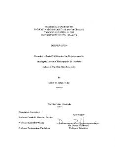
to the floor diaphragms and can uplift from the foundation. As the SC-CBF columns are allowed to uplift at the base, the SC-CBF system has a rocking response under higher levels of lateral force, as shown in Figure 1.1(c). Thus, during seismic excitation, the total drift in an SC-CBF building consists of two components: drift due to rocking of the frame (rocking drift, δrocking) and drift due to deformation in SC-CBF itself (frame drift, δframe) as shown in Figure 1.1(d). Note that the rocking drift does not cause damage in the SC-CBF members, as it is a rigid-body rotation about the base. The SC-CBF also includes lateralload bearings shown in Figure 1.1(b), located between the SC-CBF columns and the adjacent gravity columns at each floor level. These bearings transmit lateral inertia forces from the floor diaphragms to the SC-CBF while allowing relative vertical displacement between the adjacent gravity columns and SC-CBF columns (Roke et al. 2010). The lateralload bearings are designed to dissipate energy through friction during seismic excitation. Additionally, the vertically oriented post-tensioning (PT) bars in the SC-CBF as shown in Figure 1.1(b) are used in combination with gravity loads to produce restoring force in order to resist column uplift and provide self-centering (i.e., to reduce residual drift). There are several other types of self-centering frames with similar behavior that has been investigated by Blebo & Roke (2015) and Rahgozar et al. (2016) that is not considered in this study. Figure 1.2 shows typical CBF and SC-CBF lateral force-displacement behavior. Compared with the CBF behavior, the rocking behavior in the SC-CBF (after SC-CBF column decompression and before PT bar yielding) softens the lateral force-displacement response of the system, thereby permitting larger lateral displacements (prior to yielding or buckling in the braces) without increasing the force demand in the system. Thus the drift capacity in the SC-CBF prior to member yielding is increased, as indicated in Figure 1.2.
2
Recent experimental research (Roke et al. 2009, 2010) has shown that SC-CBFs can maintain the stiffness of conventional CBF systems while significantly reducing the probability of structural damage and eliminating residual drift under the design-basis earthquake for a 4-story SC-CBF structure subjected to design basis earthquake (DBE). However, seismic performance of the SC-CBF has not been evaluated for other levels of the ground motion hazard such as frequently occurring earthquake (FOE) and maximum considerable earthquake (MCE) and for other prototype structures (i.e., other configurations). Moreover, performance of non-structural components in SC-CBF system has not been assessed. Seismic performance of non-structural components is very important because buildings that suffer limited or no structural damage may exhibit extensive damage of non-structural components, which may result in serious economic loss and impede building operation (Lagorio 1990, Vergas & Bruneau 2007, Peiravian et al. 2014). Furthermore, in many strong earthquakes in the twentieth century in the US, the cost of damages to non-structural components has exceeded the cost of structural damage for most affected buildings (Filiatrault et al. 2001). Despite the better seismic performance of SC-CBF system, the construction cost of an SC-CBF is expected to be greater than that of a conventional CBF due to the special details and elements required by the SC-CBF. Therefore, stakeholders would be attracted to utilize SC-CBF system if the higher construction cost of SC-CBF system would be paid back by lower losses in earthquakes (due to better seismic performance of SC-CBF) during life cycle of the building. To demonstrate the effectiveness (i.e., better performance and economic feasibility) of SC-CBF systems, a more comprehensive study is needed to evaluate the benefit of using
3
an SC-CBF system instead of a conventional CBF system: (1) more prototype structures should be considered (particularly buildings with higher number of stories); (2) the seismic performance of SC-CBF systems should be evaluated considering all levels of seismic hazards including maximum considerable earthquake (MCE) and frequently occurring earthquake (FOE), compared with that of conventional CBF systems; and (3) the seismic performance of non-structural components in buildings with SC-CBF system need to be considered as well, (4) economic feasibility of the SC-CBF needs to be evaluated. This study conducts a performance evaluation and economic feasibility study on the SC-CBF and CBF systems. Performance evaluation study will complement the current knowledge about seismic response and performance of the SC-CBF system especially in taller buildings. In particular, the seismic responses are obtained through the numerical modeling of three configurations of CBF and SC-CBF (6- , 8- and 10- story buildings, representing mid-rise and high-rise buildings, respectively) subjected to a group of ground motion records. The probabilistic models for engineering demand parameters (EDP) (e.g., inter-story drift and peak floor acceleration) will be developed. Then, the structural and non-structural performance of the SC-CBF and the CBF systems will be evaluated using seismic fragility and engineering demand hazard curves. The results of performance evaluation will be further used in economic feasibility study. The aim of the economic feasibility study is to help stakeholders and decision makers learn about the benefits of using the SC-CBF system instead of CBF considering the location, occupancy, and configuration of their buildings. Using life cycle cost assessment, the proposed framework estimate the break-even (or pay-off) time during the lifetime of the structure with SC-CBF system, as the SC-CBF has a higher initial
4
construction cost but better seismic performance and lower earthquake induced losses compared with the CBF. The results of the economic feasibility are expected to vary with different configuration, locations and occupancy types of the buildings. 2. Objectives of This Dissertation The goal of the proposed work is to demonstrate the economic feasibility of the SC-CBF compared with the conventional CBF. The hypothesis is that even though the SC-CBF has a higher initial construction cost, the SC-CBF is still beneficial through the time as it has better seismic performance that mitigates the earthquakes induced losses. The proposed work includes the following four objectives. Objective 1: Probabilistic seismic demand model development for the CBF and SCCBF Accurate probabilistic seismic demand models are essential in order to conduct seismic performance evaluation of the structures using seismic fragility and EDP hazard curves. The proposed demand models will fully consider all the relevant uncertainties associated with the EDPs in the CBF and SC-CBF systems due to seismic excitations. Such uncertainties include uncertainties in the ground motions, structural properties, model errors, and statistical uncertainties in the model parameters.
Objective 2: Performance evaluation of the CBF and SC-CBF SC-CBF system has been proved to indicate better structural performance than the CBF subjected to DBE excitations (Roke et al. 2010). To demonstrate the effectiveness of SCCBF systems, it is necessary to conduct a comparative study of the both structural and nonstructural seismic performance of SC-CBF systems with that of conventional CBF systems.
5
Such comparison is viable by developing fragility curves and EDP hazard curves using the probabilistic demand models developed in Objective 1. Objective 3: Life cycle cost assessment of the CBF and SC-CBF Life cycle cost of the buildings will include the initial construction cost, maintenance cost, and cost of damages due to earthquakes in the life cycle of the building. Life cycle cost assessment will demonstrate the benefits of SC-CBF through the time as it has better seismic performance that mitigates the earthquakes induced losses, even though the SCCBF has a higher initial construction cost. Objective 4: Parametric study on life cycle cost for various locations, occupancies and configurations Various building locations, occupancies and configurations are expected to affect the life cycle cost of the buildings. Therefore, a parametric study is needed to investigate the effectiveness of the SC-CBF considering locations, occupancies, and configurations. 3. Background and Technical Needs In this section background and technical needs of each objective is defined by reviewing the related literature and researches in this field and analytical tools that are necessary for each objective is presented. 3.1
Objective 1: Probabilistic Seismic Demand Model Development
For building systems, the EDPs, peak inter-story drift and residual inter-story drift, are usually used to measure structural damage and used to quantify the seismic performance of structures (Badpay & Arbabi 2008, Lin et al. 2010, Sabelli et al. 2003, Mayes et al. 2005, Wei et al. 2006, Uriz & Mahin 2008, Ruiz-García & Miranda 2010, Erochko et al. 2011, Song & Ellingwood 1999). However, other engineering demand parameters, such as 6
member forces, and member deformations, can also be used for structural damage quantification (e.g., Sharma et al. 2014). Peak floor acceleration and peak inter-story drift are also considered as measures of damage to non-structural components (e.g., Park & Ang 1985, Bachman et al. 2004, Vargas & Bruneau 2007, Karavasilis & Seo 2011) and can be used for non-structural seismic performance evaluation of a building system. Therefore, developing probabilistic demand models for the peak inter-story drift, residual drift, and peak floor acceleration are the first step for conducting the performance evaluation of CBF and SC-CBF. Various formulations for seismic demands have been proposed in previous research. For example, Choi et al. (2004) and Nielson & DesRoches (2007) used functions of peak ground acceleration (PGA) to predict seismic ductility and deformation demands for steel bridges. Lin et al. (2010) used a function of the ratio of spectral acceleration (Sa) at first period of the structure (T1) to Sa at 2T1 to predict peak inter-story drift for MRFs. Jeong et al. (2012) used functions of Sa to predict peak inter-story drift demand in multistory reinforced concrete buildings. Badpay & Arbabi (2008) used function of Sa to develop demand models of peak inter-story drift for CBFs and BRBFs. These formulations are based on linear regression with pre-selected intensity measures (IMs) such as PGA and Sa as predictors. These models are not always the most accurate model and/or sometimes they do not satisfy the assumptions of the regression. Therefore, a general procedure that can be used to build accurate unbiased probabilistic demand models is needed, in which it selects the best IMs as predictors and considers all the relevant uncertainties in the demand predictions.
7
To develop probabilistic seismic demand models, seismic responses of the structures to a candidate suite of ground motions need to be obtained. The selected ground motion records should capture a wide range of ground motion characteristics such as return period, intensity, frequency content, and duration to accurately capture randomness of the ground motions in the probabilistic demand models. Nielson & DesRoches (2007) used a suite of 96 synthetic ground motions that was specifically developed for the central and southeastern United States. Choi et al. (2004) used a suite of 100 synthetic ground motions developed by Hwang et al. (2001) for central and southeastern United States that are distributed probabilistically from weak to strong and includes uncertainty in the soil and seismic characteristics. Sabelli et al. (2003), Wei (2006), Lee & Foutch (2004) and Li & Ellingwood (2007) used parts of a suite of 140 ground motion records on FEMA SAC Steel Project (Somerville et al. 1997) on steel MRFs, which has been widely adopted in the fragility development of building systems in the literature. Thus, this suite of ground motions will be used in this study as well. Implication for current study: There is a need to develop accurate demand models of EDPs such as peak inter-story drift, residual drift, and peak floor acceleration in order to conduct the performance evaluations of the two systems. The probabilistic demand model development will examine the effectiveness of the IMs to the seismic responses of the CBF and the SC-CBF, considering all the relevant uncertainties, and assures the satisfaction of the assumptions in the linear regression. 3.2
Objective 2: Performance Evaluation of CBF and SC-CBF Systems
In the literature, various methods have been adopted to compare performance of different structural systems and infrastructures using various engineering demand parameters. For
8
example, Sajedi and Huang (2015 a,b) used maximum load bearing capacity and deflection for performance evaluation of corroded reinforced concrete beams. Sabelli et al. (2003) compared statistical characteristics of peak inter-story drifts of 3- and 6-story CBFs and buckling restrained braced frames (BRBFs) under seismic loading. Mayes et al. (2005) used maximum and average values of peak inter-story drift from a suite of 20 ground motions to compare performance of 3- and 9-story buildings with four different steel structural systems (moment resisting frame (MRF), BRBF, viscous damped moment frame, and base isolated conventional braced frame). Badpay & Arbabi (2008) used seismic fragility curves of inter-story drifts to compare performance of CBFs and BRBFs. Lin et al. (2010) used peak inter-story drift hazard curves to compare seismic performance of 6- and 20-story eccentrically braced frames, BRBFs, and MRFs. Erochko et al. (2011) used mean values of peak inter-story drifts and residual drifts responses to a suite of 40 ground motions to compare performance of 6- and 10-story special MRFs and BRBFs. Dyanati & Huang (2014a) investigated collapse fragility of a fixed offshore platform under seismic loading using base shear demand and capacity considering impacts of various load patterns of push over analysis on the seismic fragility evaluation. Among the tools that are used by other researchers, seismic fragility and engineering demand hazard curves are better tools for performance evaluation because they can account for prevailing uncertainties and can also be easily extended for damage and loss analyses. Seismic fragility is defined as the conditional probability that an engineering demand parameter (e.g., peak inter-story drift, residual inter-story drift and peak floor acceleration) attains or exceeds a specified capacity level conditioned on seismic intensity measures (IMs). Seismic fragility provides a useful comparison of seismic performance of
9
different structures when the structures are subjected to the same IM level regardless of site. Seismic hazard of an engineering demand parameter, on the other hand, is defined as the mean annual rate of exceedance of a specified demand quantity, integrating the seismic fragility curve and the mean annual rate of exceeding the IM level at the site of the structure. Seismic hazard of demand becomes particularly useful when seismic fragilities are conditioned on different IMs and direct comparison of fragilities becomes impossible. Additionally, if the conditioned IM used in the seismic fragility depends on structural properties (e.g., spectral acceleration, Sa) (i.e., the mean annual rates of exceedance of these IMs can be different for structures with different structural properties in the same site), equal fragilities at a given IM do not necessarily indicate the same seismic performance of the structures. Thus, the demand seismic hazard that incorporates site effects and structural properties becomes necessary. Therefore, both seismic fragilities and seismic hazard curves are useful to compare seismic performance of CBF and SC-CBF structures. Implication for current study: Seismic fragility and seismic hazard curves are needed to be developed for the CBF and SC-CBF for the seismic performance evaluation. Seismic fragility and seismic hazard curves can also further be used in the loss analysis of the economic feasibility study conducted next. 3.3
Objective 3: Life-cycle Cost Assessment of CBF and SC-CBF Systems
Life cycle cost assessment has been used as a measure of the economic effectiveness of a structure. Wen & Ang (1991) and Wen & Shinozuka (1994, 1998) developed a life cycle cost formulation to investigate the cost effectiveness of an active control system in structures during earthquakes. Goda et al. (2010) used life cycle cost assessment to investigate the cost-effectiveness of a seismic isolation technology. Kang & Wen (2000)
10
used minimum life cycle cost concept to develop an optimal design for structures under single and multiple hazards. Cha & Elingwood (2013) used the life cycle cost of buildings considering wind hazards to develop a methodology to quantify various attitudes towards hazard risk (risk taking, risk neutral and risk adverse). Padgett et al. (2009) developed a retrofit strategy for bridges based on cost-benefit analysis using life-cycle cost to determine the most cost-effective retrofit method that differs based on the seismic hazard characteristics of the location. Life cycle cost of a building system subjected to seismic hazard includes three components (Kang & Wen 2000): construction cost, earthquake induced losses, and operation/maintenance cost during the life cycle of the building, as shown below. LCC t, x C0 x LCL t, x Cm x
(1.1)
where LCC = life cycle cost of the building; t = life time of the building; x = vector of design variables for building; C0 = initial construction cost of the building (including structural and non-structural components cost); LCL = life cycle loss of the building, the losses due to the earthquake induced consequences (e.g., repair cost, business interruption, injuries); and Cm = operation/maintenance cost of the building. Construction cost estimation is straightforward and can be generally estimated using expert’s opinion or tools such as R.S. Means Building Construction Cost Data (RS Means 2013a). Maintenance and operation costs are highly related to the occupancy of the building rather than structural system and can be estimated using handbooks and standards such as Facilities Maintenance & Repair Cost Data Online (RS Means 2013b). The life cycle loss estimation, on the other hand, usually involves more complex procedures and when seismic hazard is considered, it consists of four general steps (Baker & Cornell 2008):
11
1) determining earthquake occurrence and intensities (hazard analysis), 2) evaluating the responses of the building to earthquake (structural analysis), 3) determining damage states (damage analysis), and 4) determining costs/losses due to the damage (loss analysis). Each step involves both inherent (aleatory) randomness and (epistemic) model uncertainty that should be accounted for appropriately. 3.3.1
Hazard Analysis
Hazards are usually considered by assuming past events as scenarios (e.g., Kermanshah et al 2014) or assuming stochastic process for occurrence of the event in time (Kang & Wen 2000). In terms of seismic hazard consideration, there are scenario based hazard consideration/loss estimation and time based hazard consideration/loss estimation methods. Scenario-based loss estimation calculates the consequences and losses based on one scenario or multiple scenarios of earthquake (e.g., Gunturi & Shah 1993, Erberik & Elnashai 2006, Kermanshah et al 2014), and is usually used in regional loss estimation that calculates losses for a group of buildings in a region subjected to (a) specific scenario earthquake(s) (e.g., Algermissen et al. 1972, Erberik & Elnashai 2006, DeBock et al. 2013). However, the computation can be expensive if the scenario-based loss estimation is used for life cycle cost estimation, as it needs to consider all the possible earthquake scenarios that occur during the life time of the building. Time-based loss estimation considers earthquake scenarios that occur through the life cycle of the building by modeling the earthquake occurrence as a stochastic process, and Poisson process is usually adopted (e.g., Kang & Wen 2000, Padgett et al. 2009). Poison process is a memory-less process and assumes that the buildings are restored to the initial undamaged condition after each earthquake occurrence. Other stochastic processes
12
(e.g., Markov process) have been used as well in order to consider the degradation of structural strength due to aging or earthquake-induced damages (e.g., Anagnos & Kiremidjian 1984, Takahashi et al. 2004). 3.3.2
Structural Analysis
Responses of the buildings to earthquakes contain inherent uncertainty because of the record-to-record variability, material properties variability, and geometrical uncertainties. Such probabilistic nature of the building responses to ground motion in loss estimation formulations are usually considered by developing probabilistic EDP models (e.g., Ellingwood & Wen 2005, Kang & Wen 2000) or using Monte Carlo simulations over various ground motion records and other sources of uncertainties such as structural properties (e.g., Singhal & Kiremidjian 1996, Porter & Kiremidjian 2001). 3.3.3
Damage and Loss Analysis
Damage states are usually described qualitatively, and then defined by considering limit states on the EDPs (i.e., EDP capacities). Corresponding losses for each damage state are evaluated based on the description of the damage state. Damage and loss analysis of a building can be performed using approaches that are component-based, assembly-based (i.e., group of components), story-based, and building-based. The difference among these approaches lies in the levels of the damage definition (limit states) and the corresponding loss evaluation. In the component-based and assembly-based approaches, the damage states and the corresponding loss values are defined for each individual (or assemblies of) structural and non-structural components (e.g., beams, columns, ceilings, windows) in the building. The total loss of the building will be the sum of the losses calculated for each component (or assemblies of the components). On the other hand, in the story-based and
13
building-based approaches, the damage states are defined and the loss values are estimated for each story as a whole and for the whole building, respectively. The damage states and corresponding loss values can be found in codes and guidelines (e.g., ATC 1985, FEMA227&228 1992, FEMA-P58 2012) or in other studies on performance and loss evaluation of the buildings (e.g., Ramirez & Miranda 2009, Bai et al. 2009). If EDPs are used for quantifying the damage states, then those EDPs (or capacities) will be defined accordingly based on those levels. Scholl et al. (1982) developed a probabilistic component-based damage and loss evaluation method to study three example buildings considering 1971 San Fernando earthquake, where the component damage functions (i.e., component fragility functions) are generated based on experimental data. Park & Ang (1985) used the story-based damage and loss evaluation for several reinforced concrete moment resisting frame buildings. Kang & Wen (2000) used building-based damage and loss evaluation to calculate minimum life cycle cost of concrete building for design optimization purposes. Porter & Kiremidjian (2001) introduced assembly-based vulnerability, a fully probabilistic performance evaluation framework that incorporates the uncertainty propagation from the building damage estimates and the associated repair costs, and a three-story office building in Los Angeles was studied. Williams et al. (2009) applied the building-based damage and loss evaluation to a decision making process on retrofit of two identical two-story reinforced concrete frame buildings that represents low-rise constructions typically found in MidAmerica. Zareian & Krawinkler (2009) used grouping of the components into subsystems (in one story or in total building) for damage and loss analysis in order to develop a simplified approach towards performance-based earthquake engineering.
14
3.3.4
Life-cycle Loss Formulation
Life cycle loss, LCC, in Eq. (1.1) should be treated as a random variable since its estimation involves many sources of uncertainties. The expected value of life cycle loss, E[LCC], can be calculated using the following formulation (Kang & Wen 2000), N t k E LCL t , x E C j e ti Pij x, ti i 1 j 1
(1.2)
where i = number of seismic loading occurrences; N(t) = total number of seismic loading occurrences in t; j = number of limit state, k = total number of limit states under consideration; Cj = cost in present dollar value of the jth limit state being reached; e-γti = discounted factor over the time ti, γ = constant discount rate per year; Pij = probability of the jth limit states being exceeded given the ith occurrence of seismic loading; ti = occurrence time of the ith seismic loading. Note that the discount rate is used to calculate the value of losses that will occur in the future based on the present value. Higher discount rate indicates the lower present value of the future loss and vise versa. According to FEMA227 (1992), for public sector and private sector considerations, a discount rate of 3% to 4% and 4% to 6% are suggested respectively. If the earthquake occurrence is assumed as a Poisson Process with an occurrence rate of λ per year and multiple discrete damage states are considered, Eq. (1.2) can be evaluated in a closed form as shown below (Kang & Wen 2000), E[ LCL t , x ]
k 1 e t C j Pj j 1
(1.3)
Note that if non-Poisson processes is used for modeling earthquake occurrence, Monte Carlo simulations is usually applied because no explicit formulation has been derived. Since the damage states can be identified by limit state exceedance, based on loss analysis
15
conducted by Kang & Wen (2000) and Porter et al. (2004), Eq. (1.3) can be rewritten as follows: E[ LCL t , x ]
1 e t EAL
(1.4)
k
EAL C j ln 1 Pa, j ln 1 Pa, j1
(1.5)
j1
where EAL = expected annual loss, Pa,j = annual probability of exceeding the jth limit state. As mentioned earlier, exceeding limit states are normally defined by exceeding certain values of EDPs (EDP capacities) during ground motions (e.g., ASCE-41 2007). Usually the EDP capacities are treated deterministically in the literature, thus Pa,j = Pa(EDP > EDPc,j), where Pa(·) = annual probability, EDPc,j = capacity for EDP of interest for jth limit state, and Pa,j can be obtained from EDP hazard curves. However, if the variability in the capacities needs to be considered, EDP hazard curves cannot be used directly. 3.3.5
PEER Loss Estimation Methodology
While Eq. (1.5) can be used to compute the EAL, there is another alternative approach, the Pacific earthquake engineering research center (PEER) loss estimation methodology. PEER methodology for the loss estimation is a component-based methodology that applies the total probability theorem to evaluate the mean annual rate of exceeding for a decision variable (e.g., repair cost, repair time, human fatalities). The original formulation of this methodology was developed by Cornell & Krawinkler (2000) and has been improved by many other PEER researchers (e.g., Aslani & Miranda 2005, Mitrani-Reiser 2007, Ramirez & Miranda 2009), Methods for uncertainty propagation in PEER methodology have been investigated by Baker & Cornell (2008).
16
The mathematical formulation of PEER methodology is presented below (Ramirez & Miranda 2009)
DV
G DV DM dG DM EDP dG EDP IM d IM
(1.6)
where DV= decision variable(s); λ(DV) = mean annual rate of exceeding specific values of DV; DM = damage measures (or damage states); G(x|y) = complementary cumulative distribution function of x conditioned on y; and λ(IM) = mean annual occurrence rate of a specific IM. PEER loss estimation methodology transfers the hazard functions of earthquake intensity, λ(IM) , to hazard functions of decision variables, λ(DV), through four stages of hazard analysis, structural analysis, damage analysis, and loss analysis. Considering monetary losses, ML, as the decision variable in Eq. (1.6), EAL in Eq. (1.4) can be calculated as follows:
d ML EAL EML E d ML 3.3.6
(1.7)
Comparison of Loss Estimation Formulations
As described above, there are two ways for EAL estimate for Eq. (1.4): Eq. (1.5) (called LCL formulation) and Eq. (1.7) (called PEER formulation). Both formulations have their own advantages and drawbacks. The PEER formulation can fully incorporate the relevant uncertainties in the four stages but needs the evaluations of the complementary cumulative distribution functions (shown in Eq.( 1.6)), which is rather complicated (usually Monte Carlo simulation is needed). It is usually adopted for the loss estimation of a specific building with particularly designed components (e.g., Zareian & Krawinkler 2009, Ramirez & Miranda 2009), and it can provide accurate loss estimation by evaluating the loss evaluation of each component of the building. However, this accuracy is only
17
achievable when the following information is available: accurate fragilities, loss functions for each specific component of the building, and correlation of the losses for various components in order to prevent replicates in the loss evaluation (e.g., repairing damaged beams and columns needs demolishing and replacing of ceilings). The LCL formulation does not consider the uncertainties in the damage states and the corresponding loss values, but it can be applied to general loss analysis that can be component-based, assembly-based (i.e., group of components), story-based, and buildingbased. More importantly, the LCL formulation can be evaluated using a closed form, which is computationally efficient. Particularly, the LCL formulation has been used by many researchers for comparative studies (i.e., no specific detail design is required), such as comparing several retrofit strategies (e.g., Padgett et al. 2009, Williams et al. 2009) or investigating the cost benefits of new systems in buildings that mitigate earthquake induced losses (e.g., Wen & Ang 1991, Wen & Shinozuka 1994). 3.3.7
Loss Estimation Existing Software Packages
Several loss estimation tools have been developed and used to conduct damage and loss analysis of buildings. The Federal Emergency Management Agency (FEMA) and the National Institute of Building Sciences (NIBS) developed a GIS-based regional loss estimation methodology and a corresponding software named HAZUS (NIBS 1997) for loss assessment due to various types of hazards (e.g., seismic hazard, flood hazard, hurricanes hazard). This software includes an inventory of fragilities and loss functions for various types of buildings. However, these fragilities are predefined and the demand models used are defined as functions of only one specific IM, Sa. Although HAZUS is developed and used for regional loss evaluation (e.g., Erberik & Elnashai 2006, Tantala et
18
al. 2008), it also has been improved to calculate building specific loss by a new module named Advanced Engineering Building Module (Kircher et al. 2006). Another loss estimation tool called PACT is developed in FEMA-P58 (2012) based on the PEER methodology, and it has been used in the recent studies (e.g., DeBock et al. 2013, Parvini Sani & Banazadeh 2012). It includes fragilities and loss functions for structural and non-structural components for many types of building. The direct and indirect losses of a specific building can be calculated for scenario-based loss estimation and/or time-based loss estimation considering the hazards of ground motion at the building location. The inputs consist of a detailed list of structural and non-structural components of the building, population schedule of the building, and the response characteristics of the structure for selected ground motions. These responses are used in the software to develop EDP models defined as functions of Sa. PACT also considers the losses due to collapse and the possibility of demolishing the structure due to high residual drifts. Although both HAZUS and PACT have been used in the seismic performance and loss evaluation of buildings, there are some drawbacks. Both HAZUS and PACT use EDP models defined as a function of Sa only that may not be an accurate EDP model for the building studied (Dyanati et al. 2014b), which eventually will lead to inaccuracy in the loss evaluation. Furthermore, in HAZUS, the fragility functions for defining damage states of buildings need to be updated according to the state-of-the-art knowledge in this field (Ramirez & Miranda 2009), resulting in over/under-estimate of the losses. Although PACT, as newly developed software, has fragilities based on the state-of-the-art knowledge, it requires accurate definitions of building components and the correlation
19
between damage states of different components. Therefore, it is only practical if that information is available. Implication for current study: Life cycle cost for both frame types (SC-CBF and CBF) is needed to be evaluated, and the LCC formulation is suitable for the proposed work. However, the uncertainties in damage states and corresponding loss values of each damage state should be incorporated into the current LCC formulation. 3.4
Objective 4: Parametric Study on Life-cycle Cost for Various Locations, Occupancies, and Configurations
Loss estimation of the buildings depends on the locations, configuration, and occupancies of the buildings. Different locations lead to different hazards of seismic IMs, the configuration of the building will affect its response to ground motions, and occupancy of the building, determines the type of non-structural components, population of residents, and the contents of the buildings, which in turn affect the initial construction cost and earthquake induced losses of the buildings due to hazards. Therefore, for a comprehensive economic feasibility study of SC-CBF, several configurations and occupancies of the buildings at various locations will be included in the study. Implication for current study: LCC must be calculated for several configuration and occupancies of the buildings in order to perform a comprehensive comparative study for CBF and SC-CBF systems. 4. Dissertation Outline In Chapter I, Backgrounds and objectives of this study is elaborated. In Chapter II, probabilistic demand model development process is introduced and corresponding probabilistic inter-story drift and residual drift demand models are developed for a 20
prototype 6-story building in downtown Los Angeles with exclusively CBF and exclusively SC-CBF configurations. The developed probabilistic demand models are used to evaluates seismic performance of prototype buildings and compare seismic performance of SC-CBF and CBF systems as using seismic fragility and engineering demand hazard curves. In Chapter III, same methodology of chapter 2 is used for probabilistic demand model development for inter-story drift and floor accelerations for same prototype buildings. Then, structural and non-structural performance of SC-CBF and CBF systems are compared. In Chapter IV, developed damage analysis, loss analysis, life cycle loss analysis and economic benefit calculation methodologies are defined. These methodologies are utilized to calculate annual probabilities of exceeding various damage states and expected annual loss for SC-CBF and CBF systems in 6-story and 10-story configurations located in downtown Los Angeles. Moreover, economic benefit of using SC-CBF system instead of a CBF system evaluated for the prototype buildings. In Chapter V, the proposed methodology of damage, loss and economic benefit analysis is applied to more case studies in order to perform a comprehensive study on performance and economic benefit of SCCBF system. Particularly, the damage, loss and economic benefit analysis methodologies is utilized for 6-, 8-, and 10-story buildings located in downtown Seattle and downtown Los Angeles. Moreover, two different suites of ground motions are used to develop demand models that are utilized in the damage, loss and economic benefit analysis methodologies. Furthermore, three occupancies of office buildings/ banks and financial institutions and retail trades are considered for economic benefit analysis of SC-CBFs. Finally, Chapter VI represents the conclusions of this study.
21
Manuscript has been submitted and published in Engineering Structures, Proceedings of Structures Congress 2014, Journal of Structures and Infrastructure Engineering based on the materials in Chapter II, Chapter III, and Chapter IV of this dissertation, respectively.
22
(a) (b) (c) (d) Figure 1.1. (a) Configuration of CBF; (b) configuration of SC-CBF; (c) rocking behavior of SC-CBF; (d) drifts in the SC-CBF
Figure 1.2. SC-CBF and CBF idealized schematic of lateral force-drift behavior
23
CHAPTER II
DEMAND MODELS DEVELOPMENT AND STRUCTURAL PERFROMNACE EVALUATION
1. Introduction
While conventional concentrically braced frames (CBFs) have been widely used as earthquake resistant structural systems, they suffer from limited drift capacity and high residual drift, leading to expensive post-earthquake costs. Extensive damages in CBFs have been reported after many recent earthquakes, including the 1985 Mexico City (e.g., Osteraas & Krawinkler 1985), 1989 Loma Prieta (e.g., Kim 1992), 1994 Northridge (e.g., Tremblay et al. 1995; Krawinkler et al. 1996), and 1995 Hyogo-ken Nanbu (e.g., Tremblay et al. 1996, Steel Committee of Kinki Branch 1995, Hisatoku 1995) earthquakes. To address the limitations of conventional CBFs, damage-free self-centering CBFs (SC-CBFs) have been developed (Roke et al. 2006) to increase the drift capacity of the structure prior to damage and to reduce residual drift. Figures 2.1(a) and 2.1(b) show the general configurations of a CBF and an SC-CBF, respectively. Different from the CBF, the SC-CBF has two types of columns as indicated in Figure 2.1(b): adjacent gravity columns
24
and SC-CBF columns. Adjacent gravity columns are connected to the floor diaphragms and do not uplift from the foundation, while SC-CBF columns are not directly connected to the floor diaphragms and can uplift from the foundation. As the SC-CBF columns are allowed to uplift at the base, the SC-CBF system has a rocking response under higher levels of lateral force, as shown in Figure 2.1(c). Thus, during seismic excitation, the total drift in an SC-CBF building consists of two components: drift due to rocking of the frame (rocking drift, δrocking) and drift due to deformation in SC-CBF itself (frame drift, δframe) as shown in Figure 2.1(d). Note that the rocking drift does not cause damage in the SC-CBF members, as it is a rigid-body rotation about the base. The SC-CBF also includes lateralload bearings shown in Figure 2.1(b), located between the SC-CBF columns and the adjacent gravity columns at each floor level. These bearings transmit lateral inertia forces from the floor diaphragms to the SC-CBF while allowing relative vertical displacement between the adjacent gravity columns and SC-CBF columns (Roke et al. 2010). The lateralload bearings are designed to dissipate energy through friction during seismic excitation. Additionally, the SC-CBF has vertically oriented post-tensioning (PT) bars as shown in Figure 2.1(b), which are used in combination with gravity loads to produce restoring force in order to resist column uplift and provide self-centering (i.e., to reduce residual drift). Figure 2.2 shows typical CBF and SC-CBF lateral force-displacement behavior. Compared with the CBF behavior, the rocking behavior in the SC-CBF (after SC-CBF column decompression and before PT bar yielding) softens the lateral force-displacement response of the system, thereby permitting larger lateral displacements (prior to yielding
25
or buckling in the braces) without increasing the force demand in the system. Thus the drift capacity in the SC-CBF prior to member yielding is increased, as indicated in Figure 2.2. Recent experimental research (Roke et al. 2009, 2010) has shown that SC-CBFs can maintain the stiffness of conventional CBF systems while significantly reducing the probability of structural damage and eliminating residual drift under the design-basis earthquake. However, to demonstrate the effectiveness of SC-CBF systems, it is necessary to conduct a comparative study of the seismic performance of SC-CBF systems with that of conventional CBF systems. For building systems, the engineering demand parameters, peak inter-story drift and residual inter-story drift, are usually used to measure structural damage and used to quantify the seismic performance of structures (Erochko et al. 2011, Lin et al. 2010, Ruiz-García & Miranda 2010, Badpay & Arbabi 2008, Uriz & Mahin 2008, Wei 2006, Mayes et al. 2005, Sabelli et al. 2003, Song & Ellingwood 1999). However, other engineering demand parameters, such as floor acceleration, member forces, and member deformations, can also be used for structural and non-structural damage quantification (e.g., Sharma et al. 2014, Dyanati et al. 2014b). In the literature, various methods have been adopted to compare seismic performance of different structural systems using various engineering demand parameters. For example, Sabelli et al. (2003) compared statistical characteristics of peak inter-story drifts of 3- and 6-story CBFs and buckling restrained braced frames (BRBFs) under seismic loading. Mayes et al. (2005) used maximum and average values of peak inter-story drift from a suite of 20 ground motions to compare performance of 3- and 9-story buildings with four different steel structural systems (moment resisting frame (MRF), BRBF, viscous damped moment frame, and base isolated conventional braced frame). Badpay and Arbabi
26
(2008) used seismic fragility curves of inter-story drifts to compare performance of CBFs and BRBFs. Lin et al. (2010) used peak inter-story drift hazard curves to compare seismic performance of 6- and 20-story eccentrically braced frames, BRBFs, and MRFs. Erochko et al. (18) used mean values of peak inter-story drifts and residual drifts responses to a suite of 40 ground motions to compare performance of 6- and 10-story special MRFs and BRBFs. In this study, seismic fragility and seismic hazard curves for engineering demand parameters (peak inter-story drift and residual inter-story drift) will be used to describe the seismic performance of CBF and SC-CBF systems. Seismic fragility and engineering demand hazard curves account for prevailing uncertainties and can also be easily extended for damage and loss analyses. Seismic fragility is defined as the conditional probability that an engineering demand parameter (in this study, peak inter-story drift and residual inter-story drift) attains or exceeds a specified capacity level conditioned on seismic intensity measures (IMs). ASCE 41-06 (2007) specifies inter-story and residual inter-story drift capacities to define three performance levels of steel structures: immediate occupancy (IO), life safety (LS), and collapse prevention (CP). Seismic fragility provides a useful comparison of seismic performance of different structures when the structures are subjected to the same IM level regardless of site. Seismic hazard of an engineering demand parameter, on the other hand, is defined as the mean annual rate of exceedance of a specified demand quantity, integrating the seismic fragility curve and the mean annual rate of exceeding the IM level at the site of the structure. Seismic hazard of demand becomes particularly useful when seismic fragilities are conditioned on different IMs and direct comparison of fragilities becomes impossible. Additionally, if the conditioned IM used in the seismic fragility
27
depends on structural properties (e.g., spectral acceleration, Sa) (i.e., the mean annual rates of exceedance of these IMs can be different for structures with different structural properties in the same site), equal fragilities at a given IM do not necessarily indicate the same seismic performance of the structures. Thus, the demand seismic hazard that incorporates site effects and structural properties becomes necessary. Therefore, in this study, both seismic fragilities and seismic hazards for peak inter-story drift and residual inter-story drift are developed to compare seismic performance of CBF and SC-CBF structures. Probabilistic demand models are necessary to assess seismic fragility and seismic hazard for engineering demand parameters. Various formulations for seismic demands have been proposed in previous research. For example, Choi et al. (2004) and Nielson & DesRoches (2007) used functions of peak ground acceleration (PGA) to predict seismic ductility and deformation demands for steel bridges. Lin et al. (2010) used a function of the ratio of spectral acceleration (Sa) at first period of the structure (T1) to Sa at 2T1 to predict peak inter-story drift for MRFs. Jeong et al. (2012) used functions of Sa to predict peak inter-story drift demand in multi-story reinforced concrete buildings. Badpay and Arbabi (2008) used function of Sa to develop demand models of peak inter-story drift for CBFs and BRBFs. This study adopt a probabilistic formulation following Huang et al. (2010), where the probabilistic demand model consists of a deterministic demand prediction used in practice, correction terms, and model errors. The use of a deterministic demand model is to facilitate the practical application of the probabilistic demand models. The purpose of the correction terms is to correct the bias and improve the prediction accuracy of the selected deterministic demand. The model parameters are assessed using
28
the seismic responses obtained from nonlinear dynamic analyses performed on finite element models (FEMs) of a prototype structure subjected to a suite of ground motion records. In this study, a six-story prototype office building is designed using exclusively CBFs and exclusively SC-CBFs as the lateral-load-resisting system, respectively. The proposed demand models will account for the uncertainties from ground motions, model parameters, material properties, and model errors. Based on the capacities defined by ASCE 41-06 (2007) and the probabilistic demand models, fragility curves for three performance levels (IO, LS, and CP) are developed. The comparison of the fragility curves can indicate which system is more likely to reach or exceed a performance level for given ground motion IMs. Also, using the probabilistic demand models, peak inter-story drift and residual inter-story drift demand hazard curves are developed. The demand hazard curves are used to compare the performance of CBF and SC-CBF considering the IM hazards at the site of the structures. Moreover, the impact on the engineering demand hazard curves of probabilistic demand models using various formulations is also investigated. 2. Numerical Analysis In this section, the designs of the prototype structures that are used for the comparison study are presented. Then, the nonlinear numerical analysis of the prototype structures is described, including the modeling details, ground motion selection, and numerical analysis results. Those numerical analysis results will be further used for the development of probabilistic demand models.
29
2.1
Prototype Structure
In order to conduct a comparative study of the seismic performance of SC-CBF and CBF systems, two six-story prototype office-building structures with identical configurations are designed using exclusively CBFs and exclusively SC-CBFs as the lateral-load-resisting system, respectively. Each prototype building consists of six bays in each direction, as shown in the floor plan in Figure 2.3(a). A total of eight lateral-load-resisting frames (four in each direction) are designed for each building. Figures 2.3(b) and 2.3(c) show the CBF and SC-CBF frame elevation views, respectively. Both systems are designed for stiff soil as defined in ASCE 7-10 (2010) for a site in Los Angeles. The SC-CBF members are designed following the design procedure proposed by Roke et al. (2010). The CBF is designed as a special CBF, and its members are designed using the AISC specification (2010b) and seismic provisions (2010a) and the equivalent lateral force procedure in ASCE 7-10 (2010). Both frames’ members are further modified to satisfy the AISC seismic provisions (2010a). Table 2.1 shows the designed member sizes for the two systems. 2.2
Numerical Modeling
Numerical modeling of structures can be conducted using various software such as ANSYS (e.g., Sajedi et al. 2011), ABAQUS (e.g., Atashi et al. 2007), etc. In this study, the OpenSees platform (McKenna & Fenves 2000) is used to construct finite element models (FEMs) of the prototype structures and conduct nonlinear time history analyses with ground motion excitations. Columns, beams, and braces are modeled using bilinear isotropic hardening elastic-plastic materials (with 0.03 strain hardening ratio) and nonlinear beam-column elements with fiber cross-sections including P−Δ effects. A mid-
30
length node with out-of-straightness (equal to 1% of the member length) is added in each brace member to capture the possible buckling behavior, following the recommendations made by Uriz & Mahin (2008). However, no mid-length nodes are added to the columns and beams. Friction contact gap elements (Roke et al. 2010) are used to model the lateralload bearing elements in the SC-CBFs. These friction contact gap elements are capable of modeling gap behavior and transverse friction in the lateral-load bearing. The PT bars in the SC-CBF are modeled by a combination of different material models that allow the PT bar element to carry tensile forces with negligible bending and shear stiffness. In addition, a bilinear isotropic hardening elastic-plastic material (with 0.02 strain hardening ratio) is considered for the PT bars’ tensile strength. In the CBF model, brace and beam connections to columns are modeled as pin connections that transfer zero moment from the columns to the braces and beams, following the common practice in FEMs of CBFs. In the SC-CBF modeling, those connections are modeled to allow for moment transfer, following the SC-CBF design procedure (Roke et al. 2010). The foundation for both systems is modeled to be rigid, with the gravity columns (but not the SC-CBF columns) pinned to the ground. Inertia forces are applied based on the total mass of each floor (consistent with ASCE 7-10 2010 provisions) divided by the number of braced bays used in the building in each principal direction. Global P−Δ effects are also considered by adding vertical loads to the lean-on column based on the calculated dead and live loads of each floor on the prototype building. Additionally, Rayleigh damping of 2% in the first mode and 5% in the third mode are assumed, following common practice for dynamic analysis of steel structures. Note that the SC-CBF numerical modeling techniques utilized in this study have
31
been verified by Roke et al. (2010) through experimental tests conducted on a 4-story SCCBF test structure. 2.3
Ground Motions
To accurately capture randomness of the ground motions in the probabilistic demand models, selecting an appropriate suite of ground motion records for the numerical analysis is critical. The selected ground motion records should capture a wide range of ground motion characteristics such as return period, intensity, frequency content, and duration. This study adopts a set of 140 ground motion records used in the FEMA SAC Steel Project Somerville et al. (1997) on steel MRFs. This suite of ground motions consists of horizontal ground acceleration records designated for Los Angeles (LA), Seattle (SE), and Boston (BO), and has been widely used by other researchers in evaluating seismic performance of structures (e.g., ; Kafaeikivi et al. 2013, Uriz & Mahin 2008, Li & Ellingwood 2007, Lee & Foutch 2004, Sabelli & Mahin 2003). The ground motions are for stiff soil sites and are scaled by Somerville et al. (1997) to match the mean of the target response spectra defined in the NEHRP provisions. The earthquake records have hazard levels corresponding to 2% (for all three cities), 10% (for all three cities), and 50% (for LA only) probabilities of exceedance in 50 years. 2.4
Numerical Analysis Results
Figure 2.4 shows the typical roof drift responses of the SC-CBF and CBF under the LA31 and LA10 ground motions (Somerville et al. 1997), corresponding to 2% and 10% probability of exceedance in a 50-year period in Los Angeles, respectively. Peak roof drift responses for the SC-CBF are typically higher; however, as expected, the SC-CBF has lower residual drift, which is especially obvious for the ground motion with 2% probability 32
of exceedance in a 50-year period as shown in Figure 2.4(a). Additionally, due to friction energy dissipation, the dynamic response of the SC-CBF damps out much more quickly than the CBF response, which can lead to less structural and non-structural damage throughout the duration of the earthquake. The results shown in Figure 2.4 are typical for each ground motion record. In the CBF building, deformations in the gravity system and CBF are equal. Therefore, the inter-story drift in the gravity system is the same as the inter-story drift in the frame itself. On the other hand, because of the rocking behavior in the SC-CBF system, the deformations in the SC-CBF and gravity system are not equal. In other words, as shown previously in Figure 2.1(d), the drift of the gravity system (δtotal) is equal to summation of the rocking drift (δrocking, which will not result in any structural damages in the SC-CBF) and SC-CBF frame drift (δframe). Thus, for the SC-CBF structure, inter-story drifts must be calculated based on two considerations: δtotal for non-structural and gravity system damage, and δframe for SC-CBF member damage. The inter-story drifts based on δframe are negligible; therefore, to be conservative, the inter-story drift of the gravity system in the SC-CBF building is compared with the inter-story drift of the CBF building. Note that the interstory drift in SC-CBF building is mostly due to δrocking that does not cause structural damage in the SC-CBF members; therefore, different capacity limits for the inter-story drift should be applied for the CBF and SC-CBF systems, which will be discussed later. Examining the numerical analysis results, no PT bar fractures occurred during the ground motions, since the fracture strain was not exceeded. In addition, since the columns were not modeled to capture buckling behavior during the ground motions, the results from ground motions that caused peak force responses greater than the design buckling forces
33
in the columns (three ground motions for the CBF) are omitted from the result set in order to consider only valid results. Figure 2.5 shows the peak roof drift, peak inter-story drift, and residual inter-story drift responses and corresponding mean values for the CBF and the SC-CBF for three cities (LA, SE, and BO). Peak roof drift indicates the global response of the structure, while the peak inter-story drift and residual inter-story drift can be related to structural and non-structural damage. As shown in Figure 2.5, the CBF and the SC-CBF exhibit different peak roof drift, peak inter-story drift, and residual inter-story drift responses in LA and SE (having different mean values of the responses), while the mean response values for the two systems are similar in BO. The differences in the peak roof drift and peak inter-story drift mainly can be explained by the rocking behavior in the SCCBF: in BO with weaker ground motions, no or limited rocking behavior occurs and the two systems show similar responses; bigger differences in the structural responses are found in LA and SE because of the stronger ground motions in these two cities, which leads to more rocking behavior in the SC-CBF. The differences in the residual inter-story drift are mainly due to the self-centering of the SC-CBF. As shown in Figure 2.5(a), the maximum and mean values of SC-CBF peak roof drifts are higher than the CBF values. This is because of the reduced stiffness of the SCCBF after column decompression. As shown in Figure 2.5(b), the maximum and mean values of peak inter-story drifts for the SC-CBF are lower than those for the CBF. This is because opposing displacements in adjacent floor levels can cause large inter-story drifts in CBFs, while the rocking response of the SC-CBF forces all story drifts to be in same direction, reducing the inter-story drift demand. Additionally, as shown in Figure 2.5(c), the mean values of residual inter-story drifts in the SC-CBF are remarkably lower for most
34
ground motion records than the mean values of residual inter-story drifts in the CBF, indicating that the SC-CBF has less post-earthquake cost related to residual drift. However, several ground motions with a 2% exceedance in 50 years cause significantly high residual inter-story drifts in the SC-CBF; those data points are boxed in Figure 2.5(c). Different from the residual drift in the CBF, large residual drifts in the SC-CBF system are not caused by the damage in the structural members, but by the rocking of the SC-CBF and the loss of the restoring force from the PT bars. This loss of the restoring force is due to the excessive plastic deformation in the PT bar resulting from the high drift responses during the strong ground motions; thus, the restoring force provided by the PT bars is significantly reduced to a point where it is overcome by the P-Δ effect of the gravity system. If the PT bars do not fail, this type of residual drift can be easily reduced (or even eliminated) by re-tensioning the PT bars. Re-tensioning of the PT bars was simulated in numerical analyses conducted at the end of each ground motion record, resulting in a significant reduction in residual inter-story drifts for the SC-CBF (mean residual inter-story drift equal to 0.003%, 0.002%, and, 0.000% in LA, SE, and BO, respectively) as shown in Figure 2.5(c). To compare the numerical results of the two systems more clearly, the complementary cumulative distribution function (CCDF) of all responses for peak roof drift, peak inter-story drift and residual inter-story drift are constructed, as shown in Figure 2.6. The CCDF value refers to the percentage of the responses exceeding a specific value. In other words, if one system has higher CCDF values, that system has higher responses than the other system.
35
Similar to what is observed in Figure 2.5, Figure 2.6 shows higher values of peak roof drifts in the SC-CBF than the CBF, lower peak inter-story drifts in the SC-CBF than the CBF, and lower residual inter-story drift in the SC-CBF than CBF. Note that there are zero values of residual inter-story drifts for both systems; thus the CCDF values for residual inter-story drift start from about 70% and 10% for CBF and SC-CBF, respectively (as shown in Figure 2.6(c)), instead of 100% (as shown in Figures 2.6(a) and 2.6(b)). Additionally, for the residual inter-story drift, the CCDF curve of the SC-CBF is rather flat. This is because the uniqueness of the residual drifts of SC-CBF: 90% of the values are zeroes because of the self-centering feature and 10% are high residual drifts due to the excessive yielding of the PT bars. The high SC-CBF residual drifts, however, can be corrected by re-tensioning the PT bars. 3. Probabilistic Seismic Demand Model As mentioned earlier, peak inter-story drift and residual inter-story drift are typically used to measure structural and non-structural damage for building systems. This section develops probabilistic seismic demand models of peak inter-story drift and residual interstory drift for the CBF and the SC-CBF systems based on the numerical analysis results discussed in the last section. While advanced model development techniques such as Monte Carlo Markov Chain can be used to develop probabilistic demand models (e.g., Miran et al. 2016, Karduni et al 2016), linear regression is the most popular model development tool in civil engineering community (e.g., Rahmani et al. 2012, Kiani et al. 2012). Seismic demand models are usually formulated based on linear regression with pre-selected IMs (e.g., PGA, Sa) as predictors (e.g., Lin et al. 2010, Choi et al. 2004, Nielson & DesRoches 2004). In
36
this study, the probabilistic seismic demand model is developed following the formulation proposed by Huang et al. (2010), which consists of correction terms added to a deterministic demand prediction used in practice. The purpose of using the deterministic demand is to facilitate the practical application of our probabilistic model, while the use of the correction terms is to correct the bias and improve the prediction accuracy of the selected deterministic demand. The demand formulation is written as:
Dk (x, Θk ) dˆk (x) k (x, θk ) σ k
(2.1)
where Dk(x,Θk) = demand measure (or a suitable transformation such as natural logarithm);
dˆk (x) = demand or a suitable transformation predicted by a selected deterministic demand pk
model or procedure; γk(x,θk) = ki hi ( x ) = correction terms for correcting the bias and i 0
random errors in dˆk (x), in which hi(x) = explanatory functions (or a suitable transformation) and θk = (θk,0, …, θk,pk); Θk = (θk, σk) = a vector of unknown model parameters; pk+1 = number of the correction terms; σk = standard deviation of the model error; ε = normal random variable with zero mean and unit variance; x = vector of basic variables (e.g., material properties, member dimensions, and imposed boundary conditions); and k = the engineering demand parameter of interest (e.g., k = ID for peak inter-story drift and k = RD for residual inter-story drift). Two assumptions are used in the demand model in Eq. (2.1): the homoskedasticity assumption (i.e., σk is constant and independent of x) and the normality assumption (i.e., the model error has the normal distribution). Usually a variance stabilizing transformation of the demand quantities of interest can be used to satisfy both assumptions (Box & Cox 1964). Diagnostic plots can be used to check the suitability of the transformation (Sheather 2009, Rao 1997). This study adopts the natural logarithmic
37
transformation of the peak inter-story drift and residual inter-story drift demands. The following section discusses the selected deterministic demand models and the process of constructing the candidate correction terms. With the developed probabilistic demand model, seismic fragilities and engineering demand hazard curves for CBFs and SC-CBFs can be assessed. 3.1
Deterministic Demand Model
In this study, the deterministic demand for peak inter-story drift is calculated using the coefficient method (CM) presented in ASCE 41-06 (2007). This method is based on the response of an equivalent single-degree-of-freedom (SDOF) system that has a natural period equal to the first natural period of the multi-degree-of-freedom (MDOF) structure of interest. The maximum roof displacement of the structure is calculated using modification factors multiplied by the spectral displacement at first natural period of the structure. These modification factors are intended to account for impacts of the ground motion IMs, the structural system type, the relationship between the inelastic and the linear elastic displacement response of the structure, the effect of pinched hysteretic shape of the materials, cyclic stiffness degradation, and strength deterioration of the structure on the seismic displacement response. Additionally, the pseudo spectral acceleration at the structure’s first mode period (PSA) for each individual earthquake record is used to calculate maximum roof displacement. Finally, the deterministic demand model, dˆID(x) , in the probabilistic seismic demand model is determined by the peak roof drifts calculated based on the maximum roof displacements in the CM. There is no general formulation for predicting residual drift in practice, though some researchers proposed formulations for specific structures. For example, Ruiz-García
38
& Miranda (2010) proposed a probabilistic formulation for predicting residual inter-story drift and residual roof drift for 3-, 9- and 18-story generic frame buildings. This formulation uses a function of maximum inelastic displacement demand of an equivalent elastoplastic SDOF system with the same initial lateral stiffness as the building. Erochko et al. (2011) showed that residual inter-story drift of special MRFs and BRBFs can be estimated by multiplying a correction coefficient by the difference between the peak roof drift and the peak elastic roof drift (i.e., maximum drift before any member reaches yielding) of the structure. However, they found that their predictions are not accurate enough for the earthquakes with 2% probability of exceedance in 50 years. Overall, since there no prediction models for residual drift are available in practice and the prediction models available in the literature are developed for specific structures (but not for CBF or SC-CBF systems), no deterministic demand will be included in our probabilistic demand models for the residual inter-story drift. 3.2
Demand Model Development for Peak Inter-story Drift
As shown previously, the correction terms are γ(x,θ) =
pk
i 0
h ( x ) to remove the bias and
ki i
improve the accuracy of the deterministic demand model prediction. In order to detect a potential constant bias of the proposed model, one sets h0 (x) 1. To capture the under- or over-estimation of dˆ ID (x) , one sets h1 (x) dˆID (x) . Since the characteristics of ground motions are critical to determine the seismic responses of the structures (e.g., Jeong et al. 2012, Lin et al. 2010, Huang et al. 2010, Choi et al. 2004), IMs are used to construct potential explanatory functions. In this study, natural logarithms of the normalized IMs that are shown in Table 2.2 are used; these transformed functions are then used as h2(x) to
39
h13(x). In Table 2.2, T1 = natural frequency of the equivalent SDOF structure; Hc = total height of the structure; ug(t), u g (t ) , and ug (t ) denote the ground motion displacement, velocity, and acceleration at time t, respectively; Dt = duration of a ground motion record, and TD = t(0.95IA) − t(0.05IA) = strong ground motion duration based on the time between 2.5% and 97.5% of the Arias intensity IA (Trifunac et al. 1975). To make the proposed probabilistic demand model concise while maintaining the accuracy of the prediction, a model selection process is conducted to select explanatory functions that significantly statistically contribute to the model prediction. The full model size is 14 (pk = 13), with all the potential explanatory functions described above and indicated in Table 2.2. First, reduced models can be constructed with all possible combinations of the explanatory functions for each reduced model size (the reduced model size varies from 1 to 13). Then, the statistical significance of all of the reduced models and the statistical significance of their model parameters are checked by using F-test and extra sum of square test (Sheather 2009), respectively. Reduced models are discarded if the model has any pvalues obtained from F-test or extra sum of square test greater than 5%. Next, Akaike’s information criterion (AIC) (Sheather 2009) is used to select the two best models for each model size. To select the final model among all the best models, the number of the IMs in the candidate model and the standard deviation of the residuals of the model are used to measure the complexity of the model and accuracy of the model predictions, respectively. Thus, selection of the final model is a compromise between the model complexity and prediction accuracy. As a result of the model selection, the demand models of peak interstory drift are developed for both CBF and SC-CBF, as shown in the following equation:
40
PGV T1 ID DID (x, Θ ID ) ID 0 1 ID1 dˆID (x, PSA ) ID 2 log H c
(2.2)
The statistics of the model parameters are indicated in Table 2.3. Figures 2.7(a) and 2.7(b) show the comparison of the predicted values of peak interstory drifts from the deterministic model and the proposed demand model, respectively, with the numerical results obtained from FEM for the CBF. Figures 2.8(a) and 8(b) show the same comparison for the SC-CBF. The solid line has a slope equal to one and the dashed lines (in Figures 2.7(b) and 2.8(b)) show ±1 standard deviation band of the model error. For a perfect prediction, the data should lie along the solid line. As shown in Figures 2.7(a) and 2.8(a), the deterministic models tend to either underestimate or overestimate the peak inter-story drift demands. On the other hand, in Figures 2.7(b) and 2.8(b), the data points evenly spread around the solid line with most of the data falling within the dashed lines, indicating that the developed probabilistic demand models provide unbiased prediction; this relatively even spread of the data points about the solid line indicates that the standard deviation of the residuals remains constant (satisfying the homoscedasticity assumption). Furthermore, compared with Figures 2.7(a) and 2.8(a), the spread becomes smaller in Figures 2.7(b) and 2.8(b), implying that the developed probabilistic demand models provide better accuracy in predictions than the deterministic demand models. Note that in the literature (e.g., Jeong et al. 2012, Nielson & DesRoches 2007), two demand model formulations are widely adopted: linear regression models using natural logarithms of PGA and PSA as predictors, respectively. In order to compare the accuracy of our proposed probabilistic demand model with the models using the two mentioned widely adopted demand model formulations, two additional demand models are developed 41
(linear regression using log(PGA/g) and log(PSA/g), respectively) using the numerical results obtained in this study. Furthermore, the impact of the prediction accuracy of the demand model on the seismic performance evaluations of structures will be investigated. Table 2.4 gives the comparison of the demand models in terms of the satisfactions of normality and homoscedasticity assumptions and the accuracy of the model prediction (measured using standard deviation of model error and R squared). The normality and homoskedasticity assumptions are checked using diagnostic plots (Sheather 2009, Rao 1997). As indicated in Table 2.4, the proposed demand model gives higher values of R squared and lower standard deviations of model error compared to the other two models, implying better accuracy in our proposed probabilistic demand models. Furthermore, the demand models using log(PSA/g) do not satisfy the regression homoscedasticity assumption; thus, these models are not valid. Figures 2.7(c) and 2.7(d) shows the predictions of these two demand models vs. the numerical results obtained from FEMs for the CBF, and Figures 2.8(c) and 2.8(d) are for the SC-CBF. Consistent with the results shown in Table 2.4, for the CBF predictions, the spread of the data in Figure 2.7(b) is much smaller than Figures 2.7(c) and 2.7(d), indicating that the proposed probabilistic demand model gives better predictions than the state-of-thepractice prediction models. Similar observations are found for the SC-CBF as shown in Figures 2.8(b), 2.8(c), and 2.8(d). Also, Figures 2.7(c) and 2.8(c) show that the data points are not evenly spread about the ideal (not satisfying the homoscedasticity assumption) for the demand models using log(PSA/g). Therefore, the demand models using log(PSA/g) are not used for the seismic performance evaluations in this study.
42
3.3
Demand Model Development for Residual Inter-story Drift
Different from the numerical results of peak inter-story drift, there are many zero values for residual inter-story drift obtained from the numerical analysis (not considering retensioning of the PT bars for SC-CBF), as shown in Figures 2.5(c) and 2.6(c), particularly for the SC-CBF as shown in Figure 2.6(c). This is due to the self-centering nature of the SC-CBF. Moreover, there are several high residual inter-story drift values in SC-CBF responses as the result of excessive plastic deformation in the PT bars, as shown in Figure 2.5(c). Thus, to construct probabilistic demand models for the residual inter-story drifts, using the general demand formulation shown in Eq. (2.1) is not sufficient to provide valid predictions. In order to make use of the zero values of the residual inter-story drifts, Eq. (2.1) is modified by applying a conditional probability of the occurrence of non-zero residual inter-story drifts. The probabilistic demand model for the residual inter-story drift is proposed as follows:
) DRD (x, Θ RD ) DRD| NRD (x, ΘRD ) PNRD (x, ΘRD
(2.3)
where DRD = natural logarithmic transformation of residual inter-story drift demands, ΘRD = (Θ′RD, Θ′′RD) = a vector of unknown parameters; NRD = event of the occurrence of non ) = probability of event NRD; DRD|NRD (x, ΘRD ) = zero residual inter-story drift; PNRD (x, ΘRD
conditional demand model for prediction of residual inter-story drift following Eq. (2.1). To assess the model parameters in Eq. (2.3), only the non-zero residual inter-story drifts will be used for to develop DRD|NRD, while all of the numerical results (including non-zero and zero residual inter-story drifts) will be used for predicting PNRD. As mentioned previously, since there is no commonly accepted deterministic demand model for predicting residual inter-story drifts in practice, the conditional demand 43
model DRD|NRD (x, ΘRD ) is developed following Eq. (2.1) without using the deterministic term. In addition to all the potential explanatory functions (h0 to h13) that were used for developing peak inter-story drift demand model, a quantity, Δi/Hc, proposed by RuizGarcía & Miranda (2010) is used as h14 in the conditional demand model. The quantity Δi refers to the maximum inelastic displacement of an equivalent elastoplastic SDOF system with the same initial lateral stiffness as the structure of interest. Using the same explanatory functions, hi, and the model selection procedure as discussed previously, the conditional demand model is formulated as follows: PGV T1 0 RD 1 log RD DRD| NRD (x, ΘRD ) RD Hc
(2.4)
The statistics of model parameters, Θ′RD, are indicated in Table 2.5. To predict the probability of event NRD, a logistic prediction model (Kutner et al. 2004) is adopted: pk exp RD ,i hi i 1 ) PNRD ( x, Θ RD pk 1 exp RD ,i hi i 1
(2.5)
) . Same explanatory functions, hi, where pk = number of model parameters for PNRD(x, ΘRD
used to construct Eq. (2.4) are used in Eq. (2.5) too. To assess Θ′′RD, residual inter-story drift results are transformed to binary values (1 for non-zero residual inter-story drifts and 0 for zero residual inter-story drifts – residual inter-story drifts less than 10-4) first, and then the maximum likelihood method is applied. Following the same model selection process described previously, the explanatory functions that significantly statistically contribute to the model are selected. As the result of the model selection, the logistic models for ) PNRD ( x , Θ RD
are developed for both SC-CBF and CBF as shown in the following equation:
44
PGV T1 exp RD , 0 RD ,1 log H c ) PNRD (x, ΘRD PGV T1 1 exp RD , 0 RD ,1 log H c
(2.6)
The statistics of model parameters Θ′′RD are indicated in Table 2.6. The model predictions and the numerical results in terms of binary values are shown in Figure 2.9. The probability of occurrence of non-zero residual inter-story drifts (PNRD) increases as PGV increases for both structures. Compared with CBF, the probability, PNRD, in SC-CBF starts rising at higher PGVs (i.e., when structure is subjected to stronger ground motions) because of the self-centering feature of the SC-CBF. With Eqs. (2.3), (2.4), and (2.6), the probabilistic demand model for residual interstory drift for both CBF and SC-CBF are developed as follows: exp RD 0 RD1 log PGV T1 H PGV T1 c 0 RD 1 log RD RD DRD (x, Θ RD ) RD H c 1 exp log PGV T1 RD 0 RD1 H c
(2.7) Figure 2.10 shows the numerical residual inter-story drift results obtained from FEM versus the mean value, 16th percentile, and 84th percentile of the demand model prediction obtained from Eq. (2.7) for the CBF and the SC-CBF. As shown in Figure 2.10, most of the values of residual inter-story drift from FEM are scattered between the 16th and 84th percentile bounds and the predictions of the proposed residual inter-story drift demand model capture the trend of the residual inter-story drifts for various PGV levels. As had been the case for peak inter-story drift prediction (as shown in Eq. (2.2)), the probabilistic demand model for residual inter-story drifts shown in Eq. (2.7) also suggests that PGV is a good indicator of the seismic response. 45
4. Performance Evaluation Seismic performance of structures can be quantified using seismic fragility and engineering demand hazard curves (e.g., Lin et al. 2010, Huang et al. 2010, Baker 2007, Song & Ellingwood 1999). This section develops seismic fragility and engineering demand hazard curves for the SC-CBF and the CBF based on peak inter-story drift and residual inter-story drift demand parameters. 4.1
Seismic Fragility Assessment
Seismic fragility, Pf, is defined as the conditional probability that a demand quantity attains or exceeds a specified capacity level, conditioned on seismic IMs, and can be expressed as:
Pf (s) P[ g k (x, Θ) 0 | s] P[C k Dk (x, Θ) 0 | s]
(2.8)
where gk (x, Θ) = limit-state function, s = vector of normalized IMs, k = engineering demand parameter of interest (e.g., for peak inter-story drift k = ID and for residual inter-story drift k = RD), and Ck and Dk are the capacity and demand values for the engineering demand parameter of interest k, respectively. The peak inter-story drift and residual inter-story drift demands (DID and DRD, respectively) used in this study are obtained from Eq. (2.2) and Eq. (2.7), respectively. In this study, the capacities for peak inter-story drift and residual inter-story drift for both structures are based on the values provided by ASCE 41-06 (2007) for three performance levels: immediate occupancy (IO), life safety (LS), and collapse prevention (CP). The definitions of those performance levels, as well as the capacities used in this study, can be found in Table 2.7.
46
Code drift capacity values for braced frames are adopted for the CBF (for both peak inter-story drift and residual inter-story drift). Since the SC-CBF is a recently developed structural system, no criteria have yet been proposed. As an SC-CBF can tolerate large drift without structural damage, the criteria for more ductile structures should be used. In this study, inter-story drift criteria for moment resisting frames (MRFs) are used as the capacity for SC-CBFs, since an MRF is more ductile than a braced frame. Furthermore, residual inter-story drift in SC-CBFs is measured after the completion of the structure’s motion, when there is no expected column uplift. Thus, the braced frame residual inter-story drift capacity, which is more conservative than the MRF residual inter-story drift capacity, can be applied to SC-CBFs. The fragility estimate considers the uncertainties in the structural properties, statistical uncertainties in model parameters, and model errors. Particularly, for the structural properties, uncertainties are considered in Young’s modulus and yield stress of structural members and PT bars and uncertainties in PT bar initial force. The assumed statistics of those structural properties can be found in Table 2.8. The first order reliability method (FORM) is utilized to assess fragility in the peak inter-story drift and residual inter-story drift modes, as defined in Eq. (2.8) for both structures (SC-SCF and CBF). Fragility curves for three performance levels (IO, LS, and CP) are developed for peak inter-story drift and residual inter-story drift, as shown in Figures 2.11 and 2.12, respectively. As indicated in Figure 2.11, the probability of failure of the SC-CBF for any given values of the IMs (PGV and PSA) is lower than the CBF for all three performance levels. This difference is especially significant for CP performance, as shown in Figure 2.11(c). Likewise, Figure 2.12 shows better performance of the SCCBF than the CBF in IO and LS considering residual inter-story drift. For CP performance
47
with respect to roof drift, both structures indicate similar performance, as shown in Figure 2.12(c). The SC-CBF is not superior to the CBF for CP level because of the significant residual inter-story drifts for the SC-CBF for some ground motions (as shown in Figure 2.5(c)), which resulted from the excessive plastic deformation in the PT bars during some ground motions. As previously mentioned, this type of residual drift can be easily reduced (or even eliminated) by re-tensioning the PT bars, provided that the PT bars do not rupture. The comparisons of fragility curves for the two structural systems shown in Figures 2.11 and 2.12 reveal that the SC-CBF system is less likely to reach or exceed a performance level for given ground motion IMs for all three performance levels. Moreover, the difference in performance is significant for lower performance levels (CP level). Additionally, it is found that assuming deterministic structural properties does not change the resulting fragility curves, which indicates that the uncertainties in the model parameters and the model error dominate the variability in the limit states. This result matches the conclusions from previous studies (e.g., Huang 2010, Choe et al. 2007, Song & Ellingwood 1999) as well. Seismic fragility can be directly related to structural damage states; therefore, the results of this research will be used to the estimation of post-earthquake costs associated with conventional CBF and SC-CBF systems in future research. 4.2
Engineering Demand Hazard Curves
Engineering demand hazard refers to the mean annual frequency of exceeding a specific demand, d, and it can be estimated as follows (Baker 2007): PD d Gd | s s
d s ds ds
(2.9)
48
where s = IM of interest, D = engineering demand parameter (e.g., peak inter-story drift or residual inter-story drift defined by Eqs. (2.2) and (2.7)), and G(d|s) = P(D>d|s) = probability of demand exceeding d given s. The parameter λ(s) is the distribution of mean annual frequency of exceeding IM (i.e., IM hazard), which can be estimated using a type II extreme value distribution (i.e., Frechet distribution) (Song & Ellingwood 1999; Cornell 1968) as follows:
s 1 exp s / k
(2.10)
where μ and k are the location and slope of the distribution, respectively. Parameters μ and k for each IM can be evaluated using the mean values of each IM for 2% and 10% exceedance in 50 years (Lin et al. 2010, Song & Ellingwood 1999). In this study, these two mean values are obtained from the Los Angeles earthquake records that have been used in the numerical analysis with hazard levels corresponding to 2% and 10% probabilities of exceedance in 50 years, respectively. Note that Los Angeles is the site for the designed prototype structures. Table 2.9 indicates μ and k values for each normalized IM (PSA, PGV and PGA) in this study. When two IMs are used, Eq. (2.9) can be written as follows: P D d
G d | s
s2
s1
1
, s2
dds s ds, s ds 1
1
2
1
ds 2
(2.11)
2
where λ (s1, s2) is the joint distribution of mean annual extremes of two IMs (i.e., joint hazard for s1 = IM1 and s2 = IM2). The joint hazard distribution of the IMs is evaluated here using an m-type bivariate joint extreme value distribution for Frechet marginal distributions (Elshamy 1992, Gumbel & Mustafi 1967).
1
s1 , s2 1 exp s1 / 1 mk1 s2 / 2 mk 2 m
49
(2.12)
m 1
1 / 2
(2.13)
where ρ is the correlation between the two IMs, μ1 and k1 are the distribution parameters of s1, and μ2 and k2 are the distribution parameters of s2. For normalized PGV and PSA in this study (s1 = PSA/g, s2 = PGV·T1/Hc), ρ is equal to 0.68 and 0.74 for the CBF and the SC-CBF, respectively, and the values of μ and k can be found in Table 2.9. In this study, reliability analysis is used to assess G(d|s) = P(d-D 1) and equal maintenance/operation costs for CBF and SC-CBF systems, the following formulation is obtained: E BSCCBF 1 a C0,CBF
1 e EAL t
CBF
EALSCCBF
(4.4)
As shown in Eq. (4.4), E[BSC-CBF] is a function of a, C0,CBF, t, γ, and the difference of EAL of the two systems. The expected economic benefit is expected to change over time, starting from a negative value because the initial construction cost of SC-CBF systems is expected to be higher than that of CBF systems (i.e., a > 1.0), and then increasing over time, as EALCBF > EALSC-CBF because SC-CBFs have better seismic performance. The time in the life-cycle of a building when E[BSC-CBF] = 0 is called the pay-off time or break-even point. In other words, at the pay-off time, the extra construction cost of the SC-CBF will be paid back by mitigating the losses due to earthquakes over the life of the building. Note that a in Eq. (4.4) is the ratio of the initial construction cost of the whole building with an SC-CBF system to the cost of the whole building with a CBF system. In order to better represent the increased cost of the SC-CBF compared to the CBF, a parameter b is assumed as the relative cost coefficient for just the lateral load resisting system of the buildings, such that C0,LL,SC-CBF = b C0,LL,CBF, where C0,LL,SC-CBF and C0,LL,CBF are the cost of construction (material and labor) of the lateral load resisting systems in the SC-CBF building and the CBF building, respectively. Assuming C0,LL,CBF = %LL C0,CBF (where %LL = percentage of cost of lateral load resisting system to construction cost of the 90
CBF) and the gravity load system is identical in the two buildings, then the difference in the construction cost of CBF and SC-CBF buildings (C0,SC-CBF − C0,CBF = (a − 1) C0,CBF) occurs only because of the increase in the cost of the lateral load resisting system (i.e., C0,LL,SC-CBF= C0,LL,CBF + (a − 1 ) C0,CBF). The following relationship between parameters a and b can then be derived: b 1
2.1.1
a 1
(4.5)
% LL
Expected Annual Loss (EAL)
To calculate EAL, earthquake occurrences during the life time of the building must be predicted. Although non-Poisson processes have been used for modeling earthquake occurrence (e.g., Anagnos & Kiremidjian 1984), they have not been explicitly incorporated into the formulation of the EAL estimation, so Monte Carlo simulations are usually applied. Based on the life-cycle cost formulations in previous studies (e.g., Ellingwood & Wen 2005, Padgett et al. 2010, Porter et al. 2004) that assume a Poisson process for earthquake occurrence, the EAL of the building can be derived as follows:
EAL j ln1 Pa, j ln1 Pa, j 1 k
(4.6)
j 1
where ψj = cost associated with jth damage state; Pa,j = annual probability of exceeding the jth damage state; k = number of damage states considered for the building after earthquake. Note that there are various types of losses due to earthquake-induced damage (including, but not limited to, losses due to structural and non-structural damage, business interruption, casualties) and Eq. (4.6) can be used to calculate EAL for each type of loss.
91
2.1.2
Annual Probability of Exceeding Damage States
Damage states are normally defined based on exceeding certain values of EDPs such as peak inter-story drift (for structural and non-structural damage) and peak floor acceleration (for non-structural damage). Therefore, Pa,j can be quantified as follows: Pa , j P D C j | s s
d s ds ds
(4.7)
where D = seismic demand, (i.e., EDP of interest calculated from EDP model); Cj = capacity of EDP of interest associated with jth damage state; s = intensity measure (IM) of interest; P(D > Cj|s) = seismic fragility; and λ(s) = distribution of mean annual frequency of exceeding IM (i.e., IM hazard), which can be estimated using a type II extreme value distribution (i.e., Frechet distribution) as follows (Cornell 1968, Song & Ellingwood 1999):
s 1 exp s / k
(4.8)
where μ and k are the location and slope of the distribution, respectively. Typically, when more than one IM is involved in Eq. (4.7), previous studies have used conditional probability to transfer the multiple IM hazard to a single IM hazard (Baker 2007), while Dyanati et al. (2015a) proposed using the joint distribution of mean annual extremes of IMs. Particularly, the joint distribution of mean annual extremes of two IMs can be evaluated using an m-type bivariate joint extreme value distribution for Frechet marginal distributions. 2.1.3
Uncertainty Propagation
There are several sources of uncertainty in the calculation of E[BSC-CBF] using Eq. (4.4). These uncertainties originate from parameters such as a, γ, C0,CBF, EALCBF and EALSC-CBF.
92
In this study, the uncertainties from C0,CBF, and EALCBF and EALSC-CBF will be considered directly, and a and γ will be varied parametrically to examine their impacts on E[BSC-CBF]. Uncertainties in EAL originate from four sources: hazard analysis (variability in ground motion), response analysis (prediction of seismic demand, D), damage analysis (capacity of damage states, Cj) and loss analysis (costs associated with jth damage state, ψj). Uncertainties in the response analysis and damage analysis are considered in D and Cj for calculation of Pa,j using reliability analysis methods. The impact of uncertainty in the loss analysis on E[BSC-CBF] can be evaluated using Monte Carlo simulation method through considering variability in ψj directly or the parameters that are used to calculate ψj values. Moreover, the uncertainties in C0,CBF can also be implemented in the benefit calculation using Monte Carlo simulation. 3. Case Study The methodology proposed in Section 2 is applied to four prototype buildings (two with CBF frames and two with SC-CBF frames) located in Los Angeles. First the responses of the numerical model of the prototype buildings to a suite of ground motion are used to develop probabilistic seismic demand models. Then, the damage states and corresponding capacities are defined. With the hazard functions of IMs, annual probabilities of exceeding each damage state (Pa,j) are then calculated considering uncertainties in the probabilistic seismic demand models and capacities. Values of Pa,j and the cost of each damage state (ψj) are then used to calculate EAL for the CBF and the SC-CBF considering the uncertainties in ψj. Finally, the benefit of using an SC-CBF instead of a CBF (E[BSC-CBF]) will be evaluated using the calculated EAL values and Eq.(4.4) to find the pay-off time, at which the higher initial construction cost of an SC-CBF is compensated by reducing
93
earthquake induced losses as a result of the expected better seismic performance in SCCBF. 3.1
Prototype Structures and Numerical Modeling
Four prototype structures are studied here: two 6-story and two 10-story office buildings. The buildings are designed using exclusively CBFs and exclusively SC-CBFs as the lateral load-resisting system, respectively, and have identical configurations except for the lateral load resisting systems. Each prototype building consists of six bays in each direction, as shown in the floor plan in Figure 4.2(a). A total of eight lateral load-resisting frames (four in each direction) are designed for the 6-story buildings (CBF and SC-CBF) and 10-story SC-CBF building. However, a total of twelve lateral load-resisting frames were designed in the 10-story CBF to achieve a more economical overall design. Figures 4.2(b) and 4.2(c) show the CBF and SC-CBF frame elevation views, respectively. Both systems are designed for stiff soil as defined in the design code (ASCE 2010) for a site in Los Angeles. The SC-CBF members are designed following the design procedure proposed by Roke et al. (2010), considering only structural members that satisfy AISC seismic provisions (AISC 2010a). The CBF is considered as a special CBF, and its members are designed using the AISC specification (AISC 2010b) and seismic provisions (AISC 2010a) and the equivalent lateral force procedure (ASCE 2010). Table 4.1 shows the member sizes designed for the prototype buildings. The OpenSees platform (Mazzoni et al. 2006) is used in this study to construct finite element models (FEMs) of the prototype structures and conduct nonlinear time history analyzes with ground motion excitations. The FEMs for 6-story buildings (both CBF and SC-CBF) are the same models used in the previous studies by Dyanati et al. (2014b, 2015a)
94
and similar modeling techniques are used to construct 10-story FEMs of CBF and SC-CBF buildings. These techniques include using nonlinear beam-column elements with fiber cross-sections to model the structural members, incorporating P−Δ effects in the members, and adding mid-length nodes to the braces to capture buckling behavior (Uriz & Mahin 2008). Further modeling details are given in Dyanati et al. (2015a). Nonlinear time history analysis is conducted to obtain the dynamic responses of the prototype buildings subjected to a suite of ground motion records. This study adopts a suite of 140 ground motion records used in the FEMA SAC Steel Project (Somerville et al. 1997) on steel moment resisting frames. This suite of ground motions consists of horizontal ground acceleration records designated for Los Angeles (LA), Seattle (SE), and Boston (BO), and has been widely used by other researchers in evaluating seismic performance of structures (e.g., Dyanati et al. 2015b, Li & Ellingwood 2007, Sabelli et al. 2003). 3.2
Probabilistic Seismic Demand Models
Peak inter-story drift and peak floor acceleration are the EDPs that usually used to evaluate structural and non-structural performance of the buildings (e.g., Dyanati et al. 2014b, Lin et al. 2010, Liu & Warn 2012, Wanitkorkul & Filiatrault 2008) as well as defining damage states for buildings (FEMA 2012, FEMA 2014, Ramirez & Miranda 2009). Thus, the responses of peak inter-story drift and peak floor acceleration are collected from the numerical analysis results to develop the probabilistic seismic demand models, which will be used further to evaluate Pa,j in a reliability analysis. In this study, the probabilistic demand models are developed following the formulation proposed by Huang, et al. (2010) and further elaborated by Dyanati el al. (2015a), which consists of correction terms added to a deterministic demand prediction
95
used in practice. The purpose of using the deterministic demand is to facilitate the practical application of the proposed probabilistic model, while the use of the correction terms reduces the bias and improves the prediction accuracy of the selected deterministic demand. The demand formulation is written as:
Dk (x, Θk ) dˆk (x) k (x, θ k ) σ k
(4.9)
where Dk(x,Θk) = demand measure (or a suitable transformation such as natural logarithm); dˆk (x)
= demand or a suitable transformation predicted by a selected deterministic demand pk
model or procedure; γk(x,θk) = ki hi ( x ) = correction terms for reducing the bias and i0
random errors in dˆk (x), in which hi(x) = explanatory functions (or a suitable transformation); θk = (θk,0, …, θk,pk); Θk = (θk, σk) = a vector of unknown model parameters; pk+1 = number of the correction terms; σk = standard deviation of the model error; ε = normal random variable with zero mean and unit variance; x = vector of basic variables (e.g., material properties, member dimensions, and imposed boundary conditions); and k = EDP of interest (i.e., k = ID for peak inter-story drift and k = PFA for peak floor acceleration). Natural logarithmic transformations are used for both of demand quantities for variance stabilization. The deterministic demand for the peak inter-story drift adopts the coefficient method (ASCE 2007). In this method, the maximum roof displacement of the structure is calculated using modification factors multiplied by the pseudo spectral acceleration (PSA) at the first natural period of the building. The calculated maximum roof displacement is then normalized by the building height to form the deterministic demand. Note that the record-specific PSA at the first natural period of the prototype buildings is used to predict
96
the maximum roof displacement for each individual earthquake record. While no standard deterministic demand models are found for peak floor acceleration in the literature, this study uses PSA as the deterministic demand for the peak floor acceleration demand model. Correction terms are selected from explanatory functions of IMs using a model selection process that is elaborated in Dyanati et al. (2015a). As the result of the model selection process, probabilistic demand models are developed for peak inter-story drift and peak floor acceleration as follows: PGV T1 ID DID ( x, Θ ID ) ID 0 1 ID1 dˆ ID (x, PSA ) ID 2 log Hb
(4.10)
PGA PFA DPFA (x, Θ PFA ) PFA0 1 PFA1 dˆ PFA (PSA) PFA2 log g
(4.11) where PGV = peak ground velocity, T1 = first natural period of the building, Hb = building height and g = gravitational acceleration. Note that the four prototype buildings have the same demand model formulation structure, shown in Eqs. (4.10) and (4.11), but the values of the model parameters are different. The statistics of the model parameters for each prototype building are indicated in Table 4.2. The developed demand models accounts for the uncertainties from ground motions, model parameters, material properties, and model errors. For a comparison of demand model formulations, seismic demand models for peak inter-story drift and peak floor acceleration are also developed in this study using PSA as the only predictor, where the natural logarithmic transformation is used for both demand quantities. This formulation is selected because it has been widely used in the literature including the two most common loss estimation codes – HAZUS (FEMA 2014) and PACT
97
(FEMA 2012). The impact of demand model accuracy can be investigated based on the results of the economic benefit calculations from the two different demand models. The PSA demand models have larger model error and show less accuracy (Dyanati et al. 2015b) than the proposed demand models in Eqs.(4.10) and (11). 3.3
Damage States and Types of Losses
In this study, seven types of losses are considered for the EAL calculation as follows: (L1) losses due to structural damage − repairs or replacement cost of damaged structural components; (L2) losses due to non-structural damage − repairs or replacement cost of damaged non-structural components (either drift-sensitive or acceleration-sensitive); (L3) content damage − replacement of damaged content in the building; (L4) relocation − cost of relocating from the damaged building; (L5) economic loss − losses of income and rental income during the period of repairs or replacement of the damaged building; (L6) injury loss − cost of injuries of the inhabitants of the building; and (L7) human fatality loss − cost of the fatalities of the inhabitants of the building. All losses are evaluated based on the corresponding damage states that are defined in codes and guidelines (e.g., ATC 1985, FEMA 1992, 2012) or in other studies on performance and loss evaluation of the buildings (e.g., Bai et al. 2009, Kang & Wen 2000, Ramirez & Miranda 2009). In this study, four damage states (slight, moderate, extensive, and complete) that are defined based on EDP capacities will be considered to estimate each type of loss following recent studies of seismic loss evaluation (e.g., Bai et al. 2009, FEMA 2014, Padgett et al. 2010). For different loss types, different EDPs are used to quantify the damage states, as shown in Table 4.3. The damage states for structural components and drift-sensitive non-structural components (e.g., partitions, windows) can be characterized
98
by inter-story drift, while the damage states for acceleration-sensitive non-structural components (e.g. HVAC, plumbing) can be characterized by peak floor acceleration. Building contents behave similar to the acceleration-sensitive non-structural components; thus, building contents are assumed to have similar damage states (FEMA 2014). Cost of relocation and economic loss are calculated based on the business interruption period due to the earthquake. Since structural damages are more critical and will typically take a longer time to be repaired than the business interruption, the damage states of these two loss types (relocation and economic loss) are assumed to have the same damage states as the structural components. Additionally, injuries and human fatalities are also calculated based on structural damage states, following HAZUS (FEMA 2014). In summary, as shown in Table 4.3, damage states only need to be quantified for structural components, drift-sensitive nonstructural components, and acceleration-sensitive non-structural component, as other types of losses use those damage state definitions. In this study, damage states are quantified using the corresponding capacity values shown in Table 4. To consider the variability in the capacity, all the capacities are assumed to follow lognormal distributions. The structural component median capacities for slight, moderate and extensive damage states are adopted from the drift capacities for the performance levels of immediate occupancy, life safety, and collapse prevention, respectively, based on ASCE (2007), which has been used for the structural performance evaluation of CBFs and SC-CBFs in previous studies (Dyanati et al. 2013, 2014, Kafaeikivi et al. 2016). However, the damage state of complete collapse is not defined in ASCE-41 (2007); thus, an inter-story drift limit of 10% (suggested by Baker 2007) is used to define the median collapse capacity for both CBF and SC-CBF buildings. A coefficient of
99
variation (COV) of 0.3 is considered for slight, moderate and extensive damage states following Ellingwood & Wen (2005), while COV is assumed to be 0.6 for collapse damage states to account for the high uncertainty in the assumed collapse drift capacity. Capacity of a non-structural component depends on the type and make of the component. In this study, as no specific non-structural components are designed/selected for the prototype buildings, generic acceleration-sensitive and drift-sensitive components are assumed, with capacities provided in HAZUS (FEMA 2014). However, Ramirez & Miranda (2009) indicate that the capacities for generic acceleration-sensitive components defined in HAZUS (FEMA 2014) are not accurate and need significant modifications. Therefore, the median capacities for generic acceleration-sensitive components are adopted from Ramirez & Miranda (2009), while the median capacities for generic drift-sensitive components are adopted from HAZUS (FEMA 2014); the median capacity values used in this study are shown in Table 4. In addition, the COVs are assumed to be 0.3 for the capacities of all nonstructural components, following FEMA P-58 (2012). 3.4
Annual Probability of Exceeding Damage States (Pa,j)
Based on the probabilistic seismic demand models developed as shown in Eqs. (4.10) and (4.11) and the capacities of each damage state shown in Table 4.4, the annual probability of exceeding each damage state (Pa,j) can be calculated using Eq. (4.7), where the hazard functions, λ(s), for IMs in the location of the prototype building can be obtained from the USGS (2014) database. As indicated in Table 4.3, the damage state quantification of loss types L3-L7 are defined using the damage states for L1 or L2. Therefore, in this study, Pa,j is only evaluated for structural, drift-sensitive non-structural, and acceleration-sensitive nonstructural damage states.
100
Calculating Pa,j for structural and drift-sensitive non-structural damage states uses the proposed drift demand model that involves two IMs, PSA and PGV, as shown in Eq. (4.10). However, the USGS (2014) database does not provide hazard function for PGV. Thus, Pa,j is calculated based on the conditional formulation for hazard calculation following Baker (2007), using the PSA hazard function and the conditional distribution of f PGV | PSA PGV | PSA
that is developed based on the LA ground motions records used in the
numerical analysis. Calculating Pa,j for the acceleration-sensitive non-structural damage states uses the proposed peak acceleration demand model that involves two IMs, PSA and PGA, as shown in Eq. (4.11). The hazards functions for both PSA and PGA are available from the USGS (2014) database; thus, the joint hazard function of these two IMs can be derived following Dyanati et al. (2015a), where the correlation coefficient of PSA and PGA is estimated from the LA ground motion records. Figure 4.3 shows the values of Pa,j calculated for all types of losses and damage states for 6- and 10-story prototype buildings using the proposed demand models (shown in the symbols with thick edges). First, the performance of the 6- and 10- story buildings can be compared. As shown in Figures 4.3(a) and 4.3(b), the 10-story CBF has significantly lower Pa,j (i.e., better performance) due to drift related damages (structural and driftsensitive non-structural damages) than the 6-story CBF. This is because the 10-story CBF has lower peak inter-story drift demand than the 6-story CBF as a result of the decrease in soft story failure in high-rise CBFs. Additionally, there are no significant changes in Pa,j of drift related damages in the 6-story and 10-story SC-CBF as a result of similar inter-story drift responses for both buildings.
101
For 6-story buildings, the SC-CBF indicates better performance than the CBF in terms of structural damage as shown in Figure 3(a), because the 6-story SC-CBF has the lower inter-story drift demand and higher capacities than the 6-story CBF. Note that this lower inter-story drift demand in the SC-CBF is a result of rocking behavior, which distributes the inter-story drift uniformly across all stories of the building and also minimizes soft story failure compared to the CBF (Dyanati et al. 2015a). Similarly, the performance of the 6-story SC-CBF is better than the 6-story CBF in terms of nonstructural drift-sensitive component damages, as shown in Figure 3(b). However, the difference in Pa,j values for the 6-story SC-CBF and CBF in Figure 3(b) is much less than Figure 3(a), since the capacities of drift-sensitive non-structural component are the same for both the CBF and the SC-CBF. Finally, Figure 3(c) shows that the 6-story SC-CBF has worse performance in terms of acceleration-sensitive non-structural damages as a result of higher acceleration demands found in the SC-CBF than the CBF. For 10-story buildings, the performance of the SC-CBF is still better than the CBF in terms of structural damages (except in the slight damage state, as shown in Figure 3(a)) as a result of the higher capacities in the SC-CBF. However, the 10-story SC-CBF has worse performance than the 10-story CBF in terms of drift-sensitive non-structural damages as a result of higher inter-story drift demand in the 10-story SC-CBF than in the 10-story CBF. Lastly, similar to the 6-story buildings, the performance of the 10-story SCCBF is worse than the 10-story CBF with respect to non-structural acceleration-sensitive damages due to the increased floor acceleration demands. As mentioned previously, this study investigates the impact of the accuracy of the demand model on the cost-benefit assessment. Therefore, the conventional demand models
102
that use PSA as the only predictor are used here to assess Pa,j, as shown using symbols with thin edges in Figure 3. Overall, the results using either the proposed demand models or the PSA models will lead to the same conclusions about the performance comparison between the CBF and SC-CBF based on Pa,j. However, changes can be observed in some Pa,j values. For the damage states that are related to inter-story drift, shown in Figures 4.3(a) and 4.3(b), using the PSA demand models causes a slight decrease in Pa,j for the 6-story CBF, a slight increase for the 10-story SC-CBF, and nearly no change for the other two buildings. For damage states that are related to peak floor acceleration, shown in Figure 3(c), using PSA demand models causes a significant increase in Pa,j for all buildings. The impact of the changes in Pa,j values due to the choice of the demand model on the EAL and cost-benefit calculation are investigated in the following sections. 3.5
Initial Construction Cost and Cost of Damage States
This section first describes how the CBF initial construction cost (C0,CBF) is determined, and then the values of cost (ψj) associated with each damage states of seven types of losses. With Pa,j, C0,CBF, and ψj, one can calculate EAL of CBF and SC-CBF buildings (using Eq. (4.6)) and the expected economic benefit (using Eq. (4.4)). Moreover, this section describes the incorporation of the uncertainties in ψj, C0,CBF, and the parameters that are used to calculate these quantities through Monte Carlo simulations. 3.5.1
Initial Construction Cost
In this study, it is assumed that C0,SC-CBF = a C0,CBF; thus, only the construction costs of the prototype structures with CBF system, C0,CBF, need to be estimated. To consider all possible uncertainties involved in the construction, C0,CBF (including structural and non-structural components) is assumed in this study to follow a lognormal distribution with COV = 0.10. 103
The median values of C0,CBF are estimated for the Los Angeles area using RS Means Square Foot Costs (RS Means 2013a) and are presented in Table 4.5. Note that based on the construction cost breakdown list, the construction cost of the CBF frames (including material and labor) is found to be 4.37% and 10.08% of the total construction cost for the 6-story and 10-story buildings, respectively. These values are %LL and can be used to evaluate parameter b (the relative cost coefficient for the two lateral load resisting system) using Eq. 4.5. 3.5.2
Structural and Non-structural Losses
Losses due to structural and non-structural damage, ψj, are usually evaluated using damage factors (DF) multiplied by the total replacement cost of the buildings, which is assumed to be 1.3 times the building construction cost. This 30% increase in the replacement cost is to account for the cost of demolition and site clearance (FEMA 2012). The damage factors (DF) will be considered as random variables to incorporate the uncertainties in the type and severity of damages, repair costs, types of damaged components, and damage estimation methods in each damage states. Following Bai et al. (2009), a beta distribution is used for the damage factors. Figure 4.4(a) shows the median values (indicated with tilde symbols) and the boundaries. Damage factor DF1 is assumed to have values as low as zero and DF3 is assumed to have values as high as the damage factor for complete damage state DF4. Note that the upper bound of DF3 is a random variable (DF4), which is assumed to follow a beta distribution with minimum and maximum of 0.8 and 1.2 times median DF4, respectively. Moreover, a standard deviation equal to 0.2 of the interval length is assumed for each damage factor. Note that the summation of the damage factor DF4 for structural loss and the damage factor DF4 for non-
104
structural loss must be one, indicating total replacement of the building following complete collapse. The median values of damage factors for structural and non-structural damages are
obtained
from
HAZUS
(FEMA
2014)
for
COM4
occupancy
(Professional/Technical/Business Services) and are presented in Table 4.6. 3.5.3
Building Content Losses
Losses due to damage to the building contents (e.g., desks, shelves, and computers) for each damage state are evaluated using the damage factor of each damage state multiplied by the content replacement cost. The content replacement cost is assumed to follow a lognormal distribution. Its median value is evaluated as 100% of the construction cost of the building following HAZUS (FEMA 2014) recommendations for COM4 occupancy. It is assumed that COV=0.2, as shown in Table 4.5. Content damage factors are assumed to follow the beta distribution, as shown in Figure 4.4(b). Boundaries between two consecutive damage factors are assumed to be average of the median of the damage factors. The minimum value for the slight damage factor is assumed to be zero and the maximum value for the collapse damage factor is assumed to be 100%. Similar to structural and non-structural damage factors, a standard deviation equal to 0.2 of the interval length is assumed for each content damage factor. The median values of the content damage factors are obtained from HAZUS (FEMA 2014) for COM4 occupancy, as shown in Table 4.6. 3.5.4
Relocation Losses
The costs of relocation are calculated based on the HAZUS (FEMA 2014) methodology, where the space of the building is assumed to be occupied by both owners and tenants and a percentage of owner-occupied area is assumed. For the moderate and higher damage
105
states, the tenants and owners will move to a new location during the building recovery period. The disruption cost (i.e., the cost of moving) and the additional rental cost is included in the relocation losses and calculated as follows for each damage state: Disruption cost = Unit disruption cost × Area
(4.12)
Rental cost = Unit rental cost × Area × Recovery time
(4.13)
where, Unit disruption cost =
disruption cost/area and unit rental cost = rental
cost/area/time. While only the disruption cost is considered for tenants, owners suffer both disruption and rental costs. The owner-occupied percentage, unit disruption cost, and unit rental cost values are considered as random variables with lognormal distributions. Their median values are obtained from HAZUS (FEMA 2014) and the COVs are assumed to be 0.2, as shown in Table 4.5. Since the values in HAZUS represent the 1994 national average, a consumer price index (CPI) factor of 1.59963 (Bureau of Labor Statistics database 2014) is multiplied by these values to update them for 2014. Building recovery time for each damage state is also assumed to follow a beta distribution, as shown in Figure 4.4(b). The recovery time boundaries of two consecutive damage states are assumed to be the average of the medians of those recovery times. The minimum value for the slight damage state’s recovery time and maximum value for collapse damage state’s recovery time are assumed to be zero and 1.5 times the median collapse recovery time, respectively. Median values of recovery times for each damage state are obtained from HAZUS (FEMA 2014), as shown in Table 4.6.
106
3.5.5
Economic Losses
Economic losses consist of two categories, tenant rental income loss and business income loss, following the HAZUS (FEMA 2014) methodology. The rental income loss is evaluated for the tenant-occupied spaces as described in the relocation losses. The income loss can be calculated as follows: Income loss= Unit income loss × Area × Loss of function time × (1-Recapture factor)
(4.14)
where unit income loss = income/area/time; and recapture factor = percentage of loss that can be compensated for by extra working hours after the recovery. The recapture factor is assumed to be a deterministic value of 0.9 (FEMA 2014). Unit income loss is assumed to follow a lognormal distribution with COV = 0.2. Similar to the unit rental loss, the median value is obtained by multiplying the corresponding value reported in HAZUS (FEMA 2014) by the CPI factor shown in Table 4.5. Loss of function time is calculated by multiplying modification factors (Table 4.6) by the building recovery times described in the previous section. These modification factors are used to consider the possibility that some businesses own or rent alternate locations to conduct their business, and can therefore recover sooner. Their values can be found HAZUS (FEMA 2014) for occupancy COM 4, and are considered to be deterministic in this study. Note that the indirect economic losses (such as supply chain effect) are not considered in this study. 3.5.6
Injuries
It is assumed that people suffer injuries in three different severities after earthquake. The percentage of people in each severity level (i.e., rate of injury severity) varies for each damage state, and is assumed to follow a lognormal distribution with COV = 0.2. The
107
median values of those rates are obtained from HAZUS (FEMA 2014), and are shown in Table 4.7. The cost of injuries per person for each damage severity is assumed to follow a beta distribution (as shown in Table 4.5) where the median values for Severities 1 and 3 are obtained from Ellingwood & Wen (2005) and the median value for Severity 2 is assumed to be $5000. The total number of people that reside in the building is also assumed to follow a lognormal distribution with COV = 0.2. The median value, obtained from Ellingwood & Wen (2005), is shown in Table 4.5. 3.5.7
Human Fatalities
Human fatalities are evaluated by the fatality rate multiplied by the cost of fatalities per person. Fatality rate in each damage state is assumed to follow a lognormal distribution with COV = 0.2. The median values are assumed to be equal to Severity 4 injury rates in HAZUS (FEMA 2014), as shown in Table 4.7. The cost of fatalities and the corresponding distribution are presented in Table 4.5. 3.6
Expected Annual Loss
This section evaluates EAL for each type of loss based on Eq. (4.6). First, the construction cost of the SC-CBF buildings are assumed to be 5% higher than the CBF buildings (i.e., a = 1.05), which means the relative cost coefficients for the lateral load resisting systems, b, are 2.14 and 1.45 for 6-story and for 10-story buildings, respectively. Monte Carlo simulations are performed considering uncertainties in ψj (using the distributions defined in Section 3.5) and C0-CBF. Figure 4.5(a) shows the EAL for each type of loss (left and middle plots are for 6and 10-story buildings, respectively) and the total EAL (right plot) based on the proposed probabilistic demand models. For both the 6- and 10-story buildings, as shown in Figure 108
4.5(a), the loss for drift-sensitive non-structural components, L2d, has the highest EAL values, which is consistent with the results found in the previous studies (e.g., Lamprou et al. 2013), and the variability in L2d is also the largest compared with the other loss types. In addition, the losses due to injuries and human fatalities, L6 and L7, are negligible compared to other sources of loss. Additionally, structural losses, L1, and economic losses, L5, are the other two major sources of loss in the CBF buildings, while the losses of acceleration-sensitive non-structural components, L2a, and building contents, L3 are the other two major sources of loss for the SC-CBF buildings. For the 6-story buildings, the total EAL of the SC-CBF is lower than the CBF (as shown in the right plot of Figure 4.5(a)), indicating that the SC-CBF is beneficial in mitigating losses for the 6-story configuration. Note that the SC-CBF building have two types of losses that are higher than the CBF building: the losses due to accelerationsensitive non-structural components and building contents (i.e., L2a and L3). This is due to the higher acceleration responses found in the SC-CBF buildings, leading to the higher Pa,j values, as indicated in Figure 4.3(c). For the 10-story buildings, however, the total EAL of the SC-CBF is higher than the CBF (as shown in the right plot of Figure 4.5(a)), indicating that the SC-CBF is not beneficial in mitigating losses for the 10-story configuration. This is because the SC-CBF building has significantly higher losses in the non-structural components (L2a and L2d) and building contents (L3). However, the 10-story SC-CBF still indicates lower losses due to structural damage (L1, L4-L7). Therefore, considering additional aspects of economic losses that are related to structural damage states (such as losses due to supply chain failure) may
109
result in lower EAL for the 10-story SC-CBF than for the CBF. These possible additional post-earthquake losses will be considered in future studies. As mentioned previously, software such as HAZUS (FEMA 2014) and PACT (FEMA 2012) define seismic demand models as functions of PSA only, which may not provide enough accuracy for the demand predictions. In order to examine the impact of the accuracy of those demand models on the cost-benefit analysis, EAL is also calculated based on the Pa,j values that are obtained from the demand models as functions of PSA, and the results are shown in Figure 4.5(b). Using PSA demand models amplifies the values and the contributions of L2a and L3 for both 6-story and 10-story buildings. As such, the total EAL values become larger than those based on the proposed demand models (particularly for the 10-story SC-CBF). Furthermore, the mean EAL of the 6-story SC-CBF becomes higher than the CBF when using PSA demand models, indicating that the SC-CBF is not beneficial in mitigating losses even for 6-story configuration, which counters the findings based on the proposed demand models. A comparison between Figures 4.5(a) and 4.5(b) shows that the choice of accurate demand model for demand prediction is critical and it may significantly affect the performance evaluation and the loss estimation. Note that the proposed demand models (that have lower model errors with better predictions than the PSA models) are used in the following section for the economic benefit calculation. 3.7
Economic Benefit of SC-CBF
Based on the results of EAL shown in previous section, using SC-CBF is only beneficial (EALSC-CBF < EALCBF) in the 6-story configuration; thus, the economic benefit calculation is only presented for the 6-story configuration in this section. Additionally, the contributions of each loss type to the total benefit are investigated. Finally, a parametric
110
study is performed over various values of relative cost coefficients (a and b) and discount factor (γ). Based on Eq. (4.4), Figure 4.6 shows E[BSC-CBF] versus time, based on the mean values of EAL of the seven types of losses, given a = 1.05 (or b = 2.14) and γ = 0.03. As expected, E[BSC-CBF] starts from a negative value, since the initial construction cost of the SC-CBF is higher than the CBF, and increases through the life of the building by mitigating earthquake-induced losses. E[BSC-CBF] reaches zero at the pay-off time, which is found to be approximately 15 years in this case, as shown in Figure 4.6. Figure 4.6 also shows the curves of E[BSC-CBF] based on each individual type of loss; none of the individual curves crosses the zero line, indicating the higher initial construction cost of the SC-CBF cannot be paid off by considering only one type of loss mitigation. Mitigating drift-sensitive non-structural damage (L2) contributes most to E[BSCCBF],
and the next most significant components are mitigating economic losses and
structural damage (L5 and L1). The least significant contributions come from mitigating the injury and fatality losses (L6 and L7). Considering uncertainties in ψj (using the distributions defined in section 3.5) and C0-CBF and given a = 1.05 (or b = 2.14) and γ = 0.03, Figure 4.7 shows the median, 16th percentile (16p), and 84th percentile (84p) curves of E[BSC-CBF], corresponding to 12-, 15, and 19-year pay-off times, respectively, totaling 7 years of variation. This indicates that if the cost of SC-CBF frames is approximately twice the CBF frame cost (i.e., b = 2.14), the higher construction cost can be paid off (with a 68% probability) by mitigating earthquake losses in 12 to 19 years.
111
To investigate the impact of parameters a and γ in E[BSC-CBF] and pay-off time, a parametric study is conducted on these two parameters. Figure 4.8 shows the relationship between the pay-off time and various values of a and b for three γ values (γ = 0.01, 0.03, and 0.05), where the solid lines and dashed lines refer to the median and median ± 1 standard deviation, respectively. As shown in Figure 4.8, the value of γ plays a critical role in the cost-benefit results. A lower discount rate corresponds to a shorter pay-off time. This result shows that for economies with lower inflation or other parameters that contribute to a lower discount rate (e.g., γ = 0.01), the SC-CBF will be more economically efficient. For a given discount rate, as expected, higher initial construction cost of the SC-CBF (i.e., a higher value of a or b) necessitates a longer pay-off time. The pay-off time increases drastically after certain values of a (or b): 1.13 (3.97) and 1.07 (2.60) for γ = 0.03 and γ = 0.05, respectively. Moreover, Figure 4.8 shows the uncertainty in the pay-off period increases as the construction cost of the SC-CBF increases (i.e., increasing a or b). Additionally, by considering a fixed pay-off time of 25 years, parameter a can vary from 1.05 to 1.10 for a 6-story SC-CBF. This is equivalent to SC-CBF frame cost varying from 2.14 to 3.28 times the CBF frame cost. This relatively wide range of relative costs suggests that the economic benefit of the 6-story SC-CBF is highly viable. 4. Summary and Conclusions Self-centering concentrically braced frame (SC-CBF) systems have been previously developed to increase the drift capacity of the braced frames prior to structural damage. To achieve the better seismic performance of the SC-CBF system, the construction cost is expected to be higher than that of a conventional CBF due to the special details and elements required by the SC-CBF. Although the seismic performance SC-CBF buildings
112
has been investigated in previous studies, the economic effectiveness of SC-CBF system must be studied to quantify the balance of the higher construction costs and the lower earthquake-induced losses in the SC-CBF buildings. To investigate the economic effectiveness of the SC-CBF system, life-cycle cost analysis is adopted, considering all the prevailing uncertainties, including the variability in the loss values of the damages states of various types of loss. This study is based on four prototype buildings: two mid-rise (6-story) and high-rise (10-story) buildings with identical configurations that use either SC-CBFs or CBFs as the lateral load resisting system. The seismic responses of the prototype buildings subjected to a suite of ground motions are collected using nonlinear time history analysis. These responses are used to develop probabilistic seismic demand models that are utilized to evaluate the annual probability of exceeding multiple structural and non-structural damage states (slight, moderate, extensive and complete damage states). The damage states are defined by the capacities of engineering demand parameters (peak inter-story drift and peak floor acceleration) considering prevailing uncertainties. Then the annual probabilities of exceeding damage states are further used to evaluate the expected annual loss for seven types of earthquakeinduced losses. The expected annual loss values are then used to calculate the cost-benefit curve and the corresponding pay-off time (defined as the time when the higher construction cost is compensated by the lower earthquake-induced losses of SC-CBF). A parametric study is conducted to examine the impact of various values of the economic discount factor and various ratios of the SC-CBF construction cost to the CBF construction cost on the pay-off time. To investigate the impact of the accuracy of demand models on the costbenefit analysis, the structural performance and the loss evaluations are also conducted
113
using conventional demand models and are compared to results obtained from the proposed seismic demand models. The findings and conclusions drawn from this study are summarized as follows:
The comparison of annual probabilities of exceeding damage states for the prototype structures indicate that the 6-story SC-CBF building shows significantly better performance in drift-related damage (e.g., structural damage and drift-sensitive non-structural damage) but worse performance in acceleration-related
damage
(e.g.,
acceleration-sensitive
non-structural
damage).
The 10-story SC-CBF buildings only shows better performance in structural damage states (in the moderate, extensive, and complete structural damage states) based on the annual probabilities of exceeding those damage states.
In both CBF and SC-CBF buildings, drift-sensitive non-structural components are the highest source of loss, and the losses due to injuries and human fatalities are negligible compared to other sources of loss in the buildings.
As the damage to acceleration-sensitive non-structural components and building contents (also related to peak acceleration responses) are the other two major sources of loss for SC-CBF buildings, using acceleration-sensitive nonstructural components with higher capacities in SC-CBF buildings may further reduce the losses (though with a higher construction cost for those components).
The total EAL of the SC-CBF is lower than the CBF for 6-story buildings but higher for 10-story buildings, indicating that using SC-CBF is not beneficial for high-rise buildings considering the assumptions used in these economic loss
114
calculations. However, if other aspects of economic loss such as indirect economic losses (losses to regional and global economy resulting from the failure of the business(es) in the prototype building) are considered, the 10-story SC-CBF may become beneficial compared with the CBF.
Higher initial construction cost of the SC-CBF cannot be paid off by considering only one type of loss mitigation; all types of loss must be considered for a comprehensive benefit analysis.
Mitigating losses due to damage from drift-sensitive non-structural components contributes most to the benefit of the SC-CBF; economic losses and structural damage are the next most significant contributors to economic benefit of the SC-CBF.
Higher SC-CBF construction cost and/or higher discount rates increase the payoff time for SC-CBF frames.
Considering the cost of SC-CBF frames to be twice that of CBF frames, and assuming a discount factor of 0.03, the higher construction cost of SC-CBF frames can be paid back within 12 to 21 years considering all the prevailing uncertainties.
This case study shows that using the conventional demand model formulation adopted in HAZUS and PACT may result in reversed conclusions about the benefit of the SC-CBF, indicating that developing an accurate demand model is critical in loss estimation analysis.
115
116 10-story SC-CBF
6-story SC-CBF
10-story CBF
6-story CBF
Structure
Story 1 2 3 4 5 6 1 2 3 4 5 6 7 8 9 10 1 2 3 4 5 6 1 2 3 4 5 6 7 8 9 10
Brace W12×96 W14×82 W14×82 W14×68 W14×68 W14×68 W12×136 W12×106 W12×106 W12×106 W12×96 W12×96 W14×82 W14×82 W14×68 W14×68 W14×233 W14×176 W14×132 W14×132 W14×233 W14×132 W14×311 W14×283 W14×233 W14×193 W14×132 W14×132 W14×193 W14×176 W14×283 W14×132
Beam W21×57 W21×57 W21×57 W21×57 W21×57 W21×57 W18×65 W18×65 W18×65 W18×65 W18×65 W18×65 W18×65 W18×65 W18×65 W18×65 W16×77 W16×77 W16×89 W16×89 W16×77 W16×100 W18×60 W18×55 W18×106 W18×50 W18×106 W18×65 W18×71 W18×86 W18×106 W18×97 W14×90 W14×90 W14×68 W14×68 W14×53 W14×53 W14×159 W14×159 W14×132 W14×132 W12×96 W12×96 W14×74 W14×74 W14×53 W14×53 W14×90 W14×90 W14×68 W14×68 W14×53 W14×53 W14×159 W14×159 W14×132 W14×132 W12×96 W12×96 W14×74 W14×74 W14×53 W14×53
Ordinary gravity column
W10×112 W10×112 W10×88 W10×88 W10×77 W10×77 W12×170 W12×170 W12×152 W12×152 W12×120 W12×120 W12×79 W12×79 W12×53 W12×53
N/A
N/A
Adjacent gravity column Frame column W14×283 W14×257 W14×145 W14×145 W14×53 W14×53 W14×500 W14×500 W14×342 W14×342 W14×233 W14×233 W14×132 W14×132 W14×74 W14×74 W14×283 W14×283 W14×283 W14×283 W14×132 W14×132 W14×550 W14×550 W14×550 W14×550 W14×550 W14×550 W14×370 W14×370 W14×132 W14×132
Table 4.1. Designed members for prototype structures
W14×211 W14×176 W14×455
W14×233
N/A
N/A
Dist. strut
236.65
122.32
N/A
N/A
PT bar area (cm2)
Table 4.2. Statistics of the parameters in the probabilistic EDP models Frame type
CBF 6- story
CBF 10- story
SC-CBF 6-story
SC-CBF 10-story
Parameter θID0 θID1 θID2 σID θPFA0 θPFA1 θPFA2 σPFA θID0 θID1 θID2 σID θPFA0 θPFA1 θPFA2 σPFA θID0 θID1 θID2 σID θPFA0 θPFA1 θPFA2 σPFA θID0 θID1 θID2 σID θPFA0 θPFA1 θPFA2 σPFA
Mean 0.632 -0.594 0.722 0.336 0.271 0.105 0.567 0.212 0.669 -0.523 0.683 0.285 0.445 0.187 0.653 0.163 0.074 -0.932 1.001 0.346 0.563 0.084 0.666 0.246 -0.400 -0.927 0.911 0.285 0.623 0.060 0.731 0.226
Standard deviation 0.144 0.069 0.079 0.029 0.028 0.040 0.130 0.063 0.070 0.021 0.021 0.030 0.172 0.033 0.064 0.0352 0.0364 0.0495 0.142 0.070 0.078 0.285 0.029 0.027 0.040 -
117
Correlation coefficient θk0 1.00 0.33 0.06 1.00 -0.24 0.66 1.00 0.43 -0.06 1.00 0.069 0.43 1.00 -0.55 0.88 1.00 -0.46 0.76 1.00 0.42 -0.06 1.00 0.17 0.38 -
θk1 1.00 -0.92 1.00 -0.77 1.00 -0.93 1.00 -0.76 1.00 -0.86 1.00 -0.80 1.00 -0.93 1.00 -0.74 -
θk2 1.00 1.00 1.00 1.00 1.00 1.00 1.00 1.00 -
Table 4.3. Damage state definitions for all types of losses Damage state definition Loss type EDP Reference ASCE41(2007) L1: Structural ID Baker (2007) L2d: Non-structural HAZUS (FEMA 2014) ID (drift-sensitive) L2a: Non-structural Ramirez & Miranda (accelerationPFA (2009) sensitive) L3: Content Same as L2a L4: Relocation Same as L1 L5: Economic Same as L1 L6: Injury Same as L1 L7: Fatality Same as L1 ID: inter-story drift, PFA: peak floor acceleration
Table 4.4. Inter-story drift and peak floor acceleration capacities for damage states Structural Non-structural Damage CBF SC-CBF Acc.-sensitive Drift-sensitive States ~ ~ ~ ~ COV COV COV COVCj Cj Cj Cj Cj Cj Cj Cj Slight Moderate Extensive Complete
0.5% 1.5% 2.0% 10.0%
0.3 0.3 0.3 0.6
0.7% 2.5% 5.0% 10.0%
0.3 0.3 0.3 0.6
118
0.7 (g) 1.0 (g) 2.2 (g) 3.5 (g)
0.3 0.3 0.3 0.3
0.4% 0.8% 2.5% 5.0%
0.3 0.3 0.3 0.3
119 Lognormal
Beta
$1,000,000
$14.64/m2/month ($1.36/ft2/month) $10.23/m2 ($0.95/ft2) 55% $0.344 0.9 0.0215/m2 (0.002/ft2) $1,000 $5,000 $10,000
* Equivalent to standard deviation equal to 20% of the domain
Cost of human fatality
Severity 1 Severity 2 Severity 3
Lognormal
Number of people Cost of injuries
Lognormal Lognormal Deterministic
Lognormal
Unit disruption cost Owner occupied percentage Income per day per sq. feet Recapture factor
Lognormal
1.59963
100%
Lognormal Deterministic
[0,+∞)
$52.631×10⁶
Lognormal
[0,+∞)
0.2
0.56* 0.17* 0.23*
0.2
[0,+∞) [$0,$3,000) [$3,000,$7,500) [$7,500, $20,000]
0.2 0.2 -
0.2
[0,+∞) [0,+∞) [0,+∞) -
0.2
-
0.2
0.1
0.1
COV
[0,+∞)
-
[0,+∞)
[0,+∞)
Domain (min, max)
$33.894×10⁶
Median
Lognormal
Distribution
Unit rental cost
CPI
Construction cost of CBF (C0CBF), 6-story Construction cost of CBF (C0CBF), 12-story Ratio of building content value to building construction cost
Parameter
Table 4.5: Statistics of basic loss parameters
Ellingwood & Wen (2005)
Ellingwood & Wen (2005)
Kang & Wen (2000)
HAZUS (FEMA 2014) HAZUS (FEMA 2014) HAZUS (FEMA 2014)
HAZUS (FEMA 2014)
HAZUS (FEMA 2014)
Bureau of Labor Statistics database (2014)
HAZUS (FEMA 2014)
RS Means (2013a)
RS Means (2013a)
References for median values
Table 4.6. Median values of loss parameters associated with damage states Damage factors (DF) Recovery Non-structural Damage Modification time Structural States factor Content Acc.Drift(days) sensitive sensitive Slight 0.4% 0.9% 0.7% 1.0% 20 0.1 Moderate 1.9% 4.8% 3.3% 5.0% 90 0.1 Extensive 9.6% 14.4% 16.4% 25.0% 360 0.2 Complete 19.2% 47.9% 32.9% 50.0% 480 0.3 Uncertainty consideration shown in Figure 4. Table 4.7. Rate of injury severities and fatalities for each damage states (FEMA 2014) Damage Distribution COV Severity 1 Severity 2 Severity 3 Fatality States Slight 0.050 (%) 0.000 (%) 0.000 (%) 0.000 (%) Moderate 0.200 (%) 0.025 (%) 0.000 (%) 0.000 (%) Lognormal 0.2 Extensive 1.000 (%) 0.100 (%) 0.001 (%) 0.001 (%) Complete 40.000 (%) 20.000 (%) 5.000 (%) 10.000 (%)
120
Figure 4.1. (a) CBF configuration; (b) SC-CBF configuration; (c) SC-CBF rocking behavior
Figure 4.2. Studied prototype structures
121
S : Slight M: Moderate E : Extensive C : Complete
Figure 4.3. Annual probability of exceeding damage states for (a) structural damage (L1, L4-L7), (b) drift-sensitive non-structural damage (L2), (c) acceleration-sensitive nonstructural damage (L2, L3)
Figure 4.4. Schematics of distributions for damage factors
122
(a) Using proposed demand model
(b) Using PSA demand model Figure 4.5. EAL values for prototype buildings using proposed demand models and PSA demand models
Figure 4.6. Economic benefit of using SC-CBF instead of CBF for 6-story building without considering uncertainties in damage factors or initial construction cost (with a = 1.05, γ = 0.03)
123
Figure 4.7. Economic benefit considering uncertainties in damage factors and initial construction cost (a = 1.05, γ = 0.03) b
b 3.32
4.48
=0.01
60 40 20 0 1
1.05
100
a
1.1
1.15
80
2.16
b 3.32
4.48
=0.03
60 40 20 0 1
100 Pay-off time (years)
80
2.16
Pay-off time (years)
Pay-off time (years)
100
1.05
a
1.1
1.15
80
2.16
3.32
4.48
1.1
1.15
=0.05
60 40 20 0 1
1.05
a
Figure 4.8. Pay-off time versus a and b values for various discount rate (γ) values
124
CHAPTER V
CASE STUDIES
1. Introduction
In previous chapters, life cycle cost-benefit methodology was developed to evaluate life cycle cost of concentrically braced frames (CBFs) and self-centering CBFs (SC-CBFs) and economic benefit of using SC-CBFs instead of CBFs in a building. The developed methodology considers uncertainties in all levels of loss analysis and consist of several steps. First, probabilistic demand models are developed from results of numerical analysis of the buildings under a suite of ground motion. Developed probabilistic demand models, engineering demand capacities for damage states and hazard values of earthquake intensity measures (IMs) (i.e., annual probability of exceeding IM levels) are used to evaluates annual probability of exceeding damage states (Pa,j) for the buildings. Then, initial construction cost, cost of each damage state and corresponding Pa,j values are used to evaluate expected annual loss of each building. Finally expected annual loss values are used with economic discount factor to evaluate life cycle cost and economic benefit of using SC-CBF system instead of CBF system in a building.
125
In chapter 4, the developed life cycle cost-benefit methodology was used for 6story and 10-story building configurations in COM4 occupancy class (Office occupancy) of HAZUS (FEMA 2014), located in Los Angeles using probabilistic demand models developed from SAC ground motions (Somerville et al. 1997). In this chapter, the developed methodology will be used to assess the seismic performance of CBFs and SCCBFs and economic benefit of SC-CBF system in more case studies. Particularly, an extra prototype building configuration (8-story building) is added to previous 6- and 10- story prototype buildings and an extra location (Seattle) for the buildings is added to previous location (Los Angeles). Furthermore, the buildings are considered for two more occupancy classes of COM1 (retail trade) and COM4 (banks/financial institutions) of HAZUS (FEMA 2014). Moreover, another suite of ground motions that are synthetically developed by Sett et al. (2014) specifically for downtown Los Angeles is going to be used for numerical analysis and probabilistic demand model development to evaluate performance of CBFs and SC-CBFs and economic benefit of the SC-CBF. These case studies provide comprehensive understanding of economic benefit of the SC-CBF system in various situations. 2. Prototype Buildings and Numerical Model Six prototype buildings are studied here: two 6-story, two 8-story and two 10- story office buildings that are designed using exclusively CBFs and exclusively SC-CBFs as the lateral load-resisting system, respectively. Buildings with same number of stories have identical configurations except for the lateral load resisting systems. Each prototype building consists of six bays in each direction, as shown in the floor plan in Figure 5.1(a). A total of eight lateral load-resisting frames (four in each direction) are designed for the 6-story and
126
8-story buildings (CBF and SC-CBF) and 10-story SC-CBF building. However, a total of twelve lateral load-resisting frames are designed in the 10-story CBF to achieve a more economical overall design and perform best engineering practice. Figures 5.1(b) and 5.1(c) show the CBF and SC-CBF frame elevation views, respectively. Both systems are designed for stiff soil as defined in the design code (ASCE 2010) for a site in Los Angeles. The SC-CBF members are designed following the design procedure proposed by Roke et al. (2010), considering only structural members that satisfy AISC seismic provisions (AISC 2010a). The CBF is considered as a special CBF, and its members are designed using the AISC specification (AISC 2010b) and seismic provisions (AISC 2010a) and the equivalent lateral force procedure (ASCE 2010). Table 5.1 shows the member sizes designed for the prototype buildings. The OpenSees platform (Mazzoni et al. 2006) is used in this study to construct finite element models (FEMs) of the prototype buildings and conduct nonlinear time history analyzes with ground motion excitations. The FEMs for 6-story buildings (both CBF and SC-CBF) are the same models used in the previous studies by Dyanati et al. (2014b, 2015b) and similar modeling techniques are used to construct 8- and 10-story FEMs of CBF and SC-CBF buildings. These techniques include using nonlinear beam-column elements with fiber cross-sections to model the structural members, incorporating P−Δ effects in the members, and adding mid-length nodes to the braces to capture buckling behavior (Uriz & Mahin 2008). Further modeling details are given in Dyanati et al. (2015a). Nonlinear time history analysis is conducted to obtain the dynamic responses of the prototype buildings subjected to two suites of ground motion records.
127
Figure 5.2 shows the pushover curves and first mode period of the prototype buildings. The push over analysis is performed by first mode load pattern and shows the applied base shear normalized by total weight of the buildings versus roof drift ratio for all 6 prototype buildings of this study. These pushover curves provides comprehensive information about behavior of buildings against lateral load. Particularly these normalized pushover curves can show lateral stiffness and strengths of the buildings considering the amount of the lateral force received during the ground motions. As shown in Figure 5.2(a), initial lateral stiffness (i.e., slope of pushover curve) of the SC-CBF buildings decrease as the building height increases (i.e., number of stories in the buildings increases). Moreover, higher SC-CBF buildings provide lower lateral strength (proportioned to the weight of the building) which provide more ductility for the buildings during ground motions. For CBF buildings, 8-story CBF has the lowest initial stiffness and lateral strength. However, 6story CBF has the highest initial stiffness and 10-story CBF has the highest lateral strength. While it is expected that higher buildings have lower lateral stiffness and strengths (such as seen in SC-CBF buildings), higher number of CBF frames in 10-story CBF (12 frames) than 8-story CBF (8 frames) causes the 10-story CBF to have higher lateral stiffness and strength than 8-story CBF building. The difference in behavior and natural periods of the buildings will affect the response and performance of each building that are shown in following sections. 3. Ground Motions Suites This study adopts two suites of ground motions. First suite of ground motion consist of 140 ground motion records used in the FEMA SAC Steel Project (Somerville et al. 1997) on steel moment resisting frames and. This suite of ground motions consists of horizontal
128
ground acceleration records designated for Los Angeles, Seattle, and Boston, for 2% in 50 years, 10% in 50 years and 50% in 50 years (Los Angeles only) and has been widely used by other researchers in evaluating seismic performance of structures (e.g., Dyanati et al. 2016, Li & Ellingwood 2007, Sabelli et al. 2003). Second suite of ground motions are a suite of 40500 synthetic ground motions specifically developed for downtown Los Angeles by Sett et al. (2014). This suite of ground motion consist of 13500 ground motions for each hazard levels of 1%, 5% and 10% in 50 years. Since performing nonlinear time history analysis for all 40500 ground motions are not feasible, candidate 150 ground motions are selected for each hazard level (total of 450 ground motions are selected) to be used for nonlinear time history analysis of prototype buildings. Candidate ground motions for each hazard level are selected in order to have similar distribution of intensity measures (IMs) to distribution of IMs of all ground motions of each hazard level. Particularly, similarity in distributions of peak ground acceleration (PGA), peak ground velocity (PGV), peak ground displacement (PGD) and pseudo spectral acceleration (PSA) at natural periods Tn = 0.5, 1, 1.5, 2 and 2.5 seconds are satisfied. Figures 5.3 to 5.5 shows the cumulative distribution function (CDF) of mentioned IMs for all ground motions and set of candidate ground motions for each hazard level. The equality of distributions of candidate ground motion IMs and all ground motions IMs are tested by Kolmogorov-Smirnov (K-S) test and verified with 95% confidence. 4. Performance Evaluation of Buildings Suite of ground motions and location of the buildings affects the seismic performance of prototype buildings and economic benefit of the SC-CBF system. Therefore, two suites of ground motions of SAC (Somerville et al. 1997) and Sett et al. (2014) and two locations of
129
Los Angeles and Seattle are considered for performance and cost-benefit analysis. Seattle has lower seismicity comparing to Los Angeles, thus the SC-CBF is expected to have lower loss mitigation and longer pay-off time in this city. Considering all combinations of ground motion suites and locations, seismic performance of the prototype buildings and economic benefit of using SC-CBF system instead of CBF system are evaluated in three case studies using performance and loss analysis methodology that was developed in chapter 4: 1- Using the developed demand models from SAC ground motions (Somerville et al. 1997) to evaluate seismic performance for building located in downtown Los Angeles (i.e., using IM hazards of Los Angeles); 2Using the developed demand models from SAC ground motions (Somerville et al. 1997) to evaluate seismic performance for building located in downtown Seattle (i.e., using IM hazards of Seattle) and 3-Using the developed demand models from Sett et al. (2014) ground motions to evaluate seismic performance for buildings located in downtown Los Angeles. Note that in cost-benefit analysis methodology, seven types of losses are considered. These seven losses are (L1) - repairs or replacement cost of damaged structural components; 2) non-structural damage (L2) - repairs or replacement cost of damaged nonstructural components (drift sensitive and acceleration sensitive); 3) content damage (L3) replacement of damaged content in the building; 4) relocation (L4) - cost of relocating from the damaged building; 5) economic loss (L5) - the losses of income and rental income in the period of repairs or replacement of the damaged building; 6) injury loss (L6) - the cost of injuries of the inhabitants of the building; and 7) human fatality loss (L7) - the cost of the fatalities of the inhabitants of the building.
130
Each component of loss are evaluated using annual probabilities of exceeding damage states (Pa,j) for four damage states of slight, moderate, extensive and complete and unit cost of failure for each state. Values of Pa,j are calculated based on probabilistic EDP models (peak inter-story drift and peak floor acceleration) and capacities for each damage state that are defined in Chapter 4 for CBF and SC-CBF buildings. Note that damage states are defined for structural damage (using inter-story drift), non-structural drift sensitive damage (using inter-story drift) and non-structural acceleration sensitive damage (using peak floor acceleration). Structural damage states are used for L1, L4-L7; non-structural drift sensitive damage and nonstructural acceleration sensitive damage states are used for L2 and nonstructural acceleration sensitive damage states are used for L3. Further details are available in chapter 4. Initial construction cost of the buildings are calculated from RS Means square feet cost (2013a) to be 33.894 M$, 43.63 M$ and 52.63 M$ for 6-, 8-, and 10-story CBF respectively. In all case studies, cost of the SC-CBFs (lateral load resisting system only) are assumed to be twice as cost of CBFs (i.e., b=2 in based on developed methodology in chapter 4). Since percentage of CBF construction cost to construction cost of total building (i.e., LL% in chapter 4) are 4.37%, 5.70% and 10.08% for 6-, 8-, and 10-story buildings, respectively, the increase in cost of lateral load resisting system (using SC-CBFs instead of CBFs) are equivalent to 4.37%, 5.70% and 10.08% increase in cost of total building for 6-, 8-, and 10-story buildings, respectively. All other parameters and uncertainties are assumed same as Chapter 4 and discount factor of 3% in used in all case studies.
131
4.1
Case Study 1 - Ground Motion Suite: SAC (Somerville et al. 1997); Site of Buildings: Downtown Los Angeles; Occupancy: COM4 (Office Buildings)
In this case study, probabilistic demand models of engineering demand parameters (peak inter-story drift and peak floor acceleration) are developed from responses of prototype buildings to SAC (Somerville et al. 1997) ground motions suite. Inter-story drift and peak floor accelerations demand models formulations are similar to formulations used in chapter 4. Model parameters are shown in Table 5.2. Hazard values of PSA and PGA are obtained from USGS (2014) database for downtown Los Angeles (Latitude: 34.0451, Longitude:118.2500). Similar to chapter 4, conditional hazard formulation and joint hazard formulation is used for Pa,j calculation related to inter-story drift and peak floor acceleration, respectively. Figure 5.6 shows the annual probability of exceeding damage states (Pa,j) for all prototype buildings. As shown in Figure 5.6(a) and 5.6(b), higher SC-CBF buildings has higher Pa,j values for structural damage states and non-structural drift-sensitive damage states in slight damage state. However, for higher damage states (moderate, extensive and complete), the trend is changed gradually and higher SC-CBF buildings show lower Pa,j values. Lower damage states are related to lower values of inter-story drift response which occurs during the linear response of the building and higher damage states are linked to higher values of inter-story drift response which occurs during the nonlinear responses of the building. Considering same ground motion excitations, taller SC-CBF buildings that has less lateral stiffness and strength (see Figure 5.2) shows higher values of inter-story drift responses in range of inter-story drift values that are related to slight damage state (i.e., low
132
inter-story drift values). Consequently higher SC-CBFs show higher Pa,j values in slight damage state. However, lower lateral strength of taller SC-CBF buildings (see Figure 5.2) provides them with more ductility during ground motions that results in less values of nonlinear inter-story drift responses and consequently lower Pa,j values in moderate, extensive, and complete damage states. Additionally, same suite of ground motions excites taller SC-CBF buildings (that has longer natural period) with lower PSA intensity that also affects the lower responses of the higher SC-CBFs. 6-story and 8-story CBFs show similar Pa,j trend to SC-CBF for the structural damage and non-structural drift sensitive damages. However, as 10-story CBF is designed to have 12 CBF frames (instead of 8 CBF frames in 6- and 8- story buildings), it has higher initial stiffness than 8-story building and higher lateral strength than 6-story and 8-story buildings (see Figure 5.2) that results in lower Pa,j in slight and moderate damage state. Additionally, 10-story building has the lower Pa,j for higher damage states as a result of the decrease in soft story failure in high-rise CBFs and longer periods of 10-story CBFs that results in ground motion excitations with lower PSAs and lower response values. As shown in Figure 5.6(c), SC-CBF buildings shows similar Pa,j values for acceleration sensitive non-structural damage states. However, CBF buildings show different values of Pa,j for acceleration sensitive non-structural damage states. 10-story CBF has lowest Pa,j in slight damage and 8-story CBF has the lowest damage Pa,j in other damage states. Among CBF buildings, 6-story CBF has the highest Pa,j in slight and moderate damage states and 10-story CBF has the highest Pa,j in extensive and complete damage states.
133
Comparing two systems, the SC-CBFs indicates better performance than the CBFs in terms of structural damage in most damage states (except for 10-story buildings in Slight damage state) as shown in Figure 5.6(a), because the SC-CBFs has the lower inter-story drift demand and higher capacities for structural damage than the CBFs. Similarly, the performance of the 6- and 8-story SC-CBFs is better than the 6- and 8-story CBFs in terms of non-structural drift-sensitive component damages, as shown in Figure 5.6(b). However, the difference in Pa,j values for the 6- and 8-story SC-CBF and CBF in Figure 5.6(b) is much less than Figure 5.6(a), since the capacities of drift-sensitive non-structural component are the same for both the CBFs and the SC-CBFs. Additionally, 10-story SCCBF has worse performance than the 10-story CBF in terms of drift-sensitive nonstructural damages as a result of higher inter-story drift demand in the 10-story SC-CBF than in the 10-story CBF. Finally, Figure 5.6(c) shows that the SC-CBFs has worse performance in terms of acceleration-sensitive non-structural damages as a result of higher acceleration demands found in the SC-CBFs than the CBFs. These structural and nonstructural performance evaluations (Pa,j) are combined into expected annual loss formulation (as shown in chapter 4) to show total performance of each prototype building. Figure 5.7 shows the expected annual loss (EAL) values plus/minus one standard deviation calculated from developed methodology in chapter 4 using evaluated Pa,j values for prototype buildings in Los Angeles and developed demand models from SAC (Somerville et al. 1997) ground motions. As shown in Figure 5.7, 6-story and 8-story SCCBFs has lower EAL than CBF buildings. Moreover, difference of EALs in 8-story configuration is more than 6-story configuration. However, 10-story SC-CBF has higher EAL values than 10-story CBF. Therefore, SC-CBF can be beneficial for 6- and 8-story
134
configurations but cannot be beneficial for 10-story configuration. The EAL values are used to evaluate benefit of using SC-CBFs instead of CBFs for 6- and 8-story configurations. Figure 5.8 shows the expected benefit of using SC-CBFs instead of CBFs versus time, for 6- and 8-story buildings in Los Angeles using developed demand models from SAC (Somerville et al. 1997) ground motions. The economic benefit is calculated using each individual component of benefit (types of loss mitigation) and all component of benefit together. As expected, E[BSC-CBF] starts from a negative value, since the initial construction cost of the SC-CBF is higher than the CBF, and increases through the life of the building by mitigating earthquake-induced losses. E[BSC-CBF] reaches zero at the payoff time, which is found to be approximately 14 years and 17 years for 6-story and 8-story buildings respectively, as shown in Figure 5.8. Figure 5.8 also shows the curves of E[BSC-CBF] based on each individual type of loss; none of the individual curves crosses the zero line, indicating the higher initial construction cost of the SC-CBF cannot be paid off by considering only one type of loss mitigation. Mitigating non-structural damage (L2) contributes most to E[BSC-CBF], and the next most significant components are mitigating economic losses and structural damage (L5 and L1). The least significant contributions come from mitigating the injury and fatality losses (L6 and L7). Considering uncertainties in loss parameters and initial construction cost of buildings, Figure 5.9 shows the median, 16th percentile (16p), and 84th percentile (84p) curves of E[BSC-CBF] corresponding to 14-, 16-, 11-year pay-off times, respectively for 6story building and 17-, 21, 13-year , respectively for 8-story buildings. Therefore, using SC-CBFs instead of CBFs for 6- and 8-story buildings in this case study are recommended.
135
4.2
Case Study 2 - Ground Motion Suite: SAC (Somerville et al. 1997); Site of Buildings: Downtown Seattle; Occupancy: COM4 (Office Buildings)
In this case study, probabilistic demand models of engineering demand parameters (peak inter-story drift and peak floor acceleration) are developed from responses of prototype buildings to SAC (Somerville et al. 1997) ground motions suite. Hazard values of PSA and PGA are obtained from USGS (2014) database for downtown Seattle (Latitude: 47.608, Longitude-122.3348). Figure 5.10 shows the annual probability of exceeding damage states (Pa,j) for all prototype buildings. In terms of comparing performance of prototype buildings, similar behavior to case study 1 in observed. However, the only difference in Pa,j values. As shown in Figure 5.10, the Pa,j values are lower than corresponding values in case study 1 (Figure 5.6, buildings located in downtown Los Angeles) since Seattle has less seismicity than Los Angeles and IM hazard values in Seattle are lower than Los Angeles. This low values of Pa,j affects the EAL values and benefit of using SC-CBFs in Seattle. Figure 5.11 shows the expected annual loss (EAL) values plus/minus one standard deviation calculated from developed methodology in Chapter 4 using evaluated Pa,j values for prototype buildings in Seattle and developed demand models from SAC (Somerville et al. 1997) ground motions. As shown in Figure 5.11, 6-story and 8-story SC-CBFs has lower EAL than CBF buildings but 10-story SC-CBF has higher EAL values than 10-story CBF. Moreover, difference of EALs in 8-story configuration is more than 6-story configuration. Therefore, similar to the case study 1, SC-CBF can be beneficial for 6- and 8-story configurations but cannot be beneficial for 10-story configuration. However, the difference between EALs of 6- and 8-story buildings are lower in Seattle comparing to case study 1
136
in Los Angeles. This low difference affects the benefit of using SC-CBF instead of CBFs in Seattle that are discussed later. The EAL values are used to evaluate benefit of using SCCBFs instead of CBFs for 6- and 8-story configurations. Figure 5.12 shows the expected benefit of using SC-CBFs instead of CBFs versus time, for 6- and 8-story buildings in Seattle using developed demand models from SAC (Somerville et al. 1997) ground motions. The economic benefit is calculated using each individual benefit component (loss mitigations) and all types of benefit components together. As seen in case study 1, E[BSC-CBF] starts from a negative value, since the initial construction cost of the SC-CBF is higher than the CBF, and increases through the life of the building by mitigating earthquake-induced losses. E[BSC-CBF] con not reach zero at any time for both 6- and 8-story buildings (considering individual components of loss or all components of losses) because the difference in EALs of SC-CBFs and CBFs are not high enough to compensate for higher initial construction cost of SC-CBFs considering discount factors. Moreover, considering uncertainties in loss parameters and initial construction cost of buildings, Figure 5.13 shows that neither the median, 16th percentile (16p), and 84th percentile (84p) curves of E[BSC-CBF] reach zero. Therefore using SC-CBFs instead of CBFs are not recommended for Seattle area which has less seismicity than Los Angeles. 4.3
Case Study 3 - Ground Motion Suite: Sett et al. (2014); Site of Buildings: Downtown Los Angeles; Occupancy: COM4 (Office Buildings)
In this case study, probabilistic demand models of engineering demand parameters (peak inter-story drift and peak floor acceleration) are developed from responses of prototype buildings to Sett et al. (2014) ground motions suite. Model formulations for inter-story drift and peak floor accelerations are same formulations used in Chapter 4. However, vector
137
valued peak floor acceleration demand model of 10-story SC-CBF is not valid, thus PGA model is used instead since PGA model is the most accurate (have the least model error) scalar valued model. Model parameters are shown in Table 5.3. Similar to case study 1, hazard values of PSA and PGA are obtained from USGS (2014) database for downtown Los Angeles (Latitude: 34.0451, Longitude:-118.2500). Figure 5.14 shows the annual probability of exceeding damage states (Pa,j) for all prototype buildings in Los Angeles using demand models from Sett et al.(2014) ground motions. Results of this case study show some similarities to first case study (Ground motion suite: Sett; Site of buildings: Downtown Los Angeles) while showing differences as a result of using Sett et al. (2014) ground motions. As shown in Figure 5.14, SC-CBFs and CBFs show lower Pa,j and higher Pa,j values, respectively, comparing to case study 1 in Los Angeles. Moreover, as shown in Figure 5.14(a) and 14(b), higher SC-CBF buildings has higher Pa,j values for structural damage states and non-structural drift-sensitive damage states in all damage states. Similar to case study 1 in Los Angeles, 8-story CBF is more vulnerable to drift related damages (structural and non-structural drift sensitive damages) than other CBF buildings and 10-story CBF is less vulnerable to drift related damages than 6-story building because of having more stiffness. As shown in Figure 5.14(c), SC-CBF buildings show similar Pa,j values for acceleration sensitive non-structural damage states while CBF buildings show different values of Pa,j for acceleration sensitive non-structural damage states. Among CBF buildings, 6-story CBF has the lowest Pa,j in slight and moderate damage states but in other damage states, 8-story CBF has the lowest damage Pa,j. 8-story CBF has the highest Pa,j in
138
slight and moderate damage states and 6-story CBF has the highest Pa,j in extensive and complete damage states among CBF buildings. Similar to case study 1, the SC-CBFs indicate better performance than the CBFs in terms of structural damage in most damage states (except for 10-story buildings in complete damage state) as shown in Figure 5.14(a). Moreover, the performance of the 6and 8-story SC-CBFs is better than the 6- and 8-story CBFs in terms of non-structural driftsensitive component damages, as shown in Figure 5.14(b). However, the difference in Pa,j values for the 6-story SC-CBF and CBF in Figure 5.14(b) is much less than Figure 5.14(a), since the capacities of drift-sensitive non-structural component are the same for both the CBFs and the SC-CBFs. Additionally, 10-story SC-CBF has worse performance than the 10-story CBF in terms of drift-sensitive non-structural damages as a result of higher interstory drift demand in the 10-story SC-CBF than in the 10-story CBF. Finally, Figure 5.14(c) shows that the SC-CBFs has better in terms acceleration-sensitive non-structural performance in slight and moderate damage states but worse performance in extensive and complete damage states. These structural and non-structural performance evaluations (Pa,j) are combined into expected annual loss formulation (as shown in chapter 4) to show total performance of each prototype building. Figure 5.15 shows the expected annual loss (EAL) values and plus/minus one standard deviation calculated from developed methodology in Chapter 4 using evaluated Pa,j values for prototype buildings in Los Angeles and developed demand models from Sett et al. (2014) ground motions. As shown in Figure 5.15, all SC-CBFs buildings has lower EAL than CBF buildings. Moreover, difference of EALs of CBFs and SC-CBFs in 8-story and 6-story configurations are significantly higher that 10-story configuration. Therefore,
139
SC-CBF has the potential to be beneficial for all three configurations while in case study 1 only 6- and 8-story configurations were found to be beneficial. This difference in case studies is because of using different suite of ground motions (Sett et al. 2014 ground motions instead of SAC (Somerville et al. 1997) ground motions) in two cases. Therefore, choice of suite of ground motions can also affect the results of economic benefit analysis. The EAL values are used to evaluate benefit of using SC-CBFs instead of CBFs all three configurations. Figure 5.16 shows the expected benefit of using SC-CBFs instead of CBFs versus time, for all three configurations in Los Angeles using developed demand models from Sett et al. (2014) ground motions. The economic benefit is calculated using each individual benefit component (loss mitigations) and all benefit components together. As seen before, E[BSC-CBF] starts from a negative value and increases through the life of the building by mitigating earthquake-induced losses. E[BSC-CBF] reaches zero at the pay-off time, which is found to be approximately 24 years and 8 years for 6-story and 8-story buildings respectively, as shown in Figure 5.16. This shows that the SC-CBF buildings is economically feasible for 6- and 8- story buildings in this case study. However, E[BSC-CBF] never reaches zero for 10-story configuration as indication of no economic feasibility of SC-CBF system for 10-story configurations in this case study. Such as previous case studies, each component of economic benefit is also plotted in Figure 5.16 and loss mitigations in non-structural components damages, economic losses and structural damages are most contributing components of economic benefit of SC-CBF system. Considering uncertainties in loss parameters and initial construction cost, Figure 5.17 shows the median, 16th percentile (16p), and 84th percentile (84p) curves of E[BSC-
140
CBF]
corresponding to 24-, 29- 17-year pay-off times, respectively for 6-story building and
6-, 8-, and 9-year , respectively for 8-story buildings. Therefore, using SC-CBFs instead of CBFs for 6-story and 8 story buildings in this case study are recommended and economically feasible. 4.4
Case study 4 - Ground Motion Suite: SAC (Somerville et al. 1997); Site of buildings: Downtown Los Angeles; Occupancy: COM1 (Retail Trade) and COM5 (Banks/Financial Institution)
In this case study, annual probabilities of exceeding damage states are same values as in case study 1. The only difference is in the values of loss parameters that are used for occupancy type of the buildings. These values are used for COM1 (retail trade) and COM5 (banks/financial institution) occupancies that are different from COM4 occupancy that was used in case study 1 and other case studies. These values of loss parameters are taken from HAZUS (FEMA 2014). Figure 5.18 shows the expected annual loss values for three prototype buildings in COM1 and COM5 occupancy. Similar to case study 1 with COM4 occupancy, SC-CBFs has lower EALs than CBFs in 6-story and 8-story configuration but higher EAL in 10-story configuration for both COM1 and COM5 occupancies as shown in Figure 5.18. This shows possible economic effectiveness for 6- and 8-story configurations and no economic effectiveness for 10-story configuration for both COM1 and COM5 occupancies. The values of EALs (and difference in EALs) is higher in COM5 than COM1. Morover, COM5 and COM1 occupancies show higher and lower EALs than COM4 occupancy, respectively, when comparing Figures 5.18 and 5.7. Therefore, the occupancy class of the building has
141
no effect on a building to be economically effective but has the impact on level of economic effectinveness. Figuer 5.19 shows the economic benefit of using of using SC-CBFs instead of CBFs in COM1 and COM5 occupancies for 6-story and 8-story configurations. In COM1 occupancy the pay-off time is about 16 and 21 years for 6- and 8-story configurations, respectiveley. However, lower pay-off time in COM5 occupancy is observed to be 9 and 10 years for 6- and 8-story configurations, respectiveley as shown in Figure 5.19. This shows more economic effectiveness for SC-CBFs to be used in banks (COM5) than retail trade or even general office buildings when comparing Figure 5.19 to Figure 5.8. Considering variablity in loss parameters, the pay-off time ranges from 12 to 20 years for 6-story COM1, 16 to 27 years for 8-story COM1, 6 to 12 years for 6-story COM5 and 7 to 15 yaers for 8-story COM5 as shown in Figure 20. 5. Summary and Conclusions In the previous chapters, methodology was developed to evaluate post-earthquake losses, expected annual loss (EAL) and life cycle cost of buildings under earthquake hazards. This methodology is further elaborated to evaluate the economic benefit of using self-centering concentrically braced frames (SC-CBFs) instead of conventional concentrically braced frames (CBFs) in a building. In this chapter, the developed methodology of cost-benefit analysis is applied to a verity of case studies including three building configurations, located in two cities for three occupancy types. Moreover, two suites of ground motions are used to perform numerical analysis and develop probabilistic models for engineering demand parameters (EDPs) such as peak inter-story drift and peak floor acceleration. Particularly, CBF and SC-CBFs are
142
designed for 6-story, 8-story and 10-story configurations to study the effectiveness of SCCBF system different building configurations. Los Angeles (with high seismicity) and Seattle (with moderate seismicity) are considered for the location of these buildings to investigate the effect of building site on economic effectiveness of SC-CBF systems. Two ground motion suites: 1-one suite of 140 ground motions from SAC steel project (Somerville et al. 1997) designated for Los Angeles, Seattle and Boston in three hazard levels of 2%, 10% and 50% (Los Angeles only) in 50 years; 2- one suite of 40500 synthetic ground motions generated specifically for Los Angeles in three hazard levels of 1%, 5% and 10% in 50 years by Sett et al. (2014); are used in this study to investigate the effect of ground motions suites and consequent probabilistic demand models on economic effectiveness of SC-CBF system. Finally three occupancy type of COM4 (office buildings), COM1 (retail trade) and COM5 (banks/financial institutions) are considered to study the impact of occupancy of buildings in economic effectiveness of SC-CBFs. Considering combinations of building configurations, locations, ground motion suites and occupancies, four case studies are designed and studied as: 1- all three building configurations (6-, 8- and 10-story buildings) located in Los Angeles using SAC ground motions (Somerville et al. 1997) to develop EDP model considering COM4 occupancy for buildings; 2- all three building configurations (6-, 8- and 10-story buildings) located in Seattle using SAC ground motions (Somerville et al. 1997) to develop EDP model considering COM4 occupancy for buildings; 3- all three building configurations (6-, 8- and 10-story buildings) located in Los Angeles using Sett et al.(2014) ground motions to develop EDP model considering COM4 occupancy for buildings; and 4- case study 1 considering COM1 and COM5 occupancies for buildings.
143
The findings and conclusions drawn from this study are summarized as follows:
Considering same number of lateral load resisting frames, higher CBF and SC-CBF buildings show lower initial stiffness and lower lateral strength normalized by the weight of the building.
Number of lateral load resisting frames has significant effect on the behavior of the buildings. Using more number of lateral load resisting frames may cause higher initial construction cost but can cause better seismic performance and reduce post-earthquake losses.
Changes in the periods of the buildings cause same suite of ground motions to hit the buildings with various PSAs. This significantly cause the differences in performance comparison of buildings with different heights when same suite of ground motions are applied.
In all case studies, all SC-CBF buildings show generally better performance due to structural and drift sensitive non-structural damages (i.e., drift related damages) than CBFs in all case studies except non-structural drift sensitive performance of 10-story SC-CBFs that are worse than 10-story CBF.
SC-CBF buildings show generally worse performance due to acceleration sensitive non-structural damages and content of buildings in all case studies.
SC-CBFs show lower EALs than CBFs in 6-story and 8-story buildings in all case studies. However, the amount of difference in EALs of SC-CBFs and CBFs depends on the seismicity level of the buildings location (Higher seismicity results in higher difference in EALs of SC-CBFs and CBFs).
144
Choice of ground motion suite for probabilistic EDP model development is another factor that affects the values of EALs.
Choice of ground motion suites for probabilistic EDP model development can significantly affect the results of loss analysis as seen in 10-story buildings. 10-story SC-CBF shows higher EALs than 10-story CBF in case studies 1 and 2 which used SAC ground motions (Somerville et al. 1997). However, 10-story SC-CBF show lower EALs than 10-story CBF in case study 3 which used Sett et al. (2014) ground motions.
Loss mitigation in non-structural components are the highest source of benefit in SC-CBFs. Economic loss mitigation and structural damage mitigation is other major sources of SC-CBF benefit. Since, indirect losses (i.e., economic loss from business interruption) are related to structural damages, better performance of SC-CBFs is advantageous when high levels of indirect loss mitigations are desired.
SC-CBF frames are economically feasible for high seismic active area such as Los Angeles as seen for 6- and 8-story buildings in case studies 1 and 3 in Los Angeles. Same SC-CBF buildings were not economically feasible for locations with lower seismicity such as Seattle as seen in case study 2 even though SC-CBFs show lower EALs than CBFs. Lower seismicity results in fewer and weaker earthquakes that cause lower amount of loss mitigation by SC-CBF system that can not compensate for higher initial construction cost during the life time of the building when economic discount factor is involved.
145
Considering current methodology for loss analysis, SC-CBF frames are found to be economically feasible for low- and mid-rise buildings (6- and 8-story) but was not economically feasible for high-rise buildings (10-story building). This general conclusion is not affected by choice of ground motions for probabilistic EDP model development as seen in case studies in Los Angeles (case studies 1 and 3).
Uncertainties in loss parameters cause variations in expected benefit of SCCBFs and pay-off time of the system.
Occupancy of the buildings has significant impact on EALs of same buildings in same location. Consequently, occupancy type of the buildings has significant impact on level of economic effectiveness of buildings.
SC-CBFs has more economic effectiveness to be used for banks and financial institutions than general office buildings. However, economic effectiveness of SC-CBFs are less in retail trade business than office buildings.
146
Table 5.1. Designed member for prototype structures
Structure
6-story CBF
8-story CBF
10-story CBF
6-story SC-CBF
8-story SC-CBF
10-story SC-CBF
Story 1 2 3 4 5 6 1 2 3 4 5 6 7 8 1 2 3 4 5 6 7 8 9 10 1 2 3 4 5 6 1 2 3 4 5 6 7 8 1 2 3 4 5 6 7 8 9 10
Brace W12×96 W14×82 W14×82 W14×68 W14×68 W14×68 W12×106 W12×96 W12×96 W14×82 W14×74 W14×68 W14×68 W14×68 W12×136 W12×106 W12×106 W12×106 W12×96 W12×96 W14×82 W14×82 W14×68 W14×68 W14×233 W14×176 W14×132 W14×132 W14×233 W14×132 W14×233 W14×211 W14×176 W14×132 W14×132 W14×132 W14×257 W14×132 W14×311 W14×283 W14×233 W14×193 W14×132 W14×132 W14×193 W14×176 W14×283 W14×132
Beam W21×57 W21×57 W21×57 W21×57 W21×57 W21×57 W18×65 W18×65 W18×65 W18×65 W18×65 W18×65 W18×65 W18×65 W18×65 W18×65 W18×65 W18×65 W18×65 W18×65 W18×65 W18×65 W18×65 W18×65 W16×77 W16×77 W16×89 W16×89 W16×77 W16×100 W18×60 W18×50 W18×97 W18×50 W18×65 W18×65 W18×86 W18×130 W18×60 W18×55 W18×106 W18×50 W18×106 W18×65 W18×71 W18×86 W18×106 W18×97
Ordinary gravity column W14×90 W14×90 W14×68 W14×68 W14×53 W14×53 W14×145 W14×145 W14×132 W14×132 W14×82 W14×82 W14×74 W14×74 W14×159 W14×159 W14×132 W14×132 W12×96 W12×96 W14×74 W14×74 W14×53 W14×53 W14×90 W14×90 W14×68 W14×68 W14×53 W14×53 W14×145 W14×145 W14×132 W14×132 W14×82 W14×82 W14×74 W14×74 W14×159 W14×159 W14×132 W14×132 W12×96 W12×96 W14×74 W14×74 W14×53 W14×53
147
Adjacent gravity column
N/A
N/A
N/A
W10×112 W10×112 W10×88 W10×88 W10×77 W10×77 W14×159 W14×159 W14×132 W14×132 W14×82 W14×82 W14×74 W14×74 W12×170 W12×170 W12×152 W12×152 W12×120 W12×120 W12×79 W12×79 W12×53 W12×53
Frame column W14×283 W14×257 W14×145 W14×145 W14×53 W14×53 W14×426 W14×426 W14×257 W14×257 W14×132 W14×132 W14×74 W14×74 W14×500 W14×500 W14×342 W14×342 W14×233 W14×233 W14×132 W14×132 W14×74 W14×74 W14×283 W14×283 W14×283 W14×283 W14×132 W14×132 W14×398 W14×398 W14×550 W14×550 W14×311 W14×311 W14×132 W14×132 W14×550 W14×550 W14×550 W14×550 W14×550 W14×550 W14×370 W14×370 W14×132 W14×132
Dist. strut
PT bar area (cm2)
N/A
N/A
N/A
N/A
N/A
N/A
W14×233
122.32
W14×283
169.032
W14×211 W14×176 W14×455
236.65
Table 5.2. Statistics of the parameters in the probabilistic EDP models using SAC (Somerville et al. 1997) ground motions Building
6-story CBF
8-story CBF
10-story CBF
6-story SC-CBF
8-story SC-CBF
10-story SC-CBF
Parameter θID0 θID1 θID2 σID θPFA0 θPFA1 θPFA2 σPFA θID0 θID1 θID2 σID θPFA0 θPFA1 θPFA2 σPFA θID0 θID1 θID2 σID θPFA0 θPFA1 θPFA2 σPFA θID0 θID1 θID2 σID θPFA0 θPFA1 θPFA2 σPFA θID0 θID1 θID2 σID θPFA0 θPFA1 θPFA2 σPFA θID0 θID1 θID2 σID θPFA0 θPFA1 θPFA2 σPFA
Mean 0.632 -0.594 0.722 0.336 0.271 0.105 0.567 0.212 0.399 -0.674 0.729 0.081 0.093 0.057 0.559 0.040 0.669 -0.523 0.683 0.081 0.346 0.199 0.589 0.050 0.074 -0.932 1.001 0.120 0.563 0.084 0.666 0.061 -0.046 -1.017 1.093 0.099 0.553 0.133 0.633 0.055 -0.400 -0.927 0.911 0.101 0.623 0.060 0.731 0.051
Standard deviation 0.144 0.069 0.079 0.029 0.028 0.040 0.132 0.062 0.070 0.026 0.025 0.037 0.130 0.063 0.070 0.029 0.028 0.041 0.172 0.033 0.064 0.035 0.036 0.049 0.130 0.053 0.072 0.030 0.030 0.043 0.142 0.070 0.079 0.029 0.027 0.040 -
148
Correlation coefficient θk0 1.00 0.33 0.06 1.00 -0.24 0.66 1.00 0.49 -0.13 1.00 0.01 0.48 1.00 0.43 -0.06 1.00 0.07 0.43 1.00 -0.55 0.88 1.00 -0.46 0.76 1.00 -0.18 0.55 1.00 -0.14 0.58 1.00 0.42 -0.06 1.00 0.17 0.38 -
θk1 1.00 -0.92 1.00 -0.77 1.00 -0.93 1.00 -0.76 1.00 -0.93 1.00 -0.76 1.00 -0.87 1.00 -0.80 1.00 -0.92 1.00 -0.76 1.00 -0.93 1.00 -0.74 -
θk2 1.00 1.00 1.00 1.00 1.00 1.00 1.00 1.00 1.00 1.00 1.00 1.00 -
Table 5.3. Statistics of the parameters in the probabilistic EDP models using Sett et al. (2014) ground motions Building
6-story CBF
8-story CBF
10-story CBF
6-story SC-CBF
8-story SC-CBF
10-story SC-CBF
Parameter θID0 θID1 θID2 σID θPFA0 θPFA1 θPFA2 σPFA θID0 θID1 θID2 σID θPFA0 θPFA1 θPFA2 σPFA θID0 θID1 θID2 σID θPFA0 θPFA1 θPFA2 σPFA θID0 θID1 θID2 σID θPFA0 θPFA1 θPFA2 σPFA θID0 θID1 θID2 σID θPFA0 θPFA1 θPFA2 σPFA θID0 θID1 θID2 σID θPFA0 θPFA1 σPFA
Mean 0.070 -0.798 0.895 0.034 0.236 0.120 0.578 0.014 -0.091 -0.872 0.873 0.027 0.136 0.050 0.465 0.011 0.653 -0.601 0.805 0.028 0.136 0.108 0.458 0.009 -0.657 -0.944 0.924 0.034 0.276 0.088 0.710 0.032 0.144 -0.784 0.936 0.033 0.396 0.117 0.781 0.026 0.544 -0.704 0.909 0.041 0.429 0.928 0.165
Standard deviation 0.084 0.031 0.035 0.008 0.019 0.022 0.084 0.032 0.034 0.008 0.018 0.021 0.085 0.035 0.037 0.008 0.017 0.020 0.124 0.012 0.038 0.023 0.025 0.032 0.074 0.024 0.034 0.010 0.027 0.032 0.100 0.040 0.045 0.010 0.019 -
149
Correlation coefficient θk0 1.00 0.44 0.15 1.00 -0.30 0.62 1.00 0.64 -0.18 1.00 0.60 -0.23 1.00 0.57 -0.12 1.00 0.72 -0.38 1.00 -0.79 0.99 1.00 -0.88 0.85 1.00 0.02 0.54 1.00 0.23 0.17 1.00 0.57 -0.11 1.00 0.61 -
θk1 1.00 -0.82 1.00 -0.76 1.00 -0.87 1.00 -0.83 1.00 -0.88 1.00 -0.84 1.00 -0.86 1.00 -0.75 1.00 -0.83 1.00 -0.80 1.00 -0.88 1.00 -
θk2 1.00 1.00 1.00 1.00 1.00 1.00 1.00 1.00 1.00 1.00 1.00 -
Figure 5.1. Studied prototype structures
150
0.35
0.2
0.3 Base shear/Weight
Base shear/Weight
0.15
0.1
0.05
SCCBF 6, T n = 0.641 SCCBF 8, T n = 0.951
0 0
0.25 0.2 0.15 0.1
CBF 6, T n = 0.851 CBF 8, T n = 1.06
0.05
SCCBF 10, T n = 1.205
0.5
1 Roof drift (%)
1.5
2
(a)
0 0
CBF 10, T n = 1.11
0.5
1 Roof drift (%)
1.5
(b)
Figure 5.2. Pushover curves of the prototype buildings (a) SC-CBFs and (b) CBFs
151
2
1
0.8
0.8
0.8
0.6
0.6
0.6
0.4 0.2 1
1.5 PGA (g)
2
0.4 0.2
0 0.5
2.5
1 1.5 PGV (m/s)
0 0.2
2
1
1
0.8
0.8
0.8
0.6
0.6
0.6
0.4 0.2 0 0
0.4 0.2
2
4 6 SA(T=0.5 s) (g)
8
0 0.5
10
1
0.8
0.8
0.6
0.6
CDF
1
0.4 0.2 0 0.2
CDF
1
CDF
CDF
0.4 0.2
0 0.5
CDF
CDF
1
CDF
CDF
1
0.4 0.5 0.6 SA(T=2.0 s) (g)
0.7
1
1.5 2 SA(T=1.0 s) (g)
2.5
1
1.2
0.4
0.6 0.8 SA(T=1.5 s) (g)
1
1.2
0.4
0 0.2
1 0.5 0
0.4
0 0
0.6 0.8 PGD (m)
0.2
All ground motions Candidate ground motions
-0.5
0.2 0.3
0.4
0.2 0.4 0.6 SA(T=2.5 s) (g)
0.8
-1 -1
-0.5
0
0.5
1
Figure 5.3. Cumulative distribution function (CDF) of Sett et al.(2014) ground motions IMs for 1% in 50 years hazard level
152
1
0.8
0.8
0.8
0.6
0.6
0.6
0.4 0.2 0.4
0.6 0.8 PGA (g)
1
0 0.2
1.2
0.4 0.2
0.4
0.6 PGV (m/s)
0.8
0 0.1
1
1
1
0.8
0.8
0.8
0.6
0.6
0.6
0.4
0 0
0.4 0.2
1
2 3 SA(T=0.5 s) (g)
4
0 0.2
5
1
0.8
0.8
0.6
0.6
CDF
1
0.4 0.2 0 0.1
CDF
1
0.2
CDF
0.4 0.2
CDF
CDF
0 0.2
CDF
1
CDF
CDF
1
0.2 0.25 0.3 SA(T=2.0 s) (g)
0.35
0.4 0.6 0.8 SA(T=1.0 s) (g)
1
0.5
0.6
0.4
0 0.1
0.2 0.3 0.4 SA(T=1.5 s) (g)
0.5
1 0.5 0
0.4
0 0.05
0.3 0.4 PGD (m)
0.2
All ground motions Candidate ground motions
-0.5
0.2 0.15
0.2
0.1 0.15 0.2 SA(T=2.5 s) (g)
0.25
-1 -1
-0.5
0
0.5
1
Figure 5.4. Cumulative distribution function (CDF) of Sett et al.(2014) ground motions IMs for 5% in 50 years hazard level
153
1
0.8
0.8
0.8
0.6
0.6
0.6
0.4 0.2 0.4
0.6 PGA (g)
0.8
0 0.2
1
0.4 0.2
0.3
0.4 0.5 PGV (m/s)
0.6
0 0
0.7
1
1
0.8
0.8
0.8
0.6
0.6
0.6
0.4
0 0
0.4 0.2
1
2 3 SA(T=0.5 s) (g)
0 0.2
4
1
0.8
0.8
0.6
0.6
CDF
1
0.4 0.2 0 0.05
CDF
1
0.2
CDF
0.4 0.2
CDF
CDF
0 0.2
CDF
1
CDF
CDF
1
0.25
0.4 0.6 0.8 SA(T=1.0 s) (g)
1
0.3
0.4
0.4
0 0.1
0.15
0.2 0.25 0.3 SA(T=1.5 s) (g)
0.35
1 0.5 0
0.4
0 0.05
0.2 PGD (m)
0.2
All ground motions Candidate ground motions
-0.5
0.2 0.1 0.15 0.2 SA(T=2.0 s) (g)
0.1
0.1 0.15 0.2 SA(T=2.5 s) (g)
0.25
-1 -1
-0.5
0
0.5
1
Figure 5.5. Cumulative distribution function (CDF) of Sett et al.(2014) ground motions IMs for 5% in 50 years hazard level
154
Figure 5.6. Annual probability of exceeding damage states for prototype buildings in Los Angeles for COM4 occupancy using demand models from SAC ground motions (Somerville et al. 1997) for (a) structural damage (L1, L4-L7), (b) drift-sensitive nonstructural damage (L2), (c) acceleration-sensitive non-structural damage (L2, L3) 5
5
x 10
CBF SC-CBF
EAL ($)
4 3 2 1 0
6-story
8-story
10-story
Figure 5.7. EAL values for prototype buildings in Los Angeles for COM4 occupancy using demand models from SAC ground motions (Somerville et al. 1997)
155
Figure 5.8. Economic benefit of using SC-CBFs instead of CBF for buildings in Los Angeles for COM4 occupancy using developed demand models from SAC ground motions (Somerville et al. 1997) for 6-story and 8-story configurations.
Figure 5.9. Economic benefit considering uncertainties in damage factors and initial construction cost for buildings in Los Angeles for COM4 occupancy using developed demand models from SAC ground motions (Somerville et al. 1997) for 6-story and 8story configurations.
156
Figure 5.10. Annual probability of exceeding damage states for prototype buildings in Seattle for COM4 occupancy using developed demand models from SAC ground motions (Somerville et al. 1997) for (a) structural damage (L1, L4-L7), (b) drift-sensitive nonstructural damage (L2), (c) acceleration-sensitive non-structural damage (L2, L3) 4
12
x 10
CBF SC-CBF
EAL ($)
10 8 6 4 2 0
6-story
8-story
10-story
Figure 5.11. EAL values for prototype buildings in Seattle for COM4 occupancy using demand models from SAC ground motions (Somerville et al. 1997)
157
Figure 5.12. Economic benefit of using SC-CBFs instead of CBF for buildings in Seattle for COM4 occupancy using developed demand models from SAC ground motions (Somerville et al. 1997) for 6-story and 8-story configurations.
Figure 5.13. Economic benefit considering uncertainties in damage factors and initial construction cost for buildings in Seattle for COM4 occupancy using developed demand models from SAC ground motions (Somerville et al. 1997) for 6-story and 8-story configurations.
158
Figure 5.14. Annual probability of exceeding damage states for prototype buildings in Los Angeles for COM4 occupancy using demand models from Sett et al. (2014) ground motions for (a) structural damage (L1, L4-L7), (b) drift-sensitive non-structural damage (L2), (c) acceleration-sensitive non-structural damage (L2, L3)
5
6
x 10
CBF SC-CBF
EAL ($)
5 4 3 2 1 0
6-story
8-story
10-story
Figure 5.15. EAL values for prototype buildings in Los Angeles for COM4 occupancy using demand models from Sett et al. (2014) ground motions
159
Figure 5.16. Economic benefit of using SC-CBFs instead of CBF for buildings in Los Angeles for COM4 occupancy using developed demand models from SAC ground motions (Sett et al. 2014) for 6-story, 8-story and 10-story configurations.
Figure 5.17. Economic benefit considering uncertainties in damage factors and initial construction cost for buildings in Los Angeles for COM4 occupancy using developed demand models from Sett et al. (2014) ground motions for 6-story, 8-story and 10-story configurations.
160
(a) (b) Figure 5.18. EAL values for prototype buildings in Los Angeles using demand models from SAC ground motions (Somerville et al. 1997) for (a) COM1 and (b) COM5 occupancy class
(a)
(b) Figure 5.19. Economic benefit of using SC-CBFs instead of CBF for buildings in Los Angeles using developed demand models from SAC ground motions (Somerville et al. 1997) for 6-story and 8-story configurations in (a) COM1 occupancy class and (b) COM5 occupancy class.
161
(a)
(b) Figure 5.20. Economic benefit considering uncertainties in damage factors and initial construction cost for buildings in Los Angeles using developed demand models from SAC ground motions (Somerville et al. 1997) for 6-story and 8-story configurations in (a) COM1 occupancy class and (b) COM5 occupancy class.
162
CHAPTER VI
CONCLUSIONS
Self-centering concentrically braced frame (SC-CBF) systems have been previously developed to increase the drift capacity of the structure prior to damage and to reduce the residual drift by self-centering the structure after an earthquake. Recent experimental research (Roke et al. 2009, 2010) has shown that SC-CBFs can maintain the stiffness of conventional CBF systems, while significantly reducing the probability of structural damage and eliminating residual drift for a 4-story SC-CBF structure subjected to design basis earthquakes (DBEs). However, seismic performance of the SC-CBF has not been evaluated for other ground motion hazard levels (such as frequently occurring earthquake (FOE) and maximum considerable earthquake (MCE)) and other prototype structures (i.e., other configurations). Moreover, the performance of non-structural components in the SCCBF system has not been assessed. Despite the better seismic performance of SC-CBF system, the construction cost of an SC-CBF is expected to be higher than that of a conventional CBF due to the special details and elements required by the SC-CBF. Stakeholders would be attracted to utilize SC-CBF system if the pay-off time is reasonably short compared to the service life of the building, where the pay-off time (or breakeven time) refers to when the higher construction
163
cost of SC-CBF system is paid back by the lower losses in earthquakes (due to the better seismic performance of SC-CBF) during life-cycle of the building. To demonstrate the seismic-resisting effectiveness of the SC-CBF systems, a more comprehensive study is needed to evaluate the seismic performance of SC-CBF system and the economic benefit of using an SC-CBF system instead of a conventional CBF system. This dissertation includes developing probabilistic models for engineering demand parameters (EDP) for three configurations of prototype structures (6-, 8- and 10-story buildings) based on the responses of buildings to a suite of ground motion. To evaluate the benefit compared to the conventional CBF systems, the same prototype structures are designed using either SC-CBF systems or CBF systems exclusively. Then these models are used to develop seismic fragilities of SC-CBF and CEF systems for structural and nonstructural components under various levels of seismic hazards including MCEs and FOEs. Furthermore, the expected annual loss (EAL) and life cycle cost of CBF and SCCBF systems are evaluated, and finally, the economic benefit of SC-CBF system is computed for three building configurations (6-, 8-, and 10-story) building configurations in two cities (Los Angeles and Seattle) considering three occupancy classes (office building, banks/financial institutions, and retail trade). The EAL evaluation and economic benefit calculation considers all the prevailing uncertainties in all the four stages of the probabilistic seismic performance evaluation (that is hazard analysis, response analysis, damage analysis and loss analysis). The economic benefit calculation of SC-CBF system shows if the higher construction cost is paid back by lower earthquake induced losses of SC-CBF system during the life time of the building Moreover, the cost-benefit is evaluated based on the maximum acceptable cost of the SC-CBF systems compared to the conational
164
CBF systems. Finally, the impact of ground motions suite selection, demand model formulation, and hazard calculation formulation on the damage and loss analysis is also studied. Although detailed conclusions are provided at the end of each chapter, the general findings and conclusions drawn from this study are summarized as follows:
The results of the numerical analysis show that the SC-CBF building has higher roof drift values than the CBF building due to the softening behavior in the SCCBF; in particular, the most of the higher roof drift in the SC-CBF building is caused by the rocking behavior, which does not lead to structural damage in the SC-CBF itself. Thus, the drift-related capacities of the SC-CBF system can be defined based on gravity system (equivalent to a moment resisting frames), which are higher that the CBF capacities.
Rocking behavior of the SC-CBF system evenly distribute the inter-story drifts to all floors and reduces the soft-story failure in low- and mid-rise buildings, which results in lower peak inter-story drift demand in the SC-CBF than the CBF systems. However, the high-rise SC-CBFs has shown higher inter-story drift demand than the CBFs, as the soft story failure is limited in the high-rise CBFs.
The numerical analysis results show that the SC-CBF buildings are able to selfcenter (i.e., residual inter-story drift is zero) after earthquakes in most cases. However, when SC-CBF is subjected to extreme strong ground motions, the excessive plastic deformation in the PT-bars results in significantly high residual drift in the SC-CBF.
165
The numerical analysis results show that the SC-CBF buildings have higher floor acceleration demands than the CBFs, due to the higher initial stiffness of the SC-CBF, as it has stronger members than the CBF.
The accuracy and validity of the developed vector-valued probabilistic EDP models for peak inter-story drift and peak floor accelerations are compared with other demand models that use the formulations widely adopted in the literature; the proposed model provides unbiased predictions and better accuracy than the conventional models.
The proposed EDP model for residual inter-story drift can eliminate the detrimental effects of zero values of the residual drifts on the model development and provides unbiased predictions.
It is found that if two highly correlated IMs are involved in the EDP hazard calculation, using the joint hazard formulation and the conditional hazard formulation will result in very similar EDP hazard curves.
Demand models with different accuracy can result in a substantial difference in EDP hazard curves, annual probabilities of exceeding damage states, and EAL values of the buildings. Thus, developing an accurate demand model is critical in the seismic performance evaluation of structures.
Based on the observations in 6-story prototype building, the seismic performance of the SC-CBF building due to residual drift is notably better than the CBF building in the lower demand levels (e.g., demand values equivalent to immediate occupancy, IO, and life safety, LS performance levels). However, the SC-CBF building has about as the same performance as the CBF building
166
in the higher demand levels (e.g., demand values equivalent to collapse prevention (CP) performance level). This is due to the excessive plastic deformation in the PT bars under extremely strong ground motions, which cause significant residual inter-story drifts in the SC-CBF building.
The results show that the SC-CBF system generally has better seismic performance in terms of structural components than the CBF system in all case studies. This is because of concurrence of lower inter-story drift demand and higher capacities of damage states in SC-CBFs than CBFs. However, such better performance becomes less obvious for high-rise prototype buildings (i.e., 10-story building in this study) as high-rise SC-CBFs has higher inter-story drift demand than high rise CBFs. This conclusion is not altered by changing the location of buildings or ground motion suites. As indirect losses (e.g., economic loss due to business interruption) are related to structural damage states, using SC-CBF system is beneficial to reduce the indirect losses.
The results show that the SC-CBF system has less non-structural drift sensitive damages in low- and mid-rise buildings than the CBF system. This is because of the lower inter-story drift demand in SC-CBFs than CBFs given that the capacities for non-structural drift sensitive components are same for all buildings. However, high-rise SC-CBFs show worse non-structural drift sensitive performance than the CBFs, because of the higher inter-story drift demand in the high rise SC-CBFs. The same conclusion can be drawn when considering a different suite of ground motions or a different location of the buildings.
167
The results also show that the SC-CBF system has worse seismic performance of non-structural acceleration sensitive components in all buildings. This is because of higher floor acceleration demands in SC-CBFs. However, using a different suite of ground motions can lead to a different conclusion when a low performance level is considered.
In both CBF and SC-CBF buildings, drift-sensitive non-structural components are the highest source of losses. Mitigating losses due to damage from nonstructural components contributes most to the benefit of the SC-CBF; economic losses and structural damage are the next most significant contributors to economic benefit of the SC-CBF.
Losses due to injuries and human fatalities are negligible compared to other sources of loss in the buildings.
Comparing to CBF buildings, damages to acceleration-sensitive non-structural components and building contents (also related to peak acceleration responses) are the two major sources of losses for SC-CBF buildings, while SC-CBF building has better performance due to non-structural drift sensitive damages. While increasing the drift capacity of non-structural components in the CBF systems is a costly process, the vulnerability of acceleration sensitive nonstructural components in the SC-CBF systems can be accommodated using stricter design demands that impose lower costs. Therefore, using acceleration sensitive non-structural components with higher capacities enhance the seismic performance of SC-CBFs with lower costs.
168
The total EAL of the SC-CBF is significantly lower than the CBF for 6- and 8story buildings but higher for 10-story buildings. This indicates that using SCCBF is not beneficial for high-rise buildings based on the current assumptions and formulations adopted in the economic loss calculations. However, if other aspects of economic loss (such as the losses to regional and global economy resulting from the failure of the business(es) in the prototype building) are considered, the 10-story SC-CBF may become beneficial compared with the CBF.
It is also found that the higher initial construction cost of the SC-CBF cannot be paid off by considering only one type of loss mitigation, and all types of loss should be considered for a comprehensive benefit analysis.
The findings show that the higher SC-CBF construction cost and/or higher discount rates increase the pay-off time for SC-CBF frames.
Considering the cost of SC-CBF frames to be twice that of CBF frames, the higher initial construction cost is paid off in a reasonable range of time for 6story and 8-story buildings.
This case study shows that using the conventional demand model formulation adopted in HAZUS and PACT may result in reversed conclusions about the benefit of the SC-CBF, indicating that developing an accurate demand model is critical in loss estimation analysis.
Although SC-CBFs show lower EALs than CBFs in 6-story and 8-story buildings in all case studies, the amount of difference in EALs of SC-CBFs and CBFs depends on the seismicity level of the buildings location. SC-CBF frames
169
are economically feasible for high seismic active area such as Los Angeles. The same SC-CBF buildings are not economically feasible for locations with lower seismicity such as Seattle.
Considering current methodology for loss analysis, SC-CBF system is economically feasible for low- and mid-rise buildings (6- and 8-story) but is not economically feasible for high-rise buildings (10-story building). This conclusion can be drawn when considering a different ground motion suite.
Occupancy of the buildings has significant impact on EALs of same buildings in same location. Consequently, occupancy type of the buildings has significant impact on level of economic effectiveness of buildings.
SC-CBFs has more economic effectiveness to be used for banks and financial institutions than general office buildings. However, economic effectiveness of SC-CBFs are less in retail trade business than office buildings.
170
REFERENCES
AISC. (2010a). Seismic Provisions for Structural Steel Buildings. Chicago, IL: American Institute of Steel Construction. AISC. (2010b). Steel Construction Manual. 14th ed, Second Printing. Chicago, IL: American Institute of Steel Construction. Algermissen, S. T., Rinehart, W. A., Dewey, J., Steinbrugge, K. V., Degenkolb, H. J., Cluff, L. S., McClure, F. E., Gordon, R. F. (1972). A study of earthquake losses in the San Francisco bay area: data and analysis. Rockville, MD: Environmental Research Laboratories of National Oceanic & Atmospheric Administration. Anagnos, T., Kiremidjian, A. S. (1984). Stochastic time-predictable model for earthquake occurrences. Bulletin of the Seismological Society of America, 74(6), 2593-2611. ASCE. (2007). Seismic Rehabilitation of Existing Buildings (41-06). Reston, VA: American Society of Civil Engineers. ASCE. (2010). Minimum Design Loads for Buildings and Other Structures (7-10). Reston, VA: American Society of Civil Engineers. Aslani, H, Miranda, E. (2005). Probabilistic Earthquake Loss Estimation and Loss Disaggregation in Buildings, Report No. 157., Stanford, CA: John A. Blume Earthquake Engineering Center. Atashi, M., Lachemi, M., Kianoush, M. R. (2007). Numerical modeling of the behavior of overlaid slab panels for reinforced concrete bridge decks. Engineering Structures, 29(2), 271-281. ATC. (1985). Earthquake Damage Evaluation Data for California (ATC-13 Report). Redwood City, CA: Applied Technology Council. Bachman, R., Bonowitz, D., Caldwell, P. J., Filiatrault, A., Kennedy, R., McGavin, G., Miranda, E. (2004) Engineering Demand Parameters for Non-structural Components, ATC-58 Project Task Report Phase 2, Task 2.3, Redwood City, CA: Applied Technology Council. Badpay, A., Arbabi, F. (2008). A comparison of seismic performance and vulnerability of buckling restrained and conventional steel braced frames. In: Proc. of the 14th world conference on earthquake engineering, Beijing, China. 171
Bai, J. W., Hueste, M. B. D., Gardoni, P. (2009). Probabilistic assessment of structural damage due to earthquakes for buildings in Mid-America. Journal of Structural Engineering, 135(10), 1155-1163. Baker, J. W. (2007). Probabilistic structural response assessment using vector-valued intensity measures. Earthquake Engineering and Structural Dynamics, 36(13), 1861-1884. Baker, J. W., Cornell, C. A. (2008). Uncertainty propagation in probabilistic seismic loss estimation. Structural Safety, 30(3), 236-252. Blebo, F. C., Roke, D. A. (2015). Seismic-resistant self-centering rocking core system. Engineering Structures, 101, 193-204. Box, G. E., Cox, D. R. (1964). An analysis of transformations. Journal of the Royal Statistical Society. Series B (Methodological), 211-252. Bureau of Labor Statistics. (2014). Database of inflation and prices for all urban consumers (current series) available online at www.bls.gov/data/: United States department of labor, Bureau of Labor Statistics. Cha, E. J., Ellingwood, B. R. (2014). Attitudes towards acceptance of risk to buildings from extreme winds. Structure and Infrastructure Engineering, 10(6), 697-707. Choe, D., Gardoni, P., Rosowsky, D. (2007). Closed-form fragility estimates, parameter sensitivity and Bayesian updating for RC columns. Journal of Engineering Mechanics, 133(7), 833-843. Choi, E., DesRoches, R., Nielson, B. (2004). Seismic fragility of typical bridges in moderate seismic zones. Engineering Structures, 26(2), 187-199. Cornell, C. A. (1968). Engineering seismic risk analysis. Bulletin of the Seismological Society of America, 58(5), 1583-1606. Cornell, C. A., Krawinkler, H. (2000). Progress and challenges in seismic performance assessment. PEER Center News 2000; 3(2), http://peer.berkeley.edu/news /2000spring /performance.html. DeBock, D. J., Kim, K. Y., Liel, A. B. (2013). A scenario case study to evaluate methods of seismic loss assessment for communities of buildings. In: Deodatis, G., Ellingwood, B.R., Frangopol, D.M., editors. Safety, Reliability, Risk and LifeCycle Performance of Structures and Infrastructures), Proc. of 11th International Conference on Structural Safety & Reliability (ICOSSAR 2013) June 16-20, 2013 Columbia University New York, NY (pp. 789–796). London: Taylor & Francis Group. Dyanati, M., Huang, Q., Roke, D. (2013). Seismic performance evaluation of self-centering concentrically braced frame system. In: Deodatis, G., Ellingwood, B.R., Frangopol, D.M., editors. Safety, Reliability, Risk and Life-Cycle Performance of Structures and Infrastructures), Proc. of 11th International Conference on Structural Safety & 172
Reliability (ICOSSAR 2013) June 16-20, 2013 Columbia University New York, NY (pp.4145-4152). London: Taylor & Francis Group. Dyanati, M., Huang, Q., Roke, D. (2014a). Structural and nonstructural performance evaluation of self-centering, concentrically braced frames under seismic loading. In: Proceedings of Structures Congress 2014, Boston, MA. Dyanati, M. & Huang, Q. (2014b). Seismic Reliability of a fixed offshore platform against collapse. In: Proceedings of the ASME 2014 33rd International Conference on Ocean, Offshore and Arctic Engineering, San Francisco, CA. Dyanati, M., Huang, Q., Roke, D. (2015a). Seismic demand models and performance evaluation of self-centering and conventional concentrically braced frames. Engineering Structures, 84, 368-381. Dyanati, M., Huang, Q., Roke, D. (2015b). Life Cycle Cost-Benefit Evaluation of Selfcentering and Conventional Concentrically Braced Frames. In: 12th International Conference on Applications of Statistics and Probability in Civil Engineering (ICASP 12), July 12-15, Vancouver, Canada Dyanati, M., Huang, Q., Roke, D. (2016). Cost-Benefit Evaluation of Self-centering Concentrically Braced Frames Considering Uncertainties. Structure and Infrastructure Engineering: Maintenance, Management, Life-Cycle Design and Performance. http://dx.doi.org/10.1080/15732479.2016.1173070. [In Press] Ellingwood, B. R., Wen, Y. K. (2005). Risk‐benefit‐based design decisions for low‐ probability/high consequence earthquake events in Mid‐America. Progress in Structural Engineering and Materials, 7(2), 56-70. Elshamy, M. (1992). Bivariate Extreme Value Distributions. NASA Contractor Report No. 4444.: NASA. Erberik, M. A., Elnashai, A. S. (2006). Loss estimation analysis of flat-slab structures. Natural Hazards Review, 7(1), 26-37. Erochko, J., Christopoulos, C., Tremblay, R., Choi, H. (2011). Residual drift response of SMRFs and BRB frames in steel buildings designed according to ASCE 7-05. Journal of Structural Engineering, 137(5), 589-599. FEMA. (1992). A Benefit-Cost Model for The Seismic Rehabilitation of Buildings: Vol. 1 & 2, FEMA-227 & 228. Washington, D.C.: Federal Emergency Management Agency. FEMA. (2012). FEMA-P58: Seismic Performance Assessment of Buildings, Volume I (Methodology). Washington, D.C.: Federal Emergency Management Agency. FEMA. (2014). HAZUS-MH 2.1 Technical Manual: Earthquake Model. Washington D.C.: Federal Emergency Management Agency.
173
Filiatrault, A., Uang, C-M., Folz, B., Christopoulos, C., Gatto, K. (2001). Reconnaissance report of the February 28, 2001 Nisqually (Seattle-Olympia) earthquake. Structural systems research project report No. SSRP-2000/15, San Diego, CA : Department of Structural Engineering, University of California. Fragiadakis, M., Vamvatsikos, D., Karlaftis, M. G., Lagaros, N. D., Papadrakakis, M. (2015). Seismic assessment of structures and lifelines. Journal of Sound and Vibration, 334, 29-56. Gandomi, A. (2015). Seismic Response Prediction of Self-Centering Concentrically Braced Frames Using Genetic Programming (Doctoral dissertation). The University of Akron, Akron, OH. Goda, K., Lee, C. S., Hong, H. P. (2010). Lifecycle cost-benefit analysis of isolated buildings. Structural Safety, 32(1), 52-63. Gumbel, E. J., Mustafi, C. K. (1967). Some analytical properties of bivariate extremal distributions. Journal of the American Statistical Association, 62(318), 569-588. Gunturi, S., Shah, H. (1993). Building-Specific Earthquake Damage Estimation (Ph.D. dissertation). Stanford University, Stanford, CA. Hisatoku T. (1995). Reanalysis and repair of a high-rise steel building damaged by the 1995 Hyogoken-Nanbu earthquake In: Proceedings of 64th annual convention of structural engineers association of California. Sacramento, CA. Huang, Q. (2010) Adaptive reliability analysis of reinforced concrete bridges using nondestructive testing. PhD Dissertation, Texas A&M University, College Station, TX. Huang, Q., Gardoni, P., Hurlebaus, S. (2010). Probabilistic seismic demand models and fragility estimates for reinforced concrete highway bridges with one single-column bent. Journal of Engineering Mechanics, 136(11), 1340-1353. Hwang, H., Liu, J., Chiu, Y. (2001). Seismic fragility analysis of highway bridges. Center for Earthquake Research and Information, The University of Memphis, Memphis, TN. Jeong, S. H., Mwafy, A. M., Elnashai, A. S. (2012). Probabilistic seismic performance assessment of code-compliant multi-story RC buildings. Engineering Structures, 34, 527-537. Kafaeikivi, M., Roke, D., Huang, Q. (2013). Seismic performance assessment of dual systems combining conventional and self-centering concentrically-braced-frames. In: Deodatis, G., Ellingwood, B.R., Frangopol, D.M., editors. Safety, Reliability, Risk and Life-Cycle Performance of Structures and Infrastructures), Proc. of 11th International Conference on Structural Safety & Reliability (ICOSSAR 2013) June 16-20, 2013 Columbia University New York, NY (pp.4177-4184). London: Taylor & Francis Group.
174
Kafaeikivi, M., Roke, D., & Huang, Q. (2016). Seismic performance assessment of selfcentering dual systems with different configurations. Structures, 5(February 2016), 88-100. Kang, Y. J., Wen, Y. K. (2000). Minimum Life-Cycle Cost Structural Design Against Natural Hazards (Structural research series No.629). Urbana, IL: University of Illinois at Urbana-Champaign. Karavasilis, T. L., Seo, C. Y. (2011). Seismic structural and non-structural performance evaluation of highly damped self-centering and conventional systems. Engineering Structures, 33(8), 2248-2258. Karduni, A., Kermanshah, A., & Derrible, S., (2016). A Protocol to Convert Spatial Polyline Data to Network Formats and Applications to World Urban Road Networks”, Scientific Data, in press Kermanshah, A., Karduni, A., Peiravian, F., & Derrible, S. (2014). Impact analysis of extreme events on flows in spatial networks. In Big Data (Big Data), 2014 IEEE International Conference on (pp. 29-34). IEEE. Doi:10.1109/BigData.2014 .7004428 Kermanshah, A., & Derrible, S. (2016). A Geographical and Multi-Criteria Vulnerability Assessment of Transportation Networks Against Extreme Earthquakes. Reliability Engineering & System Safety 153(September 2016), 39-49. doi:10.1016/j.ress .2016.04.007 Kiani, B., Rahmani, T., Nemati Chari, M., and Shekarchizadeh. (2012). “Shrinkage properties of polyolefin fiber reinforced mortars”. In: Proceedings of 8th RILEM International Symposium on Fiber Reinforced Concrete: challenges and opportunities, pp. 870-877. Kim, H., Goel, S. (1992). Seismic Evaluation and Upgrading of Braced Frame Structures for Potential Local Failures (Ph.D. Dissertation). UMCEE 92-24, University of Michigan, Ann Arbor, MI. Kircher, C. A., Whitman, R. V., Holmes, W. T. (2006). HAZUS earthquake loss estimation methods. Natural Hazards Review, 7(2), 45-59. Krawinkler, H., Anderson, J., Bertero, V., Holmes, W., & Theil Jr, C. (1996). Steel buildings. Earthquake Spectra, 12(S1), 25-47. Kutner, M., Nachtsheim, C., Neter, J., Li, W. (2004). Applied Linear Statistical Models. 4e, Irvine: McGraw-Hill. Lagorio, H. J. (1990). Earthquakes: An Architect’s Guide to Non-structural Seismic Hazards. New York: Wiley. Lamprou, A., Jia, G., Taflanidis, A. A. (2013). Life-cycle seismic loss estimation and global sensitivity analysis based on stochastic ground motion modeling. Engineering Structures, 54, 192-206. 175
Lee, K., Foutch, D. A. (2004). Performance evaluation of damaged steel frame buildings subjected to seismic loads. Journal of Structural Engineering, 130(4), 588-599. Li, Q., Ellingwood, B. R. (2007). Performance evaluation and damage assessment of steel frame buildings under main shock-aftershock earthquake sequences. Earthquake Engineering & Structural Dynamics, 36(3), 405-427. Lin, K. C., Lin, C. C. J., Chen, J. Y., Chang, H. Y. (2010). Seismic reliability of steel framed buildings. Structural Safety, 32(3), 174-182. Liu, S., Warn, G. P. (2012). Seismic performance and sensitivity of floor isolation systems in steel plate shear wall structures. Engineering Structures, 42, 115-126. Mayes, R. L., Goings, C. B., Naguib, W. I., Harris, S. K. (2005). Comparative seismic performance of four structural systems. In: Proceedings of 74th Annual Convention of structural engineers association of California, San Diego, CA. Mazzoni, S., McKenna, F., Scott, M. H., Fenves, G. L. (2006). OpenSees Command Language Manual. Berkeley,CA: Pacific Earthquake Engineering Research (PEER) Center. McKenna, F., Fenves, G. L. (2000). An object-oriented software design for parallel structural analysis. In: Proceedings of Advanced Technology in Structural Engineering, Structures Congress, Reston, VA. Mitrani-Reiser, J. (2007). An ounce of prevention: probabilistic loss estimation for performance-based earthquake engineering (Ph.D. Dissertation). California Institute of Technology, Pasadena, CA. Miran, S.A., Huang, Q. Castaneda, H. (2016). Time-Dependent Reliability Analysis of Corroded Buried Pipelines Considering External Defects. Journal of Infrastructure Systems. DOI: 10.1061/(ASCE)IS.1943-555X.0000307, 04016019. NFPA. (2013). NFPA 13: Standard for the Installation of Sprinkler System, Quincy, MA: National Fire Protection Association. NIBS. (1997). Earthquake Loss Estimation Methodology, HAZUS 97: Technical Manual. Report prepared for the Federal Emergency Management Agency. D.C.: National Institute of Building Sciences Washington Nielson, B. G., DesRoches, R. (2007). Analytical seismic fragility curves for typical bridges in the central and southeastern United States. Earthquake Spectra, 23(3), 615-633. Osteraas, J., Krawinkler, H. (1989). The Mexico earthquake of September 19, 1985Behavior of steel buildings. Earthquake Spectra, 5(1), 51-88. Padgett, J. E., Dennemann, K., Ghosh, J. (2010). Risk-based seismic life-cycle cost-benefit (LCC-B) analysis for bridge retrofit assessment. Structural Safety, 32(3), 165-173.
176
Park, Y. J., Ang, A. H. S. (1985). Mechanistic seismic damage model for reinforced concrete. Journal of Structural Engineering, 111(4), 722-739. Parvini sani, H., Banazadeh, M. (2012). Decision analysis for seismic retrofit based on loss estimation. In: Proceedings of the 15th World Conference on Earthquake Engineering, Lisbon. Peiravian, F., Kermanshah, A., & Derrible, S. (2014). Spatial data analysis of complex urban systems. In: Big Data (Big Data), 2014 IEEE International Conference on (pp. 54-59). IEEE. doi: 10.1109/BigData.2014.7004432 Porter, K. A., Beck, J. L., Shaikhutdinov, R. V., Au, S. K., Mizukoshi, K., Miyamura, M., Masuda, M. (2004). Effect of seismic risk on lifetime property value. Earthquake Spectra, 20(4), 1211-1237. Porter, K. A., Kiremidjian, A. S. (2001). Assembly-Based Vulnerability of Buildings and Its Uses in Seismic Performance Evaluation and Risk Management DecisionMaking (Report No. 309). Stanford, CA: John A. Blume Earthquake Engineering Center. Ramirez, C. M., Miranda, E. (2009). Building-Specific Loss Estimation Methods and Tools for Simplified Performance-Based Earthquake Engineering (Report No. 171). Stanford, CA: John A. Blume Earthquake Engineering Center, Stanford University. Rao, C. R., Toutenburg, H. (1997). Linear Models, Least Squares and Alternatives. New York: Springer. Rahgozar, N., Moghadam, A. S., & Aziminejad, A. (2016). Inelastic displacement ratios of fully self-centering controlled rocking systems subjected to near-source pulselike ground motions. Engineering Structures, 108, 113-133. Rahgozar, N., Moghadam, A. S., & Aziminejad, A. (2016). Quantification of seismic performance factors for self‐centering controlled rocking special concentrically braced frame. The Structural Design of Tall and Special Buildings. Rahmani, T., Kiani, B., Shekarchi, M., & Safari, A. (2012). Statistical and experimental analysis on the behavior of fiber reinforced concretes subjected to drop weight test. Construction and Building Materials, 37, 360-369. Rodríguez, M. E., Restrepo, J. I., Blandón, J. J. (2006). Shaking table tests of a four-story miniature steel building—model validation. Earthquake Spectra, 22(3), 755-780. Roke, D., Sause, R., Ricles, J. M., Chancellor, N. B. (2010). Damage-Free SeismicResistant Self-Centering Concentrically-Braced Frames (ATLSS Report 10-09). Bethlehem, PA: ATLSS Engineering Research Center, Lehigh University. Roke, D., Sause, R., Ricles, J. M., Gonner, N. (2009). Damage-free seismic-resistant selfcentering steel concentrically-braced frames. In: Proceedings of the 6th International Conference on Behavior of Steel Structures in Seismic Areas, Philadelphia, PA. 177
Roke, D., Sause, R., Ricles, J. M., Seo, C. Y., Lee, K. S. (2006). Self-centering seismicresistant steel concentrically-braced frames. In: Proceedings of 8th U.S. National Conference on Earthquake Engineering, San Francisco, CA. RS Means. (2013a). RS Means Square Foot Costs. Kingston, MA: RS Means Company. RS Means. (2013b). RS Means Facilities Maintenance & Repair Cost Data Online, http://rsmeans.com/66030.aspx.: RS Means Company. Ruiz-García J, Miranda E. Probabilistic estimation of residual drift demands for seismic assessment of multi-story framed buildings. Engineering Structures 2010; 32(1): 11-20. Sabelli, R., Mahin, S., Chang, C. (2003). Seismic demands on steel braced frame buildings with buckling-restrained braces. Engineering Structures, 25(5), 655-666. Sajedi, S., Bonyadi, H.R., Ghassemzadeh, F., Shekarchi, M., Mohebbi M.J. (2011). Finite element investigation of the flexural behavior of corroded RC beams before and after repairing. In: Proceedings of First Middle East Conference on Smart Monitoring, Assessment and Rehabilitation of Civil Structures, SMAR, Dubai, UAE. Sajedi, S., Huang, Q., (2015a). Probabilistic prediction model for average bond strength at steel–concrete interface considering corrosion effect. Engineering Structures, 99, 120-131. Sajedi, S., Huang, Q., (2015b). Time-dependent reliability analysis on the flexural behavior of corroded RC beams before and after repairing. Structures Congress 2015. 1470-1481. Scholl, R. E., Kustu, O., Perry, C. L., Zanetti, J. M. (1982). Seismic Damage Assessment for High-Rise Building. San Francisco, CA: URS / John A. Blume & Associates , Inc. Sett, K., Eshun, K.O., Roke, D.A., Huang, Q., and Chandra, A. (2014) Realizations of sitespecific ground motion time history for probabilistic response history analysis of structures,” ASCE Journal of Structural Engineering (In Preparation). Sharma H, Gardoni P, Hurlebaus S. Probabilistic demand model and performance-based fragility estimates for RC column subject to vehicle collision. Engineering Structures 2014; 74: 86-95. Sheather S. (2009). Modern Approach to Regression with R. New York: Springer. Singhal, A., Kiremidjian, A. (1997). A Method for Earthquake Motion-Damage Relationships with Application to Reinforced Concrete Frames (Report No. 119). Stanford, CA: John A. Blume Earthquake Engineering Center, USA.
178
Somerville, P.; Smith, N.; Punyamurthula, S.; Sun, J. (1997). Development of ground motion time histories for phase 2 of the FEMA/SAC steel project, SAC/BD-97/04. Sacramento, CA Song, J., Ellingwood, B. R. (1999). Seismic reliability of special moment steel frames with welded connections: II. Journal of Structural Engineering, 125(4), 372-384. Steel Committee of Kinki Branch. (1995). Reconnaissance Report on Damage to Steel Building Structures Observed from the 1995 Hyogoken-Nanbu (Hanshin/Awaji) Earthquake, Tokyo, Japan : Architectural Institute of Japan (AIJ). Taghavi, S., Miranda, E. (2003). Study of floor acceleration demands in moment frame structures. In: Computational Fluid and Solid Mechanics 2003, Proceedings of Second MIT Conference on Computational Fluid and Solid Mechanics, Cambridge, MA. Takahashi, Y., Kiureghian, A. D., Ang, A. H. S. (2004). Life‐cycle cost analysis based on a renewal model of earthquake occurrences. Earthquake Engineering & Structural Dynamics, 33(7), 859-880. Tantala, M. W., Nordenson, G. J., Deodatis, G., Jacob, K. (2008). Earthquake loss estimation for the New York City metropolitan region. Soil Dynamics and Earthquake Engineering, 28(10), 812-835. Tremblay, R., Filiatrault, A., Bruneau, M., Nakashima, M., Prion, H. G., DeVall, R. (1996). Seismic design of steel buildings: lessons from the 1995 Hyogo-ken Nanbu earthquake. Canadian Journal of Civil Engineering, 23(3), 727-756. Tremblay, R., Filiatrault, A., Timler, P., Bruneau, M. (1995). Performance of steel structures during the 1994 Northridge earthquake. Canadian Journal of Civil Engineering, 22(2), 338-360. Trifunac, M. D., Brady, A. G. (1975). A study on the duration of strong earthquake ground motion. Bulletin of the Seismological Society of America, 65(3), 581-626. U.S. Geological Survey (USGS). (2014). Database of U.S. Geological Survey for ground motion hazards. Available online at http://www.usgs.gov/.: U.S. Geological Survey. Uriz, P., Mahin, S. (2008). Toward Earthquake-Resistant Design of Concentrically Braced Steel-Frame Structures. (PEER Report 2008/08). Berkeley, CA: Pacific Earthquake Engineering Research Center, University of California. Uriz, P. Mahin, S. (2004). Seismic vulnerability assessment of concentrically braced steel frames. International Journal of Steel Structures, 4(4), 239-248. Vargas, R., Bruneau, M. (2007). Effect of supplemental viscous damping on the seismic response of structural systems with metallic dampers. Journal of Structural Engineering, 133(10), 1434-1444.
179
Wanitkorkul, A., Filiatrault, A. (2008). Influence of passive supplemental damping systems on structural and nonstructural seismic fragilities of a steel building. Engineering Structures, 30(3), 675-682. Wei, C. Y. (2006). A study of local-buckling BRB and cost performance of BRBF (MS Thesis), National Taiwan University, Taipei, Taiwan. Wen, Y.K., Shinozuka, M. (1994). Cost-effectiveness issues in active structural control, In: Proceedings of First World Conference on Structural Control, Pasadena, CA. Wen, Y. K., Ang, A. H. (1991). Reliability and cost-effectiveness of structures with active control. Intelligent Structures-2: Monitoring and Control. In: Proceedings of the International Workshop on Intelligent Systems, Perugia. Wen, Y. K., Shinozuka, M. (1998). Cost-effectiveness in active structural control. Engineering Structures, 20(3), 216-221. Williams, R. J., Gardoni, P., Bracci, J. M. (2009). Decision analysis for seismic retrofit of structures. Structural Safety, 31(2), 188-196. Zareian, F., Krawinkler, H. K. (2006). Simplified Performance-based Earthquake Engineering. Stanford, CA: John A. Blume Earthquake Engineering Center, Stanford University.
180