Classifying Proteins as Extracellular using Programmatic Motifs and Genetic Programming John R. Koza
Forrest H Bennett III
David Andre
Computer Science Dept. Stanford University Stanford, California 94305-9020
[email protected] http://www-csfaculty.stanford.edu/~koza/
Visiting Scholar Computer Science Dept. Stanford University Stanford, California 94305
[email protected]
Computer Science Division University of California Berkeley, California 94720
[email protected]
Abstract As newly sequenced proteins are deposited into the world's ever-growing archive of protein sequences, they are typically immediately tested by various computerized algorithms for clues as to their biological structure and function. One question about a new protein involves its cellular location – that is, where the protein resides in a living organism (extracellular, intracellular, etc.). A 1997 paper reported a human-created five-way algorithm for cellular location created using statistical techniques with 76% accuracy. This paper describes a two-way classification algorithm that was evolved using genetic programming with 83% accuracy for determining whether a protein is extracellular. Unlike the statistical calculation, the genetically evolved algorithm employs a large and varied arsenal of computational capabilities, including arithmetic functions, conditional operations, subroutines, iterations, memory, data structures, set-creating operations, macro definitions, recursion, etc. The genetically evolved classification algorithm can be viewed as an extension (which we call a programmatic motif) of the conventional notion of a protein motif. The genetically evolved program constitutes an instance of an evolutionary computation technique producing a solution to a problem that is competitive with that produced using human intelligence.
1.
about 300. For example, the primary structure of bovine pancreatic trypsin inhibitor (BPTI) contains only 58 amino acid residues, as shown below: RPDFCLEPPY TGPCKARIIR YFYNAKAGLC QTFVYGGCRA KRNNFKSAED
50
CMRTCGGA
58
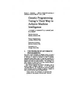
Figure 1 shows the three-dimensional arrangement of the non-hydrogen atoms of BPTI as a stick diagram (i.e., where there is an atom at each intersection or endpoint of the diagram).
Background and introduction
Proteins are responsible for such a wide variety of biological structures and functions that it can be said that the structure and functions of living organisms are primarily determined by proteins (Stryer 1995). Proteins are composed of a chain of amino acid residues in a linear arrangement. The same 20 amino acid residues (denoted by the letters A, C, D, E, F, G, H, I, K, L, M, N, P, Q, R, S, T, V, W, and Y) are used for virtually all proteins of all species on earth. Thus, a protein can be viewed as a linear sequence over a 20-letter alphabet (called the primary structure of the protein). The length of protein sequences vary widely, with the average being
Figure 1 Three-dimensional structure of bovine pancreatic trypsin inhibitor. Amazingly, subject to only a few minor qualifications, it is broadly true that the three-dimensional location of every atom of a protein molecule in a living organism (called its conformation or tertiary structure) is fully determined by this linear sequence over the 20-letter alphabet (Anfinsen 1973). The three-dimensional
arrangement of the atoms, in turn, determines the biological function of a protein within a living organism. That is, all of the information about the biological function of a protein is contained (albeit hidden) in the linear sequence over the 20-letter alphabet. A major goal of the field of computational molecular biology is to determine the biological function of a protein by analyzing the sequence. Ever-growing numbers of primary sequences are being archived in computerized databases (e.g., the SWISSPROT database of Bairoch and Boeckmann 1991) as a consequence of the various ongoing genome projects around the world. As newly sequenced proteins are archived, they are typically immediately tested by various computerized algorithms for clues as to their biological structure and function. One question about a new protein involves its cellular location – that is, where the protein resides in a living organism. After a protein is produced inside the cell, it may perform its work from an intracellular location; it may be expelled from the cell and operate from an extracellular location; it may become embedded in the cell (or other) membrane; or it may reside in the cell's nucleus (if the cell has one).
1.1 Single-residue statistics One very simple type of computation for studying the primary structure of a protein is to compute the protein's amino acid composition (i.e., the percentage of occurrence of each of the 20 amino acids in the protein). Cedano, Aloy, Perez-Pons, and Querol (1997) recently reported in the Journal of Molecular Biology, a single-residue statistical algorithm with 76% accuracy that used the protein's amino acid composition for classifying a protein sequence according to its cellular location using five classes – extracellular (E), intracellular (I), nuclear (N), membrane integral (M), and membrane anchored (A). Their single-residue statistical algorithm works because there are several relatively simple relationships between a protein's cellular location and the frequency of occurrence of particular amino acids. For example, extracellular proteins have a comparatively low percentages of hydrophobic (water-hating) residues and a comparatively high percentage of cysteine residues, which often form extremely stable extracellular disulfide bonds. Integral membrane and anchored membrane proteins are comparatively rich in hydrophobic residues because portion(s) of the protein sequence are embedded in the lipid membrane and hydrophobic residues are congenial to nonpolar environments. Nuclear proteins have comparatively very high percentages of positively charged residues, but comparatively low percentages of aromatic residues. Intracellular proteins have a comparatively high percentages of negatively charged residues and aliphatic residues, but relatively low percentages of cysteine.
1.2 Adjacent-pair-statistics Cedano, Aloy, Perez-Pons, and Querol themselves acknowledged that their single-residue statistical algorithm "is an apparently simple relationship between amino acid composition and protein class (location)" and that it alone cannot pinpoint the cellular location of a protein. For example, it is from known that augmenting single-residue percentages with two-residue percentages can improve the accuracy of classification (Nakashima and Nishikawa 1994).
1.3 Motifs Another type of computation for examining the primary structure of a protein is to scan a protein sequence for an occurrence of a biologically important short subsequence of consecutive amino acid residues (called a motif). Motifs are defined by regular expressions, such as [LIVM]-[LIVM]-D-E-A-D-X-[LIVM]-[LIVM] A protein is said to satisfy this motif if there is a consecutive subsequence anywhere along the entire protein sequence that matches the defining expression in the following way: The first pair of square brackets indicates that the first residue of the consecutive subsequence of length nine is either L, I, V, or M. The second residue is chosen (independently from the first) from the same set of four. The third, fourth, fifth, and sixth residues are mandatory and must be D, E, A, and D, respectively. The X indicates that the seventh residue can be any of the 20 possible amino acid residues. Finally, the eighth and ninth residues of the motif are each chosen (independently) from the same set of four as before, namely L, I, V, or M. The presence of this motif (called ATP_HELICASE_1 in the PROSITE database of motifs of Bairoch and Bucher 1994) almost perfectly determines whether a given protein is a member of a particular family of helicase proteins involved in the unwinding of the double helix of the DNA molecule during the DNA replication. This family of proteins, called the "D-E-A-D box" family, gets its amusing name from the fact that the amino acid residues D (aspartic acid), E (glutamic acid), A (alanine), and D appear, in that order, in this biologically critical subsequence (Linder et. al. 1989). See Koza and Andre 1997 for discovery of a motif for the he "D-E-A-D box" family of proteins using genetic programming.
1.4 Other types of computation Numerous other types of computation, including neural networks, decision trees, inductive logic programming, etc. have been productively applied to particular problems of computational biology. For example, neural networks typically examine a protein sequence using a fixed-sized window and compute the familiar arithmetic weighted
sum of signals (Rost and Sander 1993). Each of these various types of computation can be used to receive the protein's linear sequence over the 20-letter alphabet as its input and emit a classification decision as its output. However, for each of these types of computation, the allowable computation is highly constrained.
1.5 Shortcomings Highly constrained types of computations have many limitations in attempting to capture the exceedingly complex relationship that links a protein's primary sequence to its biological structure and function. Single-residue statistics reduce the entire protein sequence to 20 percentages. Because single-residue statistics look at the protein through a window of a fixed size (one), they cannot take into account relationships between a combination of two or more residues. Adjacent-pair-statistics similarly employ a fixed window size and similarly ignore relationships involving three of more adjacent residues. They even ignore relationships between two or more non-adjacent residues. Similarly, motifs have a fixed window size and are constrained to set-manipulating operations (e.g., matching, disjunction, conjunction) and cannot do any arithmetic or conditional calculations. They are also narrowly focused on a short localized subsequence of consecutive residues. Neural network approaches are limited to using a fixed window size and to performing a particular single type of arithmetic calculation (layers of weighted sums of inputs). In contrast, ordinary computer programs bring a large and varied arsenal of computational capabilities to bear in solving problems. These capabilities include arithmetic functions, conditional functions, logical operations, internal memory, parameterizable subroutines, data structures (named memory, indexed memory, matrices, stacks, lists, rings, queues, relational memory), iteration, recursion, macro definitions, hierarchical compositions of subprograms, multiple inputs, multiple outputs, etc. In addition, motifs, single-residue statistics, adjacentpair-statistics, neural networks, decision trees, inductive logic programming, and other machine learning techniques are not open-ended in the sense that they all require that the human investigator decide, in advance, the detailed nature of the computation that is to be performed. However, for most complex problems, deciding on the nature of the requisite computation is often, in fact, the problem (or at least a major part of it).
1.6 Genetic programming The problem of discovering biologically meaningful patterns in protein sequences can be recast as a search for a classification-performing computer program of unknown size and shape. When the problem is recast in this way, genetic programming becomes a candidate for solving this type of problem.
Genetic programming is an extension of the genetic algorithm (Holland 1975) in which a computer program is automatically created to solve a problem (Koza 1992; Koza and Rice 1992). Genetic programming starts with a primordial ooze of randomly generated computer programs and then applies the Darwinian principle of survival of the fittest and an analog of the naturallyoccurring genetic operation of crossover (sexual recombination) to breed a new (and often improved) population of programs. The size and shape of the evolved programs is open-ended and is part of the solution delivered by genetic programming, not part of the information supplied in advance by the human investigator. The evolved programs may contain arithmetic functions, conditional operations, set-creating operations, automatically defined functions (Koza 1994a; 1994b, 1994c), iteration-performing branches (Koza 1994a, Koza and Andre 1996), named memory (Koza 1992, 1994a), indexed memory (Teller 1994), and most other constructs of ordinary computer programs. The variety of different capabilities of genetic programming is described in Kinnear (1994), Angeline and Kinnear (1996), Koza, Goldberg, Fogel, and Riolo (1996), Koza et al. (1997), and Banzhaf, Nordin, Keller, and Francone (1997).
1.7 Programmatic motifs A computer program resembles a conventional motif (and the other highly constrained types of computation mentioned above) in that it is a deterministic computation that is performed on a protein sequence in order to decide whether the protein has a certain property. We view a computer program as an extension of the conventional concept of motif. We call the program that genetic programming produces for analyzing a protein a programmatic motif.
1.8 Organization of This Paper This paper applies the concept of programmatic motif to the problem of classifying protein sequences as to their cellular location. Section 2 describes the preparatory steps for applying genetic programming to this classification problem. Section 3 presents the results.
2.
Preparatory steps
Before applying genetic programming to a problem, the user must perform six major preparatory steps, namely (1) identifying the primitive functions of the to-be-evolved programs, (2) identifying the terminals, (3) creating the fitness measure, (4) choosing certain control parameters for the run, (5) determining the termination criterion and method of result designation for the run, and (6) determining the architecture of the overall program.
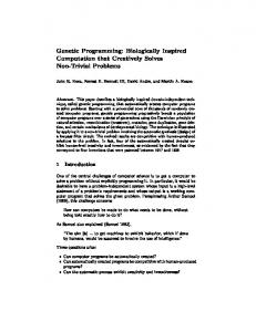
2.1 Architecture As for the architecture of each overall program in the population, we decided that each program would be a multi-part program with seven branches, including three set-creating automatically defined functions (ADF0, ADF1, and ADF2), and two arithmetic-performing automatically defined functions (ADF3 and ADF4), one iteration-performing branch (IPB), and one resultproducing branch (RPB). Figure 2 shows the overall architecture (with just one automatically defined function) of this program.
Here the three-argument conditional branching operator IFGTZ ("If Greater Than Zero") evaluates and returns its second argument if its first argument (the condition) is greater than zero, but otherwise evaluates and returns its third argument. The two-argument protected division function, %, returns the number 1 when division by 0 is attempted (including 0 divided by 0), and, otherwise, returns the normal quotient. The terminal set for the arithmetic-performing automatically defined functions, Tadf-ap, contains the 20 zero-argument numerically-valued residue-detecting functions:
progn looping-overknown-finite-set
defun ADF0
Argument List
values
values
Body of ADF0 Function Definition
Body of Iteration Performing Branch IPB0
Body of ResultProducing Branch RPB
Figure 2 Multi-part program with one automatically defined function, an iterationperforming branch, and a result-producing branch.
2.2 Function and terminal sets The functions and terminals are the ingredients of the tobe-evolved computer program. They are discussed below for the four types of branches used here – the set-creating automatically defined functions, the arithmetic-performing automatically defined functions, the iteration-performing branch, and the result-producing branch. The three set-creating automatically defined functions (ADF0, ADF1, and ADF2) provide a mechanism for defining subsets of the 20 amino acids (that is, for reducing the 20-letter alphabet to a smaller alphabet). The terminal set for the set-creating automatically defined functions, Tadf-sc, contains the 20 zero-argument numerically-valued residue-detecting functions: Tadf-sc = {(A?), (C?), …, (Y?)}. Here (A?) is the zero-argument residue-detecting function returning a numerical +1 if the ACTIVE residue (see below) is alanine (A) but otherwise returning a numerical –1 (and similarly for the 19 other functions (C?), …, (Y?)). The function set for the set-creating automatically defined functions, Fadf, is Fadf-sc = {ORN}. Here ORN is the two-argument numerical-valued disjunctive function returning +1 if either or both of its arguments are positive, but returning –1 otherwise. The two arithmetic-performing automatically defined functions (ADF3 and ADF4) provide a mechanism for performing arithmetic (instead of set-creating) calculations. The function set for the arithmetic-performing automatically defined functions, Fadf-ap, is Fadf-ap = {+, –, *, %, IFGTZ, ORN}.
Tadf-ap = {(A?), (C?), …, (Y?), ←}. Here ← denotes floating-point random constants between –10.000 and +10.000. The iteration-performing branch provides a mechanism for performing an iterative calculation over the entire protein sequence. The proteins are of different length. The work-performing steps of the iteration-performing branch are performed iteratively for each of the amino acid residues of the protein. The iteration over the protein sequence is indexed by the iterative variable INDEX. At the beginning of each step of the iteration, the ACTIVE residue is the same as INDEX. However, the ACTIVE residue can be incremented within a given step of the iteration (the current residue) using the FORWARD function (described below). Memory cells can be used to store the intermediate and final results during the iterative calculation. There are two types of memory – five cells of named memory and 20 cells of indexed memory. The contents of all cells of named and indexed memory are initialized to zero before execution of the iteration-performing branch for a particular fitness case. The calculation in the iteration-performing branch can involve arithmetic functions, conditional operations, the residue-detecting functions, the numerically-valued disjunctive function, the contents of the memory cells, memory-setting functions for the memory cells, and the results produced by the set-creating and arithmeticperforming automatically defined functions. The terminal set for the iteration-performing branch, Tipb, contains the five automatically defined functions (ADF0, ADF1, ADF2, ADF3, ADF4), 20 zero-argument numerically-valued residue-detecting functions, five settable named variables M0, M1, M2, M3, and M4, the READ–RESIDUE function, and floating-point random constants, ←. That is, Tipb = {ADF0, ADF1, ADF2, ADF3, ADF4, (A?), (C?), …, (Y?), M0, M1, M2, M3, M4, READ–RESIDUE, ←bigger-reals}. The terminal M0 returns the value contained in memory cell M0 (and similarly for the four other terminals M1, M2, M3, and M4).
The terminal READ–RESIDUE returns the value contained in the cell of indexed memory implicitly indexed by the active residue. The function set for the iteration-performing branch, Fipb contains numerically valued Boolean disjunction ORN, IFGTZ, FORWARD, the five named setting functions (SETM0, SETM1, ..., SETM4), and the four arithmetic functions. Fipb = {ORN, SETM0, SETM1, SETM2, SETM3, SETM4, IFGTZ, WRITE–RESIDUE, +, -, *, %, FORWARD} The one-argument setting function SETM0 sets settable memory cell M0 to a particular value (and similarly for the four other functions (SETM1, SETM2, SETM3, SETM4). The one-argument WRITE–RESIDUE function sets into the cell of indexed memory implicitly indexed by the active residue to the value of its argument. The one-argument FORWARD function increments the ACTIVE residue by one and returns the value of its one argument using the current value of ACTIVE. Upon completion of the evaluation of the argument of the FORWARD function, the ACTIVE residue is restored to its previous value. If the FORWARD function attempts to increment the ACTIVE residue beyond the length of the protein, the ACTIVE residue remains as the last residue of the protein. Note that the values (+1 or –1) returned by the five automatically defined functions depend on the ACTIVE residue. The result-producing branch provides a mechanism for performing a final calculation that classifies the protein into one of two classes. The terminal set for the result-producing branch, Trpb, is Trpb = {M0, M1, M2, M3, M4, ←}. The function set for the result-producing branch, Frpb, is Frpb = {ORN, IFGTZ, +, -, *, %, READ} The one-argument READ function returns the value stored in the indexed memory cell J where J is the value of its one argument modulo 20. The wrapper (output) interface for the result-producing branch consists of the IFGTZ function, so a positive return value is interpreted as YES and a zero or negative return value is interpreted as NO.
2.3 Fitness The fitness measure indicates how well a particular genetically-evolved program classifies protein sequences. Fitness is measured over a number of protein sequences (fitness cases). When a classifying program is tested against a particular protein sequence, the outcome can be a true-positive, true-negative, false-positive, or falsenegative. The total number of true-positives, true-
negatives, false-positives, and false-negatives for a set of protein sequences, in turn, can be used to compute the correlation coefficient, C, where
C=
(N
tn
Ntp Ntn − N fn N fp
+ N fn )(Ntn + N fp )(Ntp + N fn )(Ntp + N fp )
The fitness of a classifying program is then be defined as 1−C . Thus, fitness ranges between 0.0 and +1.0, so that 2 lower values of fitness are better than higher values and a value of 0 corresponds to the best. Cedano, Aloy, Perez-Pons, and Querol 1997 used 1,000 proteins (200 from each of five classes) as their insample fitness cases. We reduced computer time by about three-fourths by randomly choosing 50% of Cedano's proteins that were of length less than 600 (i.e., about twice the length of an average-sized protein) as our in-sample fitness cases. This approach yielded 471 in-sample fitness cases (88 membrane, 91 nuclear, 108 intracellular, 124 extracellular, and 70 anchored proteins) having a total of 122,489 residues. The true measure of performance for a predicting program is how well it generalizes to unseen additional (out-of-sample) fitness cases. The results were first cross-validated using the remaining proteins of length less than 600. Then, the results were further crossvalidated using the same 200 out-of-sample fitness cases as in Cedano, Aloy, Perez-Pons, and Querol 1997 (specifically, 41 membrane, 46 nuclear, 55 intracellular, 33 extracellular, and 25 anchored proteins) having a total of 100,029 residues). Considerable computer time was saved by caching the result of executing each set-creating and arithmeticperforming automatically defined function for each of the 20 residues. The population size was 320,000. The control parameters for the run were the same as those in Koza 1994a, except (1) the maximum size, Hrpb, for the resultproducing branch is 400 points, (2) the maximum size, Hadf, for each automatically defined function is 40 points, and (3) the maximum size, Hipb, for the iterationperforming branch is 400 points. The problem was run on a medium-grained parallel Parsytec computer system consisting of 64 80-MHz Power PC 601 processors arranged in a toroidal mesh with a host PC Pentium type computer. The distributed genetic algorithm was used with a population size of Q = 5,000 at each of the D = 4 demes. On each generation, four boatloads of emigrants, each consisting of B = 2% (the migration rate) of the node's subpopulation (selected on the basis of fitness) were dispatched to each of the four toroidally adjacent nodes (Andre and Koza 1996).
3.
Results
On generation 26, genetic programming evolved a twoway classification program for extracellular proteins with
82% in-sample accuracy, 87% out-of-sample accuracy (on-line), and 83% accuracy on the 200 out-of-sample proteins (off-line) of Cedano et al. 1997. This result was obtained on the one and only run of genetic programming for the problem of classifying proteins that we made. The genetically evolved program referred once to its arithmetic-performing automatically defined function ADF4 and repeatedly referred to its set-creating automatically defined function ADF1. It twice used the FORWARD function to examine downstream residues. It used one cell of named memory (M0) for communication between its iteration-performing branch and the resultproducing branch.
4.
Conclusion
A two-way classification program for identifying extracellular proteins using programming motifs and genetic programming produced a two-way classifier with 83% accuracy on the 200 out-of-sample proteins (off-line) of Cedano et al. 1997. This result is competitive with the 76% accuracy of the human-created five-way algorithm for cellular location created using statistical techniques (Cedano et al. 1997).
References Andre, David and Koza, John R. 1996. Parallel genetic programming: A scalable implementation using the transputer architecture. In Angeline, P. J. and Kinnear, K. E. Jr. (editors). 1996. Advances in Genetic Programming 2. Cambridge: MIT Press. Anfinsen, C. B. 1973. Principles that govern the folding of protein chains. Science 81: 223-230. Angeline, Peter J. and Kinnear, Kenneth E. Jr. (editors). 1996. Advances in Genetic Programming 2. Cambridge, MA: The MIT Press. Bairoch, A. and Boeckmann, B. 1991. The SWISS-PROT protein sequence data bank: current status. Nucleic Acids Research 22(17) 3578–3580. Bairoch, Amos and Bucher, Philipp. 1994. PROSITE: Recent developments. Nucleic Acids Research 22(17) 3583-3589. Banzhaf, Wolfgang, Nordin, Peter, Keller, Robert E., and Francone, Frank D. 1997. Genetic Programming – An Introduction. San Francisco, CA: Morgan Kaufmann and Heidelberg: dpunkt. Cedano, Juan, Aloy, Patrick, Perez-Pons, Josep A., and Querol, Enrique. 1997. Relation between amino acid composition and cellular location of proteins. Journal of Molecular Biology. 266(3) 594 – 600. Holland, John H. 1975. Adaptation in Natural and Artificial Systems. Ann Arbor, MI: University of Michigan Press. Kinnear, Kenneth E. Jr. (editor). 1994. Advances in Genetic Programming. Cambridge, MA: MIT Press. Koza, John R. 1992. Genetic Programming: On the Programming of Computers by Means of Natural Selection. Cambridge, MA: MIT Press. Koza, John R. 1994a. Genetic Programming II: Automatic Discovery of Reusable Programs. Cambridge, MA: MIT Press.
Koza, John R. 1994b. Genetic Programming II Videotape: The Next Generation. Cambridge, MA: MIT Press. Koza, John R. 1994c. Architecture-Altering Operations for Evolving the Architecture of a Multi-Part Program in Genetic Programming. Stanford University Computer Science Department technical report STAN-CS-TR-94-1528. October 21, 1994. Koza, John R. and Andre, David. 1996. Evolution of iteration in genetic programming. In Fogel, Lawrence J., Angeline, Peter J. and Baeck, T. 1996. Evolutionary Programming V: Proceedings of the Fifth Annual Conference on Evolutionary Programming. Cambridge, MA: The MIT Press. Pages 469 – 478. Koza, John R. and Andre, David. 1997. Automatic discovery of protein motifs using genetic programming. In Yao, Xin (editor). 1997. Evolutionary Computation: Theory and Applications. Singapore: World Scientific. In Press. Koza, John R., Deb, Kalyanmoy, Dorigo, Marco, Fogel, David B., Garzon, Max, Iba, Hitoshi, and Riolo, Rick L. (editors). 1997. Genetic Programming 1997: Proceedings of the Second Annual Conference, July 13–16, 1997, Stanford University. San Francisco, CA: Morgan Kaufmann. Koza, John R., Goldberg, David E., Fogel, David B., and Riolo, Rick L. (editors). 1996. Genetic Programming 1996: Proceedings of the First Annual Conference, July 28-31, 1996, Stanford University. Cambridge, MA: MIT Press. Koza, John R., and Rice, James P. 1992. Genetic Programming: The Movie. Cambridge, MA: MIT Press. Kyte, J. and Doolittle, R. 1982. A simple method for displaying the hydropathic character of proteins. Journal of Molecular Biology. 157:105-132. Linder, P., Lasko, P., Ashburner, M., Leroy, P., Nielsen, P. J., Nishi, J., Schneir, J., and Slonimski, P. P. 1989. Birth of the D–E–A-D box. Nature 337: 121–122. Nakashima, J. and Nishikawa, K. 1994. Discrimination of intercellular and extracellular proteins using amino acid composition and residue-pair frequencies. Journal of Molecular Biology. 238: 54 – 61. Rost, B. and Sander, C. 1993. Prediction of protein secondary structure at better than 70% accuracy. Journal of Molecular Biology. 232: 584 – 599. Stryer, Lubert. 1995. Biochemistry. New York, NY: W. H. Freeman. Fourth Edition. Teller, A. (1994). The evolution of mental models. In Kinnear, K. E. Jr. (editor). Advances in Genetic Programming. Cambridge, MA: The MIT Press. Pages 199 – 219.
Version 2 – Paper 2039 - Camera-Ready – Submitted January 7, 1998 to the 1998 IEEE International Conference on Evolutionary Computation (ICEC-98) to be held in Anchorage, Alaska on May 5-9, 1998.
Classifying Proteins as Extracellular using Programmatic Motifs and Genetic Programming John R. Koza
Forrest H Bennett III
David Andre
Computer Science Dept. Stanford University Stanford, California 94305-9020
[email protected] http://www-csfaculty.stanford.edu/~koza/
Visiting Scholar Computer Science Dept. Stanford University Stanford, California 94305
[email protected]
Computer Science Division University of California Berkeley, California 94720
[email protected]
KEYWORDS: Genetic programming, molecular biology, classification