data abstraction levels. The features are represented by attribute sets, which play a key role in the visualization process. Icons are symbolic parametric objects, ...
Iconic Techniques for Feature Visualization Frank J. Post Theo van Walsum Frits H. Post Delft University of Technology � Deborah Silver Rutgers University Abstract This paper presents a conceptual framework and a process model for feature extraction and iconic visualization. Feature extraction is viewed as a process of data abstraction, which can proceed in multiple stages and corresponding data abstraction levels. The features are represented by attribute sets, which play a key role in the visualization process. Icons are symbolic parametric objects, designed as visual representations of features. The attributes are mapped to the parameters (or degrees of freedom) of an icon. We describe some generic techniques to generate attribute sets, such as volume integrals and medial axis transforms. A simple but powerful modeling language was developed to create icons, and to link the attributes to the icon parameters. We present illustrative examples of iconic visualization created with the techniques described, showing the effectiveness of this approach. Keywords: scientific visualization, feature extraction, iconic visualization, attribute set.
1 Introduction Visualization techniques provide tools for obtaining information from data, ranging from simple presentation techniques, that just display the data, to sophisticated techniques that extract and display the information automatically. In this paper, we present a visualization approach to create abstract visualizations of data sets. This approach entails the extraction of features and the use of icons for data visualization. An icon as we use it, is a geometric object with parametric geometry and visual attributes that can be arbitrarily � Faculty of Technical Mathematics and Informatics, Julianalaan 132, 2628 BL Delft, The Netherlands �� Dept. of Electrical and Computer Engineering, Laboratory for Visiometrics and Modeling, P.O. Box 1390, Piscataway, NJ 08855-1390, USA
��
linked to data quantities. The function of an icon is to act as a symbolic representation, which shows essential characteristics or features of a data domain to which the icon refers. Reduction to essentials is the main purpose of the use of icons: to replace the original data by a symbolic representation that is more clear, compact, and meaningful, and which is related to the physical concepts of an application [15]. Icons have been studied extensively in many fields, such as in logic, the theory of signs or semiotics [9], and in pictorial information systems [5]. An attempt to relate the meaning of icons for visualization to classical sign theory has recently been made by Hesselink and Delmarcelle [13]. In scientific visualization, the icon concept is related to the Abstract Visualization Objects [12], and Parametric Graphic Objects used for computational steering [24]. The term ‘glyph’ has also been frequently used [16], which is roughly comparable to the term icon as it is used here. Early applications of iconic visualization can be found in statistical data visualization, such as Kleiner-Hartigan trees [4] and Chernoff faces [6]. These techniques are used for high-dimensional data that are defined in an abstract data space, and not in Euclidean physical space. Examples of iconic representations in scientific visualization are glyphs used by Globus et al. [11] to indicate location and type of critical points in a vector field, and cylindrical objects to visualize vortex tubes extracted from flow fields [2, 22]. Ellipsoids have also been used as icons for feature visualization [17, 19, 25]. Our purpose in this paper is to demonstrate the generation and use of macroscopic icons for visualization of features and feature attributes. Features can be represented by attribute sets. Icons provide a natural way for their visualization, by linking the attributes to their parameters. We discuss iconic representations in Section 2. Then we discuss how a visualization process model can be adapted for feature extraction and iconic visualization, and how feature extraction can be represented as a multi-level process of data abstraction (Section 3). Then we show in Sec-
tion 4 some examples of feature attribute calculation. In Section 5, a simple icon specification and attribute mapping technique is described, and in Section 6 the use of these techniques is demonstrated with some applications of iconic feature visualization. In Section 7, we present conclusions and directions for further research.
2 Iconic representation The general meaning of the term ‘icon’ is a conventional pictorial representation, or a sign sharing a property with the thing it represents. We will not formally define the concept here, but use a simple definition that suits our purpose, and briefly review the role that icons can play in scientific visualization and especially in feature visualization. A first important aspect is the number of degrees of freedom, or parameters, that can be varied for the icon, and separately bound to data quantities. The parameters can be divided into three groups: spatial parameters (position and orientation), geometric parameters which control the shape of the object, and descriptive parameters such as color, texture, transparency, or sound. If the number of parameters is indefinite, this means that the icon is a (quasi-)continuous geometric object: a curve, surface, or solid. For example, a streamline represents a large, indeterminate number of sample points in a velocity field. By contrast, an arrow icon in a 3D vector field has only six spatial and geometric parameters: position, direction, and length. Examples of geometric objects are iso-surfaces, streamlines, stream surfaces, tensor field lines or hyper-streamlines [13], skeletons [20], and vortex tubes [2, 22]. The reference domain is the spatio-temporal area for which the attribute set has been calculated, and that is represented by a single icon. Local means a point and its infinitesimal environment, as represented by gradients. Intermediate is the level of a sub-volume, at a scale between local and global, which can apply to features or selections [23]. An icon that can be used at different levels is the ellipsoid. This object can be used for visualization of the eigenvalues and eigenvector directions of second order tensors [10]. It has been applied to visualize stress tensors [12], but it can also be used for fitting an object to an irregular-shaped area. The spatial distribution of an area is characterized by the tensor of second moments, which is visualized by an ellipsoid. The icon then shows a simplified representation of the shape of the area [19]. The display domain is the space in which the iconic objects exist, which is not the display screen, but the graphical object space. Time-dependent attribute bindings are considered as a separate dimension, shown by animation
of changing shape or other attributes reflecting parameter variations. The display scale refers to relative size. Micro-icons are discrete, but not quite individual objects; they can only exist in large quantities, as elements of dot or line patterns or texture elements; meaning emerges from them only in large numbers. Examples at this level are markers, arrows, stick figures [8, 21], and particles. At the intermediate scale level, the icons are more distinct but they are still used in large numbers. Examples are simple 3D solids [16], wedges [7], or polygons. At the largest scale, icons are individual objects representing data attributes from a given reference domain. Examples of this type are Chernoff faces [6], ellipsoids [19], and the flow probe [14]. A last aspect is the use of icons for interaction. A passive icon is used for display purposes only. Position and appearance are dictated by the data. An icon that can be interactively positioned at a chosen reference point can be used as a probe [14]. If the data binding is in two directions, icons may be used to control model parameters in interactive steering of simulations [24].
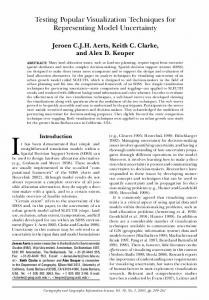
3 A process model for multilevel iconic feature visualization For the iconic visualization process, a process model, based on the visualization pipeline [12], can be used (see Figure 1). The goal of the iconic representation is to get a ‘summarized’ visualization, therefore the first step in the iconic visualization process is to find items in the dataset that need to be represented in the summary, i.e. data that are important or relevant in some respect (features). Simultaneously, or in the next processing step, characteristic parameter values of the features (attributes) are calculated. This is what we call feature extraction and attribute calculation. The result of this feature extraction is a set of attribute values that characterize the feature. This is called an attribute set; each characteristic value is an attribute of the feature. As the attribute set represents the data at another, higher level, this is a process of data-abstraction. The feature extraction and attribute calculation stage can be implemented in different ways. Special algorithms can be developed to extract specific features from data and calculate the attribute sets [2, 22]. An alternative approach is to use general selection and segmentation techniques to identify features in the data [19, 20, 23]. Attributes can be calculated with volume integrals over the selected region, or image processing techniques such as skeleton extraction. In the iconic mapping stage, the attributes are mapped onto the parameters of icons. The purpose of this mapping is to visualize features by objects, that display the char-
data reduction
data generation
field data
attribute sets
visualization
feature extraction attribute calculation
abstraction
abstraction
......
original
attribute
attribute
data
set 1
set 2
primary
secondary
direct
indirect
indirect
mapping
mapping
mapping
iconic mapping visual primitives
display
Figure 1: Iconic visualization pipeline. acteristics of a feature in a clear and understandable way: there should be some similarity relation between the features and their iconic representations. The way the attributes are mapped onto the icon’s parameters determines the appearance of the icon. One important consequence of this process is a vast data reduction. The original data field is replaced by a usually small number of attribute sets, visualized by simple geometric objects. The reduction is caused by the data selection and abstraction, and is necessary for understanding the information inherent in very large data sets. The size of a typical CFD data set will be in the order of 10-100 Mbytes per time step. For 100 features of 20 data items, the feature/attribute dataset will be in the order of 10 Kbytes. This attribute set represents one specific view of the data set, which may for its purpose replace the original data set, and thus means a reduction by a factor of at least 1000. An icon will be in the order of 100s of polygons, so the total visualization may be about 104 to 105 polygons, which can be displayed by a graphics workstation in real time. The size of the intermediate attribute data set is very small, and this provides an excellent opportunity for distributed processing. The computationally and data intensive first part of the process can be executed on a remote highperformance computer, and the results can be easily transferred to the visualization workstation by a low-bandwidth link. The abstraction process can be applied recursively, resulting in a series of attribute sets, each representing the data at a different level of abstraction. The data at each level of abstraction can be visualized with a symbolic representation: an icon. The level of abstraction of the symbolic representation increases if the level of abstraction of the data increases: a more abstract data representation gives a more abstract visual representation. Also, the semantics of
standard visualization
iconic visualization
Figure 2: Multilevel feature extraction. an attribute set can be enriched in the process of abstraction. This is depicted in Figure 2. The upper line shows the multilevel abstraction process, of which data reduction is an important side-effect. At each abstraction level, the attribute sets can be mapped onto symbolic representations (icons), yielding an iconic visualization of the data. Visualization mapping without a distinct abstraction is called direct mapping (e.g. arrow plot, isosurface). Mappings with one or more levels of abstraction are called indirect mappings. The lower pictures show examples of visualizations that correspond to the data abstraction process.
4 Attributes The set of characteristic values (the attribute set) can consist of a combination of scalars, vectors, and tensors. Attributes can be classified by type of information they carry. Geometric/morphological attributes, such as width, height, volume, centroid, and shape, describe the spatial properties, of a feature. Data attributes, such as minima and maxima, describe the properties of the data over a feature. Combined morphological/data attributes, such as center of gravity in a density field, describe both spatial and data properties of a feature.
4.1 Attribute calculation Of course, the number of techniques to generate attribute sets is unlimited. In this description of attribute calculation we restrict ourselves to three generic techniques, integration, medial axis transform and interpolation. A feature in a dataset may be larger than a single grid position or cell. We can use a selection technique [23] or
a special algorithm to extract a region from the dataset that ‘contains’ the feature. In that case, relevant attributes such as volume, center, mean velocity and moments can be calculated using volume integrals. These volume integrals are calculated with standard quadrature techniques. We have developed software with which we can calculate integrals of arbiratry functions over a selected volume. Skeletal representations of objects are fundamental to the field of mathematical morphology [18]. These representations depict the object as a line segment in two or three dimensions (a low-order approximation) equivalent to using a stick figure to represent a person. They are useful for feature time tracking [22], depicting movement and overall shape change. Furthermore, these approximations can help in reduced model formation. Therefore, medial axis transform is a relevant method to generate attribute sets for selected regions in the data. The attribute sets then contain data on the medial axis. Because the field is continuous, both geometric (utilizing boundary information) and numeric methods can be used to generate a skeleton. Geometric techniques generally are thinning operations [18], while numeric methods use tracing techniques [2, 22]. Path lines and vector directions can be used to guide the ‘medial axis’ search. Interpolation can also be considered as a method to extract attributes. For a given point in the dataset, the data value is interpolated. Differential properties at that location can be calculated as well, for example the velocity gradient tensor in a velocity field. The resulting attribute set represents local data values, and can be used if the feature to be visualized is restricted to a position in a dataset, such as a critical point.
4.2 Further abstraction of attribute sets In the previous sections techniques have been described to extract attribute sets from datasets. It is possible, however, to make further abstractions of attribute sets in order to reduce the size or enrich the semantics of the attribute sets. We illustrate this with an ellipse fitting technique. The ellipse or ellipsoid is a shape generic to almost all simulations. Furthermore, elliptical boundaries are an exact solution for a class of 2D incompressible flows, and they can be easily tracked over time. These regions can be well approximated by physical-space moments (which can be used to classify shapes, as well as visualize them). For example, by isolating regions of the field and then computing the second moments, essential information at a first level of quantification is obtained. The second moments define a tensor, which can be associated with an oriented ellipsoid. Even when the topology of the features is inadequately represented by ellipsoids, the fitted ellipsoid still provides a sense of position, orientation, and relative weight
to the region [19]. Higher-order moments can determine the ‘goodness’ of the fit for classification and are also useful in pattern recognition. In addition, they can define additional parameters with which to ‘deform’ the ellipse to a better fitting icon. If the centroid and a covariance matrix have been generated as a representation of the shape of an area, an ellipsoid can be directly constructed from these values, but the construction may be easier if the eigenvalues and eigenvectors of the covariance matrix are given. From eigenvectors, eigenvalues and the position, an ellipsoid can be constructed in space. These values are easier to interpret than a covariance matrix. Abstractions like these can be performed in a number of ways. These operations can be simple linear functions, but can also be an iterative diagonalization process such as the ‘Cyclic Jacobi’ algorithm, or tensor transformations.
5 Modeling of icons In the previous section, we stated that the number of different types of features is unlimited. The number of different types of icons is likewise unlimited. Therefore, for iconic visualization, one needs either a large set of icons, sufficient for the visualization of features for a specific application area, or an icon design system, with which researchers can develop their own iconic representation of features. The development of a sophisticated interactive icon design system is beyond the scope of our work. Also, we did not generate a large set of icons for a specific application area. However, in order to facilitate the construction of icons, we developed a simple but powerful icon modeling language, with which we were able to generate a set of very different icons. With this language, geometrical primitives can be defined and the parameters of these primitives can be bound to the attribute set. The geometric primitives are constructed with this language in three steps: 1. A 2D contour in the x-y plane is designed and colors or color-maps are bound to this contour. This contour can consist of line-segments or parametric functions. The coordinates of the line-segments, the constants of the parametric functions and the colors or color-maps can be bound to the attribute set. 2. This contour is extended to a 3D object by performing a rotation sweep around the x or y axis, performing a translation sweep by moving the contour along an axis over a given length,or performing a general sweep along a arbitrary 3D trajectory [3]. The parameters of the function that defines the 3D trajectory can also be bound to the attribute set.
Bind_Trans(T012,a[0],a[1],a[2]) /* binding of T012 */ Bind_Rot(AnglesFromVec_3_4_5, /* binding of Angles... */ 0, -asin(a[5]/sqrt(a[3]*a[3]+a[4]*a[4]+a[5]*a[5])), a[3]>0 ? atan (a[4]/a[3]) : a[3]