J. Korean Math. Soc. 47 (2010), No. 5, pp. 1077–1095 DOI 10.4134/JKMS.2010.47.5.1077
IDENTIFIABILITY FOR COMPOSITE STRING VIBRATION PROBLEM Semion Gutman and Junhong Ha Abstract. The paper considers the identifiability (i.e., the unique identification) of a composite string in the class of piecewise constant parameters. The 1-D string vibration is measured at finitely many observation points. The observations are processed to obtain the first eigenvalue and a constant multiple of the first eigenfunction at the observation points. It is shown that the identification by the Marching Algorithm is continuous with respect to the mean convergence in the admissible set. The result is based on the continuous dependence of eigenvalues, eigenfunctions, and the solutions on the parameters. A numerical algorithm for the identification in the presence of noise is proposed and implemented.
1. Introduction Consider the transverse vibration of a thin string of length 1 stretched with a unit force. Let the string be made of finitely many uniform pieces. Let its density be ρ(x), and the piecewise constant parameter a(x) = 1/ρ(x) satisfy 0 < ν ≤ a(x) ≤ µ, x ∈ [0, 1] with a(x) = ai for x ∈ [xi−1 , xi ), i = 1, 2, . . . , N . Then the string’s displacement from the position of equilibrium u(x, t), 0 ≤ x ≤ 1, t > 0 can be modeled by utt − (a(x)ux )x = f (x, t), x 6= xi , t ∈ (0, T ), u(0, t) = q1 (t), u(1, t) = q2 (t), t ∈ (0, T ), u(xi +, t) = u(xi −, t), (1.1) a(xi +)ux (xi +, t) = a(xi −)ux (xi −, t), u(x, 0) = g(x), ut (x, 0) = h(x), x ∈ (0, 1). The parameter identification problem for (1.1) is to find variable parameters a, f, q1 , q2 and g such that the solution u(x, t) fits given observations z in a prescribed (e.g., the best fit to data) sense. The identifiability problem for (1.1) is to establish the uniqueness of the above identification. Received January 30, 2009; Revised June 4, 2009. 2000 Mathematics Subject Classification. 35R30, 93B30. Key words and phrases. identification, identifiability, piecewise constant parameters, string vibration. c °2010 The Korean Mathematical Society
1077
1078
SEMION GUTMAN AND JUNHONG HA
One can view such a model as a special case of the remote sensing problem. When identifiability results are available, the system can be designed accordingly. Our main results are contained in Section 3. There we consider the string vibration problem
(1.2)
utt − (a(x)ux )x = 0, x 6= xi , t ∈ (0, T ), u(0, t) = 0, u(1, t) = 0, t ∈ (0, T ), u(xi +, t) = u(xi −, t), a(x i +)ux (xi +, t) = a(xi −)ux (xi −, t), u(x, 0) = g ∈ H01 [0, 1], ut (x, 0) = h ∈ L2 [0, 1]
and show that the piecewise constant parameter a(x) can be uniquely identified from finitely many observation functions zm (t) = u(pm , t), t > 0, m = 1, 2, . . . , M − 1. These observations should be taken at a sufficiently dense in (0, 1) set of equidistant points pm as specified in Theorem 3.3. Also in this section we show that the identification is stable, i.e., the recovered parameters a depend continuously on the observations zm (t). These results use certain properties of solutions of (1.2) established in Section 2. The main idea of our identification method is to use the Fourier transform of the data zm (t) to find the first eigenvalue λ1 of the associated Sturm-Liouville problem and a constant multiple Cψ1 (pm ) of the first eigenfunction at the observation points. The resulting sequence of M numbers (denoted by G) provides the input to the Marching Algorithm (see [7]) which uniquely recovers the sought parameter a(x). In Section 4 the identifiability results are generalized to problems with nonzero boundary inputs q1 (t) and q2 (t), as well as for a nonzero external input f (x, t). In Section 5 we present numerical results illustrating the identification of a piecewise constant parameter a(x) from the observations zm (t) of the system. Some identifiability results for smooth or constant parameters a were obtained previously, see [14, 15, 16]. These works show that one can identify a constant parameter a in (1.2) from the measurement z(t) taken at one point p ∈ (0, 1). These works also discuss problems more general than (1.2), including problems with a broad range of boundary conditions, non-zero forcing functions, as well as elliptic and parabolic problems. In [12], [4] and references therein identifiability results are obtained for elliptic and parabolic equations with discontinuous parameters in a multidimensional setting. A typical assumption there is that one knows the normal derivative of the solution at the boundary of the region for every Dirichlet boundary input. Different approaches can be found in [1, 3] and in more comprehensive treatments [2, 10, 11]. In [7] and [8] we studied the conductivity identifiability problems and obtained some fundamental results (the Marching Algorithm, the continuity of the
COMPOSITE STRING VIBRATION
1079
eigenvalues and the eigenfunctions) critical for the string vibration problems studied in this paper. 2. Properties of solutions Let the admissible set be defined by Aad = {a ∈ L∞ [0, 1] : 0 < ν ≤ a(x) ≤ µ} for some positive constants ν and µ. Admissible sets of piecewise constant parameters are defined as follows. Definition 2.1. (1) Define PC = ∪∞ N =1 PC N ⊂ Aad , where PC N consists of piecewise constant functions a(x) of the form a(x) = ai for x ∈ [xi−1 , xi ), i = 1, 2, . . . , N . (2) Let σ > 0. Define PC(σ) = {a ∈ PC : xi − xi−1 ≥ σ,
i = 1, 2, . . . , N },
where x1 , x2 , . . . , xN −1 are the discontinuity points of a, and x0 = 0, xN = 1. Note that a ∈ PC(σ) attains at most N = [[1/σ]] distinct values ai , 0 < ν ≤ ai ≤ µ. Theorem 2.2. Let a ∈ PC. Then (1) The associated (2.1)
Sturm-Liouville problem for (1.1) (a(x)ψ(x)0 )0 = −λψ(x), x 6= xi , ψ(0) = ψ(1) = 0, ψ(xi +) = ψ(xi −), a(xi +)ψx (xi +) = a(xi −)ψx (xi −)
has infinitely many eigenvalues 0 < λ1 < λ2 < · · · → ∞. 2 The normalized eigenfunctions {ψk }∞ k=1 form a basis in L [0, 1]. (2) Each eigenvalue is simple. For each eigenvalue λk there exists a unique continuous, piecewise smooth normalized eigenfunction ψk (x) such that ψk0 (0+) > 0, and the function a(x)ψk0 (x) is continuous on [0, 1]. Also ψ1 (x) > 0 for x ∈ (0, 1). (3) Eigenvalues {λk }∞ k=1 satisfy the inequality
νπ 2 k 2 ≤ λk ≤ µπ 2 k 2 . These and other properties of the eigenvalues and the eigenfunctions of (2.1) follow from standard arguments, see e.g. [5]. A more detailed derivation is presented in [7] and [8].
1080
SEMION GUTMAN AND JUNHONG HA
Let H = L2 [0, 1] with the norm k · k and the inner product h·, ·i. Let V = H01 [0, 1]. Then (1.2) can be restated as an abstract differential equation within the standard triple V ⊂ H ⊂ V 0 u00 + Au = 0,
(2.2)
u(0) = g ∈ V,
u0 (0) = h ∈ H.
According to [13, 5], equation (2.2) has a unique weak solution u ∈ C([0, T ]; V ). We need a somewhat more detailed information about it. Theorem 2.3. Let a ∈ PC, h ∈ H, g ∈ V . Then on D = [0, 1] × [0, ∞) the weak solution u of (2.2) is given by (2.3)
u(x, t) =
∞ X
p p (Ak cos( λk t) + Bk sin( λk t))ψk (x)
k=1
with (2.4)
Ak = hg, ψk i,
hh, ψk i Bk = √ , λk
k = 1, 2, . . . .
Moreover, the series in (2.3) converges uniformly on D, and the solution u(x, t) is a continuous and bounded function in D. Proof. The partial sums in (2.3) are Galerkin approximations for the solution of (2.2). Their weak convergence to the solution u(x, t) is established using the energy estimate as in [13] or [5]. Under our assumptions it takes the form of the energy conservation Z 1 Z 1 2 2 (2.5) (a(x)|ux (x, t)| + |ut (x, t)| )dx = (a(x)|g 0 (x)|2 + |h(x)|2 )dx 0
0
for each t ≥ 0. We are going to give an explicit derivation of this equality as well as to show the uniform convergence of the involved series. Recall that the eigenfunctions {ψk (x)}∞ k=1 form an orthonormal basis in H. Let the coefficients Ak and Bk be defined as in (2.4). Then ∞ X
|Ak |2 = kgk2H ,
k=1
√
∞ X
λk |Bk |2 = khk2H .
k=1
λk }∞ k=1
Also functions {ψk / form an orthonormal basis in Va , i.e., in V equipped with the equivalent inner product hav 0 , w0 i for v, w ∈ V , see Theorem 6.5.2 in [5]. Thus Z 1 ∞ X λk |Ak |2 = kgk2Va = a(x)|g 0 (x)|2 dx. 0
k=1
Fix t > 0. Then Z kuN (x, t)k2Va =
1 0
¯2 ¯ N ¯ ¯X p p ¯ ¯ a(x) ¯ (Ak cos( λk t) + Bk sin( λk t))ψk0 (x)¯ dx ¯ ¯ k=1
COMPOSITE STRING VIBRATION
=
N X
λk |Ak cos(
1081
p
p λk t) + Bk sin( λk t)|2 ,
k=1
Z 2 |uN t (x, t)kH
1
= 0
=
¯N ¯2 ¯X p ¯ p p ¯ ¯ λk (−Ak sin( λk t) + Bk cos( λk t))ψk (x)¯ dx ¯ ¯ ¯ k=1
N X
p p λk | − Ak sin( λk t) + Bk cos( λk t)|2 .
k=1
Thus Z (2.6) 0
1
2 N 2 (a(x)|uN x (x, t)| + |ut (x, t)| )dx =
N X
λk (A2k + Bk2 )
k=1
and the series in (2.3) converges in Va uniformly with respect to t > 0. Since νkvk2V ≤ kvk2Va and C[0, 1] is continuously imbedded in V it follows that the series in (2.3) converges uniformly on D, and the limit u(x, t) is continuous. Also the norm ku(x, t)kV is uniformly bounded for t > 0, thus u(x, t) is bounded on D. Finally, one obtains (2.5) by taking the limit as N → ∞ in (2.6). ¤ 3. Identification map and its continuity This section contains our main results. Here is an outline of our arguments. Let a ∈ PC and p ∈ (0, 1). Then the string motion at the point p is given by (3.1) ∞ X p p zp (t; a) = u(p, t; a) = (Ak cos( λk t) + Bk sin( λk t))ψk (p; a), t ≥ 0 k=1
with the coefficients Ak and Bk defined in (2.4). By Theorem 2.3, zp (t; a) is a bounded continuous function for t ≥ 0. Our goal is to extract the first eigenvalue λ1 (a) and a constant multiple of the first eigenfunction C(a)ψ1 (p; a) from zp (t; a), with C(a) being independent of the point p ∈ (0, 1). This is accomplished in Theorem 3.1 by applying the Fourier transform to the even or odd extension of zp (t; a). Given M − 1 observation points pm this procedure defines the solution map G(a) by (3.2)
G(a) = (λ1 (a), G1 (a), . . . , GM −1 (a)) ∈ RM ,
a ∈ PC,
where Gm (a) = C(a)ψ1 (pm ; a). Note that the M -tuple G(a) is determined from the observations zm (t; a) = u(pm , t; a) without the knowledge of the parameter a. Suppose that one observes the system (1.2) at sufficiently many observation points pm , m = 1, 2, . . . , M − 1 equidistant on the interval (0, 1) as specified in Theorem 3.3. This theorem asserts that the solution map G(a) can be inverted on PC(σ), i.e., the piecewise constant parameter a can be uniquely identified from G(a).
1082
SEMION GUTMAN AND JUNHONG HA
This inversion procedure is accomplished by the Marching Algorithm described and justified in [7]. The Marching Algorithm ([7], Theorem 4.6) is applied there to the identifiability of piecewise constant conductivities in a heat conduction problem. Since the solution of the heat conduction problem is different from (3.1), a different procedure is used there to extract the M -tuple G(a) from the data. However, the application of the Marching Algorithm to G(a) is the same. Finally in this section, we show that G is continuous (as a function of a) if PC(σ) is equipped with the L1 [0, 1] topology. Observing that PC(σ) is compact in this topology we can conclude that the identification map G −1 is continuous. This means that the identification procedure is stable. Theorem 3.1. Let a, b ∈ PC, g ∈ V, h ∈ H. Let p ∈ (0, 1) and zp (t; a) be defined by zp (t; a) = u(p, t; a), t ≥ 0, where u(x, t; a) is the weak solution of (1.2). (1) Suppose that h = 0. Then the Fourier transform of the even extension zp,even (t; a) of zp (t; a) is given by (3.3)
F(zp,even (t; a)) Z ∞ 1 √ = zp,even (t; a)e−iwt dt 2π −∞ ∞ r h X p p i π = Ak δ(w − λk ) + Ak δ(w + λk ) ψk (p; a). 2 k=1
(2) Suppose that g = 0. Then the Fourier transform of the odd extension zp,odd (t; a) of zp (t; a) is given by (3.4)
F(zp,odd (t; a)) Z ∞ 1 = √ zp,odd (t; a)e−iwt dt 2π −∞ ∞ r h X p i p π = −iBk δ(w − λk ) + iBk δ(w + λk ) ψk (p; a). 2 k=1
(3) Suppose that we have either a) g(x) > 0 on (0, 1) and h = 0, or b). h(x) > 0 a.e on (0, 1) and g = 0. Then zp (t; a) = zp (t; b) for t > 0 implies λ1 (b) = λ1 (a). If g(x) > 0 on (0, 1), then Aa1 = Ab1 . If h(x) > 0 a.e on (0, 1), then B1a = B1b . Proof. (1) By Theorem 2.3 the observations zp (t) are continuous and bounded functions. Here the dependency on a is dropped for convenience. Since h = 0, the even extension of zp (t) (3.5)
zp,even (t) =
∞ X k=1
is continuous and bounded on R.
Ak cos(
p
λk t)ψk (p),
t∈R
COMPOSITE STRING VIBRATION
1083
Thus zp,even (t) ∈ S 0 (R), i.e., it defines a tempered distribution on R. See [19] for relevant definitions. Since the series in (3.1) converges uniformly on R+ , the series in (3.5) converges in S 0 (R). By [19], Chapter VI, Section 2, the Fourier transform F and its inverse are bijective continuous linear mappings of S 0 (R) onto itself. Therefore the Fourier transform of zp,even (t) can√be found by the termwise application of F to the series (3.5). Since F(eiλt ) = 2πδ(w − λ) the representation (3.3) follows. (2) If g = 0, then the odd extension of zp (t) is given by (3.6)
zp,odd (t) =
∞ X
p Bk sin( λk t)ψk (p),
t ∈ R.
k=1
Arguing as in part (1), one gets the representation (3.4). (3) Suppose that g(x) > 0 on (0, 1) and h = 0. By Theorem 2.2(2), ψ1 (x; a) > 0 on (0, 1) for any a ∈ PC. Thus p Aa1 > 0. Therefore p the first a nonzero term in the expansion (3.3) is A1 δ(w − λ1 (a)) + Aa1 δ(w + λ1 (a)). Since zp (t; a) = zp (t; b) thep same argument shows p that the first nonzero term b b in (3.3) must be A1 δ(w − λ1 (b)) + A1 δ(w + λ1 (b)). Thus λ1 (a) = λ1 (b) and Aa1 = Ab1 . If h(x) > 0 a.e on (0, 1) and g = 0, then one uses the Fourier transform expansion (3.4) for the odd extension of zp (t) to conclude that λ1 (a) = λ1 (b) ¤ and B1a = B1b . Remark 3.2. Suppose that g(x) > 0 on (0, 1) and h = 0. By Theorem 3.1 one can construct the M -tuple G(a) = (λ1 (a), G1 (a), . . . , GM −1 (a)) ∈ RM defined in (3.2) from the data zm (t), m = 1, 2, . . . , M − 1 as follows. First, find the Fourier transform of zm,even (t). It has the form (3.3). The smallest positive value of w where F(zm,even (t)) 6= 0 gives the square root of the eigenvalue λ1 (a). With λ1 (a) being determined, find Gm (a) = cA1 ψ1 (pm ; a), where c is some constant. Since A1 (a) = hg(x), ψ1 (x; a)i, the factor C(a) = cA1 is independent of the observation point pm . In case h(x) > 0 a.e. on (0, 1) and g = 0 apply the Fourier transform to the odd extension of zm (t). Use (3.4) to find the eigenvalue λ1 (a) and Gm (a) = cB1 ψ1 (pm ; a). A numerical algorithm for the construction of G(a) is discussed in Section 5. Theorem 3.3. Given σ > 0 let an integer M be such that r 3 µ M≥ and M > 2 . σ ν Suppose that the observations zm (t; a) = u(pm , t; a), t > 0 of (1.2) for pm = m/M, m = 1, 2, . . . , M − 1 are given. It is assumed that the initial conditions g and h in (1.2) satisfy h ∈ H, g ∈ V and either g(x) > 0 and h = 0 on (0, 1), or h(x) > 0 a.e. on (0, 1) and g = 0. Then the piecewise constant parameter a ∈ Aad is identifiable in the class of piecewise constant functions PC(σ).
1084
SEMION GUTMAN AND JUNHONG HA
Proof. By Remark 3.2 one can use the observations zm (t), m = 1, 2, . . . , M − 1 to construct the M -tuple G(a). It is shown in [7] that the knowledge of G(a) is sufficient for the unique identification of the piecewise constant parameter a ∈ PC(σ). The identification of a from G(a) is accomplished by the Marching Algorithm (see [7], Theorem 4.6). ¤ The continuity properties of the mapping G(a) are summarized in the next theorem. Theorem 3.4. Let PC ⊂ Aad be equipped with the L1 [0, 1] topology. Assume that the conditions of Theorem 3.3 are satisfied. Then (1) The mapping a → G(a) from PC into RM is continuous. (2) The identification mapping G −1 from G(PC(σ)) ⊂ RM into PC(σ) is continuous. Proof. By Theorem 3.1 in [8] the mapping a → λ1 (a) is continuous. By Theorem 3.3 in [8] the mapping a → ψ1 (x; a) is continuous from PC into C[0, 1]. Since C(a) = hg(x), ψ1 (x; a)i and Gm (a) = C(a)ψ1 (pm ; a) the first assertion follows. Concerning (2), the set PC(σ) is compact in Aad according to Theorem 4.2 in [8]. Thus G is continuous on a compact set. By Theorem 3.3 it is invertible. Therefore G −1 is continuous on G(PC(σ)). ¤ In the next two theorems we establish the continuity of the identification with respect to the observations zm (t). Theorem 3.5. Let a ∈ PC ⊂ Aad equipped with the L1 [0, 1] topology, and u(a) be the solution of the string vibration problem (1.2) with the initial conditions g ∈ V, h ∈ H. Then the mapping a → u(a) from PC into C([0, 1] × [0, T ]) is continuous for any T > 0. Proof. According to Theorem 2.3 the partial sums uN (x, t; a) converge to the solution u(x, y; a) as N → ∞ uniformly on D = [0, 1] × [0, ∞). Moreover, the rate of convergence does not depend on a ∈ PC. Thus, it is enough to show that the map a → uN (t; a) is continuous from PC into C([0, 1] × [0, T ]). The continuity of the eigenvalues λk (a) and the eigenfunctions ψk (x, a) as the functions of a was established in Theorems 3.1 and 3.3 in [8]. Therefore each term in the expansion (3.7)
uN (x, t; a) =
N X
(Ak cos(
p
p λk (a)t) + Bk sin( λk (a)t))ψk (x; a)
k=1
with
hh, ψk (a)i Bk = p , k = 1, 2, . . . λk (a) is continuous with respect to a and the result follows. Ak = hg, ψk (a)i,
¤
COMPOSITE STRING VIBRATION
1085
Theorem 3.6. Let a ∈ PC(σ) ⊂ Aad equipped with the L1 [0, 1] topology, and the initial conditions of the string vibration problem (1.1) satisfy h ∈ H, g ∈ V and either g(x) > 0 and h = 0, or g = 0 and h > 0 a.e. on (0, 1). Suppose that {an }∞ n=1 ⊂ PC(σ) be such that zm (t; an ) → zm (t; a) in C[0, T ] as n → ∞ for any T > 0 and all m = 1, 2, . . . , M − 1. Then an → a in PC(σ) as n → ∞. Proof. By Theorem 4.2 in [8], the set PC(σ) is compact. Therefore, we can assume without loss of generality (passing to a subsequence) that an → b ∈ PC(σ) as n → ∞. By Theorem 3.5, zm (t; an ) → zm (t; b) in C[0, T ] as n → ∞ for any T > 0. Thus zm (t; a) = zm (t; b) for t > 0 and all m = 1, 2, . . . , M − 1. By Theorem 3.1 one gets G(a) = G(b). Then Theorem 3.3 implies a = b. ¤ 4. Extension to boundary and external inputs Our goal here is to extend the results of the previous section to system (1.1). First, we derive a formula for the solution u(x, t; a) of (1.1). Then we show how to use observations zp (t; a) = u(p, t; a) to construct the M -tuple G(a). The parameter a is reconstructed from G(a) using the Marching Algorithm. Theorem 4.1. Suppose that T > 0, a ∈ PC, g ∈ V, h ∈ H and f ∈ C([0, T ]; H). Furthermore, assume that q1 (t), q2 (t) ∈ C 2 [0, T ] and q1 (0) = q10 (0) = q2 (0) = q20 (0). (1) Let {λk , ψk }∞ k=1 be the eigenvalues and the eigenfunctions of (2.1). Let Z q2 (t) − q1 (t) x 1 (4.1) Φ(x, t; a) = R 1 ds + q1 (t). 1 ds 0 a(s) 0 a(s) Let gk = hg, ψk i, hk = hh, ψk i, Φk (t) = hΦ(·, t), ψk i and fk (t) = hf (·, t), ψk i for k = 1, 2, . . .. Then the solution u(x, t; a) of (1.1) is given by (4.2)
u(x, t; a) = Φ(x, t; a) +
∞ X
βk (t; a)ψk (x),
k=1
where βk (t; a) = (4.3)
p p 1 λk t + √ hk sin λk t λk Z t p 1 +√ [fk (τ ) − Φ00k (τ )] sin λk (t − τ ) dτ λk 0 gk cos
for k = 1, 2, . . .. (2) For each t > 0 and a ∈ PC the series in (4.2) converges in V . Moreover, this convergence is uniform with respect to t on 0 ≤ t ≤ T and a ∈ PC. The solution u(x, t; a) is continuous on [0, 1] × [0, T ].
1086
SEMION GUTMAN AND JUNHONG HA
Proof. Since (aΦx )x = 0 we define the weak solution of (1.1) to be u(x, t; a) = Φ(x, t; a) + v(x, t; a), where v is the weak solution of vtt − (avx )x = −Φtt + f, 0 < x < 1, 0 < t < T, v(0, t) = 0, 0 < t < T, v(1, t) = 0, 0 < t < T, (4.4) v(x, 0) = g(x), 0 < x < 1, vt (x, 0) = h(x), 0 < x < 1. Let βk (t) = hv(·, t), ψk i. To simplify the notation the dependency of βk on a is suppressed. Then βk00 (t) + λk βk (t) = −Φ00k (t) + fk (t),
βk (0) = gk ,
βk0 (0) = hk .
Thus βk (t) has the representation stated in (4.3). Note that (4.3) implies that ·Z t ¸2 p λk βk2 (t) ≤ 2λk gk2 + 2h2k + 2 (fk (τ ) − Φ00k (τ )) sin λk (t − τ )dτ , 0
∞ X
λk gk2 = kgk2Va ,
k=1
∞ X
h2k = khk2H
k=1
since g ∈ V , h ∈ H, and q1 , q2 ∈ C 2 [0, T ]. Also ¸2 ∞ ·Z t X p 00 (fk (τ ) − Φk (τ )) sin λk (t − τ )dτ ≤
0 k=1 Z ∞ X T
T
k=1 Z T
=
T 0
0
|fk (τ ) − Φ00k (τ )|2 dτ
kf − Φtt k2H dτ
since f ∈ C([0, T ]; H). √ By Theorem 6.5.2 in [5], eigenfunctions {ψk (x)/ λk }∞ form an orthonork=1 R1 2 mal basis in the energy space Va = {w ∈ V : kwkVa = 0 a(x)|w0 (x)|2 dx < P∞ P∞ 2 series k=1 βk (t)ψk converges Va . ∞}. Since √ k=1 λk βk (t) < ∞, the Pin √ ∞ Note that νkwkV ≤ kwkVa ≤ µkwkV . Therefore the series k=1 βk (t)ψk converges in V for each t ≥ 0 uniformly with respect to a ∈ PC. Since the estimates for βk (t; a) are independent of t, the convergence is uniform with respect to t on 0 ≤ t ≤ T . Each coefficient βk (t) is continuous on [0, T ]. Therefore v ∈ C([0, T ]; V ) is the unique weak solution of (4.4). The continuity of v on [0, 1]×[0, T ] follows from the continuous imbedding of C[0, 1] into V . ¤ Next theorem describes some conditions under which the identifiability for (1.1) is possible.
COMPOSITE STRING VIBRATION
1087
Theorem 4.2. Given σ > 0 let an integer M be such that r 3 µ M≥ and M > 2 . σ ν Suppose that the observations zm (t; a) = u(pm , t; a) for pm = m/M, m = 1, 2, . . . , M − 1 and t > 0 of the string vibration system (1.1) are given. Then the parameter a ∈ Aad is identifiable in the class of piecewise constant functions PC(σ) in each one of the following four cases. (1) f = 0, q1 = 0, q2 = 0, g ∈ V, h ∈ H and either g(x) > 0 and h = 0 on (0, 1), or g = 0 and h(x) > 0 a.e. on (0, 1). (2) g = 0, h = 0, q1 = 0, q2 = 0, f (x, t) = s(x)r(t), s ∈ H, s > 0 a.e. on (0, 1), r ∈ C[0, ∞). (3) g = 0, h = 0, f = 0, q2 = 0, q1 6= 0, q1 ∈ C 2 [0, ∞), q1 (0) = q10 (0) = 0. (4) g = 0, h = 0, f = 0, q1 = 0, q2 6= 0, q2 ∈ C 2 [0, ∞), q2 (0) = q20 (0) = 0. Proof. In every case we show how to extract the M -tuple G(a) = (λ1 (a), G1 (a), . . . , GM −1 (a)) ∈ RM ,
a ∈ PC(σ),
where Gm (a) = C(a)ψ1 (pm ; a), from the observations zm (t; a). Then, as in [7], Theorem 4.6, the Marching Algorithm uniquely recovers the sought coefficient a(x). (1) This is Theorem 3.3. (2) Let ∞ X p 1 √ hs, ψk i sin λk tψk (pm ). ym (t) = λk k=1 Arguing as in Theorem 2.3 we conclude that this series converges uniformly on [0, ∞), and ym (t) ∈ C[0, ∞). This fact and Theorem 4.1 imply that the observations zm (t) = u(pm , t; a) are given by ∞ Z t X p 1 √ hs, ψk iψk (pm ) sin λk (t − τ )r(τ )dτ zm (t; a) = λk k=1 0 " # Z t X ∞ p 1 √ hs, ψk i sin λk (t − τ )ψk (pm ) r(τ )dτ. = λk 0 k=1 Since r(t) ∈ C[0, ∞) by the assumption, Titchmarsh Theorem ([18, Theorem 152, Chap. XI, p. 325] or [19, Section 6.5]) implies that the Volterra integral equation Z t zm (t; a) = ym (t − τ )r(τ )dτ 0
is uniquely solvable for ym (t). Since s > 0 is assumed to be in H one has hs(x), ψ1 (x; a)i 6= 0. Now one can proceed as in Theorem 3.1, i.e., use the Fourier transform of the odd extension of ym (t) to find the first eigenvalue λ1 (a) and a
1088
SEMION GUTMAN AND JUNHONG HA
constant multiple C(a)ψ1√ (pm ; a) of the first eigenfunction at pm . In this case C(a) = chs, ψ1 i/ λ1 . Thus G(a) is obtained. (3) In this case function Φ(x, t; a) defined in (4.1) has the form Φ(x, t; a) = α(x)q1 (t) with α(0) = 1, α(1) = 0. Note that α ∈ H, but α 6∈ V . Theorem 4.1 gives zm (t; a) = u(pm , t; a) = Φ(pm , t; a) −
∞ Z X k=1
0
t
p 1 √ hα, ψk iψk (pm ) sin λk (t − τ )q100 (τ )dτ. λk
Let (4.5)
(4.6)
ym (t) =
∞ X p 1 √ hα, ψk i sin λk tψk (pm ). λk k=1
Arguing the uniform convergence of this series as in case (2), we obtain that ym (t) is a continuous bounded function on ([0, ∞) and Z t zm (t; a) = α(pm )q1 (t) − ym (t − τ )q100 (τ )dτ. 0
Applying the Laplace transform, Zm (s) = α(pm )Q(s) − Ym (s)s2 Q(s), where the capitalized functions are the Laplace transforms of the corresponding lower case functions in (4.6). Since ym (t) is bounded on [0, ∞), its Laplace transform Ym (s) is analytic in D = {z ∈ C : Re z > 0}. Therefore α(pm ) Zm (s) − Ym (s) = 2 s2 s Q(s) in D. The inverse Laplace transform gives ½ ¾ Zm (s) −1 α(pm )t − ym (t) = L . s2 Q(s) This means that given the data zm (t; a) and the boundary input q1 (t) (α) one can uniquely determine the continuous function ym (t) = α(pm )t− ym (t) for t ≥ 0. Extend it to t < 0 so that it will be odd. Because of the representation (4.5), the Fourier transform of this odd extension (α) ym,odd (t) is given by √ (α) F(ym,odd (t)) = i 2πδ 0 (w)α(pm ) (4.7)
+i
∞ p p π X ha, ψk i √ [δ(w − λk ) − δ(w + λk )]ψk (pm ). 2 λk k=1
COMPOSITE STRING VIBRATION
1089
Recall that Φ(x, t; a) = α(x)q1 (t). Therefore α(x) > 0 on (0, 1), and the coefficient hα, ψ1 i is positive. Thus the first eigenvalue λ1 (a) and a constant multiple of the first eigenfunction C(a)ψ1 (pm ) can be uniquely determined from (4.7). That is the M -tuple G(a) is uniquely determined from the data. (4) The proof is the same as in case (3). ¤ In each case of Theorem 4.2 one can define the solution map and its inverse. The continuity results (with respect to a) for these maps are analogous to the results stated in Theorems 3.5 and 3.6. Their proofs follow the same lines as in Section 3. 5. Numerical results In a typical numerical experiment we used ν = 0.1, µ = 1.0 for the bounds of the admissible set, M = 12 for the number of observation points pm , and T = 80 for the observation time interval [0, T ]. The governing system was (1.2) with h(x) = 0 and g(x) = x(1 − x). The number of discontinuity points in the original piecewise constant parameter a ˆ varied from 2 to 3. In one such experiment the parameter a ˆ was chosen to be 0.1, 0 ≤ x < 0.21 (5.1) a ˆ = 1.0, 0.21 ≤ x < 0.60 0.1, 0.60 ≤ x ≤ 1.0. Its first eigenvalue is λ1 (ˆ a) = 1.1528. For details of the numerical computation of eigenvalues and eigenfunctions for (2.1) see [8]. Given such a parameter a ˆ, the observation data zˆm (t) was computed according to (3.1) with Bk = 0 for all k. Then the data was contaminated by noise of level η according to zm (t) = zˆm (t) + 2η(r(ζ) − 0.5) max |g(x)|, 0≤x≤1
where r(ζ) is a random variable uniformly distributed on interval [0, 1), and g(x) is the initial position. The identification of the coefficient a ˆ was conducted using J = 1025 values zm (tj ) at time instants tj , j = 0, 1, . . . , J equidistant on the interval [0, T ]. According to the algorithm developed in the previous sections, we proceed in two steps. First, we determine the first eigenvalue λ1 and a constant multiple of the first eigenfunction, i.e., the M -tuple G(a). In the second step the coefficient a is recovered from G(a). Identification of G(a) Fix an observation point pm = m/M, m = 1, 2, . . . , M − 1. To find λ1 from the data collected at this point we apply the Fourier cosine transform to the
1090
SEMION GUTMAN AND JUNHONG HA
observations zm (tj ), j = 0, 1, . . . , J. Let µ ¶ Z 2 T πnt FC (n, m) = zm (t) cos dt, T 0 T and let n ˜ correspond to the first maximum in the sequence |FC (n, m)|, n = 1, 2, . . .. The eigenvalue λ1 is assigned to be (π˜ n/T )2 . The value of Gm (a) in G(a) is chosen to be FC (˜ n, m). The process is repeated for each m = 1, . . . , M − 1. It implements numerically finding G(a) from the data zp,even (t) in (3.5). ¡ ¢2 Note, that the above algorithm assumes the choice of T such that λ1 ≥ Tπ . According to Theorem 2.2(3) it is sufficient to take T ≥ √1ν . However, the numerical identification of λ1 is better for much larger T . Since each observation point pm ∈ (0, 1) identifies its own value for λ1 one has to make a choice as to how to use these values. In [8] the average of the first eigenvalues over the middle third of the observation points was used. Here we fixed the observation point pm to be near the middle of the observation interval (0, 1) by choosing m = M/2, since the influence of noise at such a point would be less pronounced. Then the relative errors Eλ =
|λ1 − λ1 (ˆ a)| λ1 (ˆ a)
were computed in several independent runs of the program. It turns out that the first eigenvalue identified by this method is practically insensitive to low noise levels. In our experiments we obtained the same value λ1 = 1.1242 for all the noise levels η in the data zm (t) as indicated in Table 1. The values of Gm in G(a) are supposed to be a constant multiple of the first eigenfunction ψ1 (pm ; a ˆ) at the observation points pm . The quality of this identification can be judged by the deviation of the ratio Gm /ψ1 (pm ; a ˆ) from its average over the observation points pm . Ideally, this deviation should be equal to zero, since the ratio is expected to be a constant. To quantify this deviation let M −1 X 1 Gm Gav = M − 1 m=1 ψ1 (pm ; a ˆ) and
¯ ¯ ¯ Gm ¯ 1 ¯ EG = max ¯ − Gav ¯¯ . m Gav ψ1 (pm ; a ˆ) The third column in Table 1 shows the values of the relative deviation EG for various noise levels η. Having G(a) determined in the first step of the algorithm, the second step consists of finding the parameter a ¯. While this goal may be attempted to be accomplished by the Marching Algorithm applied to G(a), the numerical evidence shows that such an approach is unsatisfactory. The numerical performance of the Marching Algorithm is excellent in accordance with the theoretical justification only for the data G(a) very close to G(ˆ a). This would mean the relative
COMPOSITE STRING VIBRATION
1091
errors Eλ and EG being several orders of magnitude smaller, than the ones shown in Table 1. In practice such a close identification cannot be achieved, and a different method such as the one described below is needed. Identification of piecewise constant parameter a ¯ The data is the M -tuple G(a) = {λ1 , G1 , . . . , GM −1 }. (1) Fix N > 0. Form the objective function Π(a) by (5.2)
M X Π(a) = min (cGm − ψ1 (pm ; a))2 c∈R m=1
for the parameters a ∈ AN ⊂ Aad having at most N − 1 discontinuity points on the interval [0, 1]. (2) Use Powell’s minimization method in K = 2N − 1 variables (N − 1 discontinuity points and N parameter a values) to find Π(¯ a) = min Π(a). a∈AN
The minimizer a ¯ is the sought piecewise constant parameter. We employ the Powell’s minimization method since it does not require gradient computations, but still has a quadratic convergence near the points of minima. The modification used here is from [9]. We used Brent’s one-dimensional minimization method BA, see [17, 9], in all the minimization steps below. Powell’s minimization method The method iteratively minimizes a function Π(q), q ∈ RK of K variables. Steps 1-7 describe one iteration of the method. (1) Initialize the set of directions ui ∈ RK to the standard basis vectors in RK ui = ei , i = 1, . . . , K. (2) Save your starting position as q0 ∈ RK . (3) For i = 1, . . . , K move from q0 along the direction ui and find the point of minimum pi . (4) Re-index the directions ui , so that (for the new indices) Π(p1 ) ≤ Π(p2 ) ≤ · · · ≤ Π(pK ) ≤ Π(q0 ). (5) Move from q0 along the new direction u1 and find the point of minimum r1 . Move from r1 along the direction u2 and find the point of minimum r2 , etc. Move from rK−1 along the direction uK and find the point of minimum rK . (6) Set v = rK − q0 . (7) Move from q0 along the direction v and find the minimum. Call it q0 . It replaces q0 from step 2. (8) Repeat the above steps until a stopping criterion is satisfied.
1092
SEMION GUTMAN AND JUNHONG HA
Table 1. Relative errors Eλ , EG and Ea in the identification of the piecewise constant parameter a ˆ for various noise levels η. η 0.00 0.02 0.05 0.10 0.20
Eλ 0.02478 0.02478 0.02478 0.02478 0.02478
EG 0.0018 0.0043 0.0051 0.0077 0.0181
Ea 0.2299 0.2169 0.2360 0.2157 0.2067
If the minimization is to be restricted to a subset Aad ⊂ RK , then the moves in the one-dimensional minimization steps above are restricted so that the trial points would not leave Aad . Thus, for N = 4, the minimization of Π(a), a ∈ AN defined in (5.2) is in K = 2N − 1 = 7 variables representing 3 possible discontinuity points and 4 values of the parameter a on the intervals where it is constant. The quality of the identification was measured as the relative L1 error Ea between the original a ˆ(x) and the identified parameter a ¯(x): R1 |¯ a(x) − a ˆ(x)| dx (5.3) Ea = 0 R 1 . a ˆ(x) dx 0 The relative errors Ea in the identification of the piecewise constant parameter a ˆ for various noise levels η are shown in the fourth column of Table 1. Various parameters used in the stopping criteria in the iterative processes in the above algorithms were determined experimentally. For example, for noise level η = 0.20, the identified parameter a ¯ was 0.1000, 0 ≤ x < 0.2081 0.9943, 0.2081 ≤ x < 0.4992 (5.4) a ¯= 0.1112, 0.4992 ≤ x < 0.6325 0.1000, 0.6325 ≤ x ≤ 1.0, giving the relative identification error Ea = 0.2067. Figure 1 shows both the original parameter a ˆ defined in (5.1) (dashed line) and the identified parameter a ¯ (solid line). The modification of the objective function Π(a) in (5.2) to M X Π(a) = min (cGm − ψ1 (pm ; a))2 + β(λ1 − λ1 (a))2 , c∈R m=1
where β > 0, did not produce an improvement in the identification.
COMPOSITE STRING VIBRATION
1093
Figure 1. Original a ˆ (dashed line) and identified piecewise constant parameter a ¯ (solid line) for η = 0.20.
6. Conclusions While in most parameter estimation problems one can hope only to achieve a best fit to data solution, sometimes it can be shown that such an identification is unique. In such case it is said that the sought parameter is identifiable within a certain class. In our recent work [9] we have shown that piecewise constant conductivities a ∈ PC(σ) are identifiable from observation zm (t; a) of the heat conduction process taken at finitely many points pm . Conditions for the conductivity identifiability for nonzero boundary and external inputs are specified in [8]. In this paper we show that the piecewise constant parameter a(x) associated with the variable density of a composite string can also be identified from finitely many observations zm (t; a), m = 1, . . . , M − 1. The extension of this result to boundary and external inputs is described in Theorem 4.2. The identification is achieved in two steps. First, one constructs the M tuple G(a) defined in (3.2). Here a is the piecewise constant parameter we are seeking to identify. The finite sequence G(a) consists of the first eigenvalue and a constant multiple of the first eigenfunction at the observation points pm . In the second step the data G(a) is used to identify a(x) by the Marching Algorithm, see [9]. It is shown in Theorems 3.4-3.6 that the Marching Algorithm not only provides the unique identification of the conductivity a, but that the identification is also continuous (stable). This result is based on the continuity of eigenvalues,
1094
SEMION GUTMAN AND JUNHONG HA
eigenfunctions, and the solutions with respect to the L1 [0, 1] topology in the set of admissible parameters Aad , see Section 3. Numerical experiments based on the Marching Algorithm algorithm show the perfect identification for noiseless data, if the M -tuple G(a) is identified with no errors. As expected, the identification deteriorates significantly even for small levels of noise in the data. Of course, in practically interesting situations noise levels are large, so the Marching Algorithm by itself would not be useful in such cases. The identification algorithm for noisy data is presented in Section 5. Its main novel point is, in agreement with the theoretical developments, the separation of the identification process into two separate steps. In step one the first eigenvalue and a multiple of the first eigenfunction (the M -tuple G(a)) are extracted from the observations. In the second step a general minimization method is used to find the piecewise constant parameter a(x) from G(a). The first eigenvalue and the eigenfunction are found using the Fourier transform of the observation zm (t). The second step is accomplished by Powell’s minimization algorithm. Numerical results in Section 5 show that this algorithm achieves very good results in the reconstruction of G(a). Even for high level of noise the identification of the first eigenvalue is very stable. The second step of the identification achieves satisfactory results within the 25% relative error range, but its performance is somewhat inferior to the precision achieved in step 1 of the method. References [1] S. Aihara, Maximum likelihood estimate for discontinuous parameter in stochastic hyperbolic systems, Acta Appl. Math. 35 (1994), no. 1-2, 131–151. [2] H. T. Banks and K. Kunisch, Estimation techniques for distributed parameter systems, Birkhauser Boston, Inc., Boston, MA, 1989. [3] M. Burger and W. M¨ uhlhuber, Iterative regularization of parameter identification problems by sequential quadratic programming methods, Inverse Problems 18 (2002), no. 4, 943–969. [4] A. Elayyan and V. Isakov, On uniqueness of recovery of the discontinuous conductivity coefficient of a parabolic equation, SIAM J. Math. Anal. 28 (1997), no. 1, 49–59. [5] L. C. Evans, Partial Differential Equations, Graduate Studies in Mathematics, 19. American Mathematical Society, Providence, RI, 1998. [6] S. Gutman, Identification of discontinuous parameters in flow equations, SIAM J. Control Optim. 28 (1990), no. 5, 1049–1060. [7] S. Gutman and J. Ha, Identifiability of piecewise constant conductivity in a heat conduction process, SIAM J. Control Optim. 46 (2007), no. 2, 694–713. [8] , Parameter identifiability for heat conduction with a boundary input, Math. Comput. Simulation 79 (2009), no. 7, 2192–2210. [9] J. Ha and S. Gutman, Parameter estimation problem for a damped sine-Gordon equation, International Journal of. Appl. Math. and Mech. 2 (2006), no. 1, 11–23. [10] V. Isakov, Inverse Problems for Partial Differential Equations, Second edition. Applied Mathematical Sciences, 127. Springer, New York, 2006. [11] S. I. Kabanikhin, A. D. Satybaev, and M. A. Shishlenin, Direct Methods of Solving Multidimensional Inverse Hyperbolic Problems, VSP, Utrecht, Boston, 2005.
COMPOSITE STRING VIBRATION
1095
[12] R. Kohn and M. Vogelius, Determining conductivity by boundary measurements. II. Interior results, Comm. Pure Appl. Math. 38 (1985), no. 5, 643–667. [13] J. L. Lions, Optimal Control of Systems Governed by Partial Differential Equations, Springer-Verlag, New York-Berlin 1971. [14] S. Nakagiri, Review of Japanese work of the last ten years on identifiability in distributed parameter systems, Inverse Problems 9 (1993), no. 2, 143–191. [15] Y. Orlov and J. Bentman, Adaptive distributed parameter systems identification with enforceable identifiability conditions and reduced-order spatial differentiation, IEEE Trans. Automat. Control 45 (2000), no. 2, 203–216. [16] A. Pierce, Unique identification of eigenvalues and coefficients in a parabolic problem, SIAM J. Control Optim. 17 (1979), no. 4, 494–499. [17] W. H. Press, S. A. Teukolsky, W. T. Vetterling, and B. P. Flannery, Numerical Recepies in FORTRAN (2nd Ed.), Cambridge University Press, Cambridge, 1992. [18] E. C. Titchmarsh, Introduction to the theory of Fourier integrals, Oxford University Press, 1962. [19] E. Yosida, Functional Analysis, 6th Ed., Springer-Verlag, 1980. Semion Gutman Department of Mathematics University of Oklahoma Norman, Oklahoma 73019, USA E-mail address:
[email protected] Junhong Ha School of Liberal Arts Korea University of Technology and Education Cheonan 330-708, Korea E-mail address:
[email protected]